1. EM 1110-1-1000
31 Mar 93
Chapter 10
Principles of Photogrammetry
10-1. General
The purpose of this chapter is to review the principles
of photogrammetry. The chapter contains background
information and references that support the standards
and guidelines found in the previous chapters. Section I
reviews the basic elements of photogrammetry with an
emphasis on obtaining quantitative information from
aerial photographs. Section II discusses basic operation-
al principles of stereoplotters. Section III summarizes
the datums and reference coordinate systems commonly
encountered in photogrammetric mapping. Section IV
discusses the principles of aerotriangulation. Section V
provides background information for mosaics and
orthophotographs. A more generalized nontechnical
overview of photogrammetry may be found in Appen-
dix C.
Section I
Elements of Photogrammetry
10-2. General
The purpose of this section is to review the basic geom-
etry of aerial photography and the elements of photo-
grammetry that form the foundation of photogrammetric
solutions.
10-3. Definition
Photogrammetry can be defined as the science and art of
determining qualitative and quantitative characteristics
of objects from the images recorded on photographic
emulsions. Objects are identified and qualitatively
described by observing photographic image characteris-
tics such as shape, pattern, tone, and texture. Identifica-
tion of deciduous versus coniferous trees, delineation of
geologic landforms, and inventories of existing land use
are examples of qualitative observations obtained from
photography. The quantitative characteristics of objects
such as size, orientation, and position are determined
from measured image positions in the image plane of
the camera taking the photography. Tree heights, stock-
pile volumes, topographic maps, and horizontal and
vertical coordinates of unknown points are examples of
quantitative measurements obtained from photography.
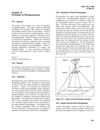
10-4. Geometry of Aerial Photography
The geometry of a single vertical photograph is shown
in Figure 10-1. The photographic negative is shown for
completeness, but in practice it is typical to work with
the photographic positive printed on paper, film, or
glass. The front nodal point of the camera lens is de-
fined as the exposure station of the photograph. The
nodal points are those points in the camera lens system
such that any light ray entering the lens and passing
through the front nodal point will emerge from the rear
nodal point travelling parallel to the incident light ray.
Therefore, the positive photograph can be shown on the
object side of the camera lens, positioned such that the
object point, the image point, and the exposure station
all lie on the same straight line. The line through the
lens nodal points and perpendicular to the image plane
intersects the image plane at the principal point. The
distance measured from the rear nodal point to the nega-
tive principal point or from the front nodal point to the
positive principal point is equal to the focal length f of
the camera lens.
10-5. Single Vertical Aerial Photography
Figure 10-1. Single vertical photograph geometry
Vertical photographs, exposed with the optical axis
vertical or as nearly vertical as possible, are the princi-
pal kind of photographs used for mapping. If the axis is
10-1

2. EM 1110-1-1000
31 Mar 93
perfectly vertical, the resulting photograph is termed a
"truly vertical" photograph. In spite of the precautions
taken to maintain the vertical camera axis, small tilts are
invariably present; but these tilts are usually less than
1 degree and they rarely exceed 3 degrees. Photographs
containing these small, unintentional tilts are called
"near vertical" or "tilted" photographs. Many of the
equations developed in this chapter are for truly vertical
photographs, but for certain work, they may be applied
to near vertical photos without serious error. Photo-
grammetric principles and practices have been
developed to account for tilted photographs, and no
accuracy whatsoever need be lost in using tilted
photographs.
a. Photographic scale. The scale of an aerial pho-
tograph can be defined as the ratio between an image
distance on the photograph and the corresponding hori-
zontal ground distance. Note that if a correct photo-
graphic scale ratio is to be computed using this defini-
tion, the image distance and the ground distance must be
measured in parallel horizontal planes. This condition
rarely occurs in practice since the photograph is likely
to be tilted and the ground surface is seldom a flat hori-
zontal plane. Therefore, scale will vary throughout the
format of a photograph, and photographic scale can be
defined only at a point.
(1) The scale at a point on a truly vertical photo-
graph is given by
(10-1)S
f
H h
where
S = photographic scale at a point
f = camera focal length
H= flying height above datum
h = elevation above datum of the point
Equation 10-1 is exact for truly vertical photographs and
is typically used to calculate scale on nearly vertical
photographs.
(2) In some instances, such as flight planning calcu-
lations, approximate scaled distances are adequate. If
all ground points are assumed to lie at an average eleva-
tion, an average photographic scale can be adopted for
direct measurements of ground distances. Average scale
is calculated by
(10-2)Save
f
H have
where have is the average ground elevation in the photo.
Then referring to the vertical photograph shown in Fig-
ure 10-2, the approximate horizontal length of the line
AB is
(10-3)D ≅
d H have
f
where
D = horizontal ground distance
d = photograph image distance
Figure 10-2. Horizontal ground coordinates from
single vertical photograph
10-2

3. EM 1110-1-1000
31 Mar 93
The flat terrain assumption, however, introduces scale
variation errors. For accurate determinations of horizon-
tal distances and angles, the scale variation caused by
elevation differences between points must be accounted
for in the photogrammetric solution.
b. Horizontal ground coordinates. Horizontal
ground distances and angles can be computed using
coordinate geometry if the horizontal coordinates of the
ground points are known. Figure 10-2 illustrates the
photogrammetric solution to determine horizontal
ground coordinates.
(1) Horizontal ground coordinates can be calculated
by dividing each photocoordinate by the true photo-
graphic scale at the image point. In equation form, the
horizontal ground coordinates of any point are given by
(10-4)
Xp
xp
(H hp
)
f
Yp
yp
(H hp
)
f
where
Xp,Yp = ground coordinates of point p
xp,yp = photocoordinates of point p
hp = ground elevation of point p
Note that these equations use a coordinate system de-
fined by the photocoordinate axes having an origin at
the photo principal point and the x-axis typically
through the midside fiducial in the direction of flight.
Then the local ground coordinate axes are placed paral-
lel to the photocoordinate axes with an origin at the
ground principal point.
(2) The equations for horizontal ground coordinates
are exact for truly vertical photographs and typically
used for near vertical photographs.
(3) After the horizontal ground coordinates of points
A and B in Figure 10-2 are computed, the horizontal
distance is given by
(10-5)DAB
(Xa
Xb
)2
(Ya
Yb
)2
This solution is not an approximation because the effect
of scale variation caused by unequal elevations is in-
cluded in the computation of the ground coordinates. It
is important to note, however, that the elevations ha and
hb must be known before the horizontal ground coordi-
nates can be computed. The need to know elevation can
be overcome if a stereo solution is used.
c. Relief displacement. Relief displacement is an-
other characteristic of the perspective geometry recorded
by an aerial photograph. The displacement of an image
point caused by changes in ground elevation is closely
related to photographic scale variation. Relief displace-
ment is evaluated when analyzing or planning mosaic or
orthophoto projects. Relief displacement is also a tool
that can be used in photo interpretation to determine
heights of vertical objects.
(1) The displacement of photographic images caused
by differences in elevation is illustrated in Figure 10-3.
The image displacement is always along radial lines
from the principal point of a truly vertical photograph or
the nadir of a tilted photograph. The magnitude of
relief displacement is given by the formula
(10-6)d
rh
H
where
d = image displacement
r = radial distance from the principal point to the
image point
H = flying height above ground
(2) Since the image displacement of a vertical object
can be measured on the photograph, Equation 10-6 can
be solved for the height of the object to obtain
(10-7)ht
d(H hbase
)
rtop
where
ht = vertical height of the object
hbase = elevation at the object base above datum
10-3

4. EM 1110-1-1000
31 Mar 93
Remember, heights of vertical objects can be determined
Figure 10-3. Relief displacement on a vertical
photograph
on a single photograph, but elevation above datum
cannot be determined.
10-6. Exterior Orientation of Tilted Photographs
Unavoidable aircraft tilts cause aerial photographs to be
exposed with the camera axis tilted slightly from verti-
cal, and the resulting pictures are called tilted photo-
graphs. The equations given above are exact for truly
vertical photographs, and they are used with near verti-
cal photography for planning, estimating, and photo
interpretation. However, an accurate photogrammetric
solution using aerial photographs must account for the
camera position and tilt at the instant of exposure.
a. The exterior orientation of a photograph is its
spatial position and angular orientation with respect to
the ground coordinate system. Six independent
parameters are required to define exterior orientation.
The space position is normally given by three-
dimensional coordinates of the exposure station in a
ground coordinate system. The vertical coordinate
corresponds to the flying height above datum. Angular
orientation is the amount and direction of tilt in the
photo. Three angles are sufficient to define angular
orientation, and two different systems are commonly
used: the tilt-swing-azimuth system (t-s-α) and the
omega-phi-kappa system (ω, φ, κ). The omega-phi-
kappa system possesses certain computational
advantages over the tilt-swing-azimuth system, but the
tilt-swing-azimuth system is perhaps more easily under-
stood. Figure 10-4 illustrates the parameters used to
express exterior orientation of an aerial photograph.
b. The tilt-swing-azimuth system is appropriate for
Figure 10-4. Exterior orientation of an aerial
photograph
hand calculations. An auxiliary photocoordinate system
is defined with an origin at the photo nadir and y′ axis
along the direction of tilt. The expression for scale on a
tilted photograph is
(10-8)
S
f
cos t
(y′ sin t)
H h
10-4

5. EM 1110-1-1000
31 Mar 93
where
y′ = auxiliary photocoordinate
t = photo tilt angle
c. The tilt of aerial mapping photography is seldom
large enough to require using tilted photograph equa-
tions for hand calculations when planning and estimat-
ing projects. However, Equation 10-8 does show that
scale is a function of tilt, and scale variation occurs on a
tilted photo even over flat terrain.
d. Since the swing angle s of a truly vertical photo-
graph is undefined, the omega-phi-kappa angular orien-
tation system is preferred when expressing exterior
orientation of any photograph. In the omega-phi-kappa
system, the angular orientation of a tilted photograph is
given in terms of three sequential rotation angles,
omega, phi, and kappa. These angles, shown also in
Figure 10-4, uniquely define the angular relationships
between the three image coordinate system axes of a
tilted photo and the three axes of the ground coordinate
system. Omega is a rotation about the x photographic
axis, phi is about the y-axis, and kappa is about the
z-axis.
e. The angular orientation of a truly vertical photo-
graph taken with the flight line in the ground X or east
direction is
ω = 0
φ = 0
κ = 0
The omega-phi-kappa angular orientation system is used
in analogic and analytical solutions to express the
exterior orientation of a photograph and produce
accurate map information from aerial photographs.
10-7. Stereoscopic Vision
Stereoscopic vision determines the distance to an object
by intersecting two lines of sight. In the human vision
system, the brain senses the parallactic angle between
the converging lines of sight and unconsciously associ-
ates the angle with a distance. Overlapping aerial pho-
tographs can be viewed stereoscopically with the aid of
a stereoscope. The stereoscope forces the left eye to
view the left photograph and the right eye to view the
right photograph. Since the right photograph images the
same terrain as the left photograph, but from a different
exposure station, the brain perceives a parallactic angle
when the two images are fused into one. As the viewer
scans the entire overlap area of the two photographs, a
continuous stereomodel of the ground surface can be
seen. The stereomodel can be measured in three dimen-
sions, yielding the elevation and horizontal position of
unknown points. The limitation that elevation cannot be
determined in a single photograph solution is overcome
by the use of stereophotography.
a. Lens stereoscope. A lens or pocket stereoscope is
a low-cost instrument that is very useful in the field as
well as the office. It offers a fixed magnification, typi-
cally 2.5X. The lens stereoscope is useful for photo
interpretation, control point design, and verification of
mapped planimetric and topographic features.
b. Mirror stereoscope. A mirror stereoscope can be
used for the same functions as a lens, but is not appro-
priate for field use. The mirror stereoscope has a wider
field of view at the nominal magnification ratio. Since
photographs can be held fixed for stereo viewing under
a mirror stereoscope, the instrument is useful for simple
stereoscopic measurements. Mirror stereoscopes can be
equipped with binocular eyepieces that yield 6X and 9X
magnification. The high magnification helps to identify,
interpret, and measure photographed features.
c. Floating mark. Stereoscopic measurements are
possible if a floating mark is introduced in the viewing
system. Identical halfmarks, such as a small filled circle
or a small cross, are put in the field of view of each
eye. As the stereomodel surface is viewed, the two
halfmarks are viewed against the photographed scene by
each eye. If the halfmark positions are properly
adjusted, the brain will fuse their images into a single
floating mark that appears in three-dimensional space
relative to the stereomodel. By moving the halfmarks
parallel to the viewer’s eye base, the floating mark can
be adjusted until it is perceived to lie on the stereo-
model surface. At this point, the two halfmarks are on
the identical or conjugate image points of two different
photographs. The horizontal position and elevation of
the mark can be determined and plotted on a map. The
importance of the floating mark is that all points in a
stereomodel can be measured and mapped. Thus, indis-
tinct points, such as hilltops, centers of road intersec-
tions, and contours can be mapped in three dimensions
from the stereomodel.
10-5

6. EM 1110-1-1000
31 Mar 93
10-8. Geometry of Aerial Stereophotographs
The basic unit of photogrammetric mapping is the stere-
omodel formed in the overlapping ground coverage of
successive photographs along a flight line. Figure 10-5
illustrates the ground coverage along three contiguous
flight lines in a block of aerial photographs. Along each
flight line, the overlap of photographs, termed end lap,
is typically designed to be 60 percent. End lap must be
at least 55 percent to ensure continuous stereoscopic
coverage and provide a minimum triple overlap area
where stereomodels can be matched together. Between
adjacent flight lines, the overlap of strips, termed side
lap, is typically designed to be 30 percent. Side lap
must be at least 20 percent to ensure continuous stereo-
scopic coverage.
a. Stereomodel dimensions. For project planning
Figure 10-5. Aerial photography stereomodel and
neat model
and estimating, photograph and stereomodel ground
dimensions are computed by assuming truly vertical
photography and flat terrain at average ground elevation.
(1) Using average photographic scale, the ground
coverage G of one side of a square format photograph is
(10-9)G
d
Save
where d is the negative format dimension. The flying
height above datum is also found using average scale
and average ground elevation.
(10-10)H have
f
Save
(2) Let B represent the air base between exposures
in the strip. Then from the required photo end lap Elap
(10-11)
B G








1
Elap
100
(3) Let W represent the distance between adjacent
flight lines. Then from the required side lap Slap
(10-12)
W G








1
Slap
100
(4) Match lines between contiguous stereomodels
pass through the center of the triple overlap area and the
center of the side lap area. These match lines bound the
neat model area, the net area to be mapped within each
stereomodel. The neat model has width equal to B and
length equal to W.
b. Parallax equations. The parallax equations may
be used for simple stereo analysis of vertical aerial
photographs taken from equal flying heights—that is,
the camera axes are parallel to one another and perpen-
dicular to the air base. Conjugate image points in the
overlap area of two truly vertical aerial photographs
may be projected as shown in Figure 10-6. When the
photographs are properly oriented with respect to one
another, the conjugate image rays recorded by the
camera will intersect at the true spatial location of the
object point. Images of an object point A appear on the
left and right photos at a and a′, respectively. The
planimetric position of point A on the ground is given in
terms of ground coordinates XA and YA. The XY
ground axis system has its origin at the datum principal
point O of the left photograph; the X-axis is in the same
vertical plane as the photographic x and x′ flight axes;
and the Y-axis passes through the datum principal point
of the left photograph and is perpendicular to the
X-axis.
10-6

7. EM 1110-1-1000
31 Mar 93
(1) Photographic parallax is defined as the apparent
movement of the image point across the image plane of
the camera as the camera exposure station moves along
the flight line. The parallax of the image point in
Figure 10-6 is
Figure 10-6. Stereopair of vertical aerial photographs
(10-13)Pa
xa
xa
′
where xa and xa′ are coordinate distances on the left and
right photographs, respectively. Since parallactic image
motion is parallel to the movement of the camera, the
parallax coordinate system must be parallel to the direc-
tion of flight. All parallax occurs along the x-axis in
the axis of flight photocoordinate system. The y and y′
coordinates are equal.
(2) Given truly vertical aerial photographs and
photocoordinates measured in the axis of flight system,
the following parallax equations can be derived:
(10-14)
X
xB
p
Y
yB
p
h H
fB
p
where
X,Y = horizontal ground coordinates
x,y = photocoordinates on the left photograph
p = parallax
Note that the origin of the ground coordinate system is
at the ground principal point of the left photograph, and
the X-axis is parallel to the flight line.
c. Parallax difference equation. The parallax equa-
tions given in b above assume that the photographs are
truly vertical and exposed from equal flying heights;
thus, the camera axes are parallel to one another and
perpendicular to the air base. Scale variation and relief
displacement are not regarded as errors in the parallax
method since these effects are measured as image paral-
lax and used to compute elevations; however, tilted
photographs, unequal flying heights, and image distor-
tions seriously affect the accuracy of the parallax
method. Absolute elevations are difficult to determine
using the parallax equations given in b above because
small errors in parallax will cause large errors in the
vertical distance H-h. More precise results are obtained
if differences in elevation are determined using the
parallax difference formula
(10-15)hA
hC
∆p(H hC
)
Pa
where
hA = elevation of point A above datum
hC = elevation of point C above datum
10-7

8. EM 1110-1-1000
31 Mar 93
Pa = parallax of image point a
Pc = parallax of image point c
∆p = difference in parallax (Pc - Pa)
The formula should be applied to points that are close to
one another on the photo format. The differencing
technique cancels out the systematic errors affecting the
parallax of each point. If C is a vertical control point,
the absolute elevation of A can be determined by this
method.
10-9. Fundamental Photogrammetric Problems
The fundamental photogrammetric problems are resec-
tion and intersection. All photogrammetric procedures
are composed of these two basic problems.
a. Resection. Resection is the process of recovering
the exterior orientation of a single photograph from
image measurements of ground control points. In a
spatial resection, the image rays from total ground
control points (horizontal position and elevation known)
are made to resect through the lens nodal point (expo-
sure station) to their image position on the photograph.
The resection process forces the photograph to the same
spatial position and angular orientation it had when the
exposure was taken. The solution requires at least three
total control points that do not lie in a straight line, and
the interior orientation parameters, focal length, and
principal point location. In aerial photogrammetric
mapping, the exact camera position and orientation are
generally unknown. The exterior orientation must be
determined from known ground control points by the
resection principle.
b. Intersection. Intersection is the process of photo-
grammetrically determining the spatial position of
ground points by intersecting image rays from two or
more photographs. If the interior and exterior orienta-
tion parameters of the photographs are known, then
conjugate image rays can be projected from the photo-
graph through the lens nodal point (exposure station) to
the ground space. Two or more image rays intersecting
at a common point will determine the horizontal posi-
tion and elevation of the point. Map positions of points
are determined by the intersection principle from cor-
rectly oriented photographs.
10-10. Photogrammetric Solution Methods
Correct and accurate photogrammetric solutions must
include all interior and exterior orientation parameters.
Each orientation parameter must be modeled if the re-
corded image ray is to be correctly projected and an
accurate photogrammetric product obtained. Interior
orientation parameters include the camera focal length
and the position of the photo principal point. Typically
the interior orientation is known from camera calibra-
tion. Exterior orientation parameters include the camera
position coordinates and the three orientation angles.
Typically, the exterior orientation is determined by
resection principles as part of the photogrammetric
solution. The remaining parameters are the ground
coordinates of the point to be mapped. Planimetric and
topographic details are mapped by intersecting conjugate
image rays from two correctly oriented photographs.
Methods of solving the fundamental photogrammetric
problems may be classified as analog or analytical
solutions.
a. Analog solutions. Analog photogrammetric solu-
tions use optical or mechanical instruments to form a
scale model of the image rays recorded by the camera.
An optical analog instrument projects a transparency of
the image through a lens such that the camera bundle of
image rays is accurately reproduced and the projected
image is brought to focus at some finite distance from
the lens. A mechanical analog instrument uses a
straight metal rod, a space rod, to represent the image
ray from the image point, through the lens perspective
center, to the modelled ground point. Analog instru-
ments are limited in function (focal length, model scale
enlargement, flight geometry) by the physical constraints
of the analog mechanism. They are limited in accuracy
by the calibration of the analog mechanism and by un-
modelled systematic errors. Analog instruments cannot
effectively compensate for differential or nonlinear
image and film deformation errors.
b. Analytical solutions. An analytical photogram-
metric solution uses a mathematical model to represent
the image rays recorded by the camera. The image ray
is assumed to be a straight line through the image point,
the exposure station, and the ground point. The follow-
ing collinearity equation expresses this condition:
10-8

9. EM 1110-1-1000
31 Mar 93
(10-16)
where
x,y = measured photocoordinates
xo,yo = principal point photocoordinates
mij = nine direction cosines expressing the
angular orientation
X,Y,Z = ground point coordinates
XL,YL,ZL = exposure station coordinates
The collinearity condition equations include all interior
and exterior orientation parameters required to solve the
resection and intersection problems accurately. Analyti-
cal solutions consist of systems of collinearity equations
relating measured image photocoordinates to known and
unknown parameters or the photogrammetric problem.
The equations are solved simultaneously to determine
the unknown parameters. However, since there are
usually redundant measurements producing more equa-
tions than there are unknowns in the problem, a least
squares adjustment is used to estimate the unknown
parameters. The least squares adjustment algorithm
includes residuals vx and vy on the measured photocoor-
dinates that estimate random measurement error.
10-11. Terrestrial Photogrammetry
a. Definition. Terrestrial photogrammetry refers to
applications where the camera is supported on the sur-
face of the earth. Typically the camera is mounted on a
tripod and the camera axis is oriented in or near the
horizontal plane. When the distance to the object is less
than approximately 300 m, the method is often referred
to as close-range photogrammetry.
b. Applications. Terrestrial photogrammetry tech-
niques can be applied to measuring and mapping large
vertical surfaces. These applications include topo-
graphic mapping of rugged terrain and vertical cliffs,
deformation measurement of structures, and architectural
mapping of buildings. Close-range applications include
measuring and calibrating irregular surfaces such as
antenna reflectors and industrial assembly jigs, and
three-dimensional mapping of industrial installations and
construction sites.
c. Instrumentation
(1) Cameras. Cameras for engineering applications
of terrestrial photogrammetry should be stable,
calibrated metric cameras similar to aerial cameras. For
highest accuracy, some cameras expose the image
directly on glass planes to ensure image plane flatness.
Film type cameras should have a film-flattening device.
Terrestrial cameras are available in a range of focal
lengths and format size. If the camera is combined with
angle measuring capability for orienting the camera axis
in a known direction, the instrument is referred to as a
phototheodolite. Stereometric cameras are two cameras
rigidly fixed to a base bar. Since the base is usually
short, stereometric cameras fall into the close-range
category.
(2) Stereoplotters. Some specialized stereoplotters
have been developed specifically for terrestrial applica-
tions; however, these instruments are not typically
available in the United States photogrammetric industry.
Some analog stereoplotters can accommodate some
terrestrial and close-range cameras; but often incompati-
ble focal lengths, format sizes, and depth of field con-
straints make analog stereoplotters unusable for this
work. Analytical stereoplotters can accommodate terres-
trial and close-range cameras because no mechanical
constraints are placed on the mathematical projection.
Of course, monocomparators and analytical software
work equally well for precise applications of point
mapping.
d. Methods. The photogrammetric principles dis-
cussed in this chapter apply also to the terrestrial solu-
tions. Terrestrial photogrammetry differs from aerial
photogrammetry in the fact that the camera is acces-
sible. Thus, the camera position and orientation can be
measured. Theoretically this eliminates the need for
control points and resection to orient the camera. When
considering a terrestrial or close-range application, addi-
tional consideration must be given to optimum camera
location geometry, focusing requirements of the camera,
and depth of field requirements to capture the object to
be measured.
10-9

10. EM 1110-1-1000
31 Mar 93
Section II
Stereoscopic Plotting Instruments
10-12. General
A general overview of existing stereoplotter designs and
general operating procedures is presented in this chapter.
For the purposes of this chapter, only instruments that
perform a complete restitution of the interior and
exterior orientation of the photography taken will be
considered. Although all types of stereoplotters are
discussed, it is expected that analytical stereoplotters
will become the industry standard because of accuracy,
efficiency, and capability.
10-13. Types of Stereoplotters
The three main component systems in all stereoplotters
are the projection system, the viewing system, and the
measuring and tracing system. Stereoplotters are most
often grouped according to the type of projection system
used in the instrument.
a. Direct-optical projection stereoplotters. Direct-
optical projection stereoplotters project a transparent
positive of the original negative optically through a lens
to recreate the bundle of image rays recorded by the
cameras. This type of stereoplotter was the precursor of
modern mechanical projection and analytical stereoplot-
ters. Briefly, these stereoplotters use a fixed focal
length lens for projection so that the principal distance
and the projection distance of the instrument are fixed.
Thus, the enlargement ratio from positive to stereomodel
is also fixed. For a typical "Kelsh-type" instrument, the
enlargement ratio of the stereomodel is five times the
contact positive scale. The stereomodel is viewed
directly on a reflecting platen in the model space. The
floating mark is on the platen, and as the mark is moved
through the model, its position is traced directly onto a
map manuscript below the mark. The vertical move-
ment of the platen is read out at model scale as the
elevation of the floating mark. Direct-optical projection
stereoplotters are classified as the least accurate instru-
ment type. They have been replaced in practice by
mechanical projection and analytical stereoplotters.
b. Mechanical projection stereoplotters. Mechani-
cal projection stereoplotters are analog instruments that
recreate the image ray using a metal space rod. The
space rod pivots in a fixed gimbal joint representing the
lens nodal point. Two space rods from adjacent diapos-
itives intersect in the model space to define the terrain
point. Since no lens is included in the projection
system, the principal distance and projection distance
along the space rod can be varied. Usually a small
range of camera focal lengths can be accommodated,
and model scale can be varied within the mechanical
limits of the instrument.
(1) The viewing system of a mechanical projection
stereoplotter is an optical train system of lenses and
prisms similar in principle to a mirror stereoscope. The
operator perceives the stereomodel by looking directly at
the positive image. Image magnification is included to
increase the precision of the floating mark placement in
the stereomodel.
(2) The floating mark is included in the optical train.
Its position in the model space corresponds to the inter-
section of the space rods representing the two conjugate
image rays. The model carriage where the space rods
intersect may be free moving. The model carriage may
include a pencil mount, and the carriage is hand-driven
to trace out a map manuscript. The model carriage may
be connected to a mechanical drive that can be digitally
encoded. Thus, the movement of the floating mark is
converted to digital x-y-z model coordinates in three
dimensions.
(3) The accuracy of mechanical projection stereo-
plotters will typically be in the medium to high range.
Plotters designed for map compilation are in the medi-
um range. These plotters typically have free-moving
model carriages that are hand-driven during map compi-
lation. The Kern PG2, Galileo G6, and Wild B8 are
some examples of medium-accuracy mechanical projec-
tion stereoplotters used for map compilation. Mechani-
cal projection stereoplotters in the high-accuracy range
warrant more precise measurement of the stereomodel
space. In these instruments, the model carriage is
mechanically driven and controlled by operator hand
wheels and foot disk or similar control devices. These
stereoplotters are also more massive and stable instru-
ments than the medium-accuracy compilation instru-
ments, and typically they are universal instruments
capable of analog aerotriangulation. The Wild A8,
Zeiss C8, and Jena Stereometrograph are some examples
of these instrument types.
c. Analytical stereoplotters. Analytical stereoplotters
use a mathematical image ray projection based on the
collinearity equation model. The mechanical component
of the instrument consists of a precise computer-
controlled stereocomparator. Since the photo stages
must move only in the x and y image directions, the
measurement system can be built to produce a highly
10-10

11. EM 1110-1-1000
31 Mar 93
accurate and precise image measurement. The x and y
photocoordinates are encoded, and all interior and
exterior orientation parameters are included in the
mathematical projection model. Except for the positive
format size that will fit on the photo stage, the analytical
stereoplotter has no physical constraints on the camera
focal length or model scale that can be accommodated.
(1) The viewing system is an optical train system
typically equipped with zoom optics. The measuring
mark included in the viewing system may be changeable
in style, size, and color. The illumination system should
have an adjustable intensity for each eye.
(2) The measuring system consists of an input
device for the operator to move the model point in three
dimensions. The input device is encoded, and the digi-
tal measure of the model point movement is sent to the
computer. The software then drives the stages to the
proper location accounting for interior and exterior
orientation parameters. These operations occur in real
time so that the operator, looking in the eyepieces, sees
the fused image of the floating mark moving in three
dimensions relative to the stereomodel surface. The
operator’s input device for model position may be a
hand-driven free-moving digitizer cursor on instruments
designed primarily for compilation, or it may be a hand
wheel/foot disk control or similar device on instruments
supporting fine pointing for aerotriangulation.
(3) Analytical stereoplotters are more accurate than
analogic stereoplotters because the interior orientation
parameters of the camera are included in the projection
software. Therefore, any systematic error in the photo-
graphy can be corrected in the photocoordinates before
the photogrammetric projection is performed. Correct-
ing for differential film deformations, lens distortions,
and atmospheric refraction justifies measuring the photo-
coordinates to accuracies of 0.003 mm and smaller in
analytical stereoplotters. To achieve this accuracy, the
analytical stereoplotter must have the capability to per-
form a stage calibration using measurements of refer-
ence grid lines etched on the photo stage.
(4) Analytical stereoplotters capable of precise map
compilation and aerotriangulation measurements include
(but are not limited to) the Zeiss Planicomp P series, the
Wild (now Leica) AC and BC series, the Kern (now
Leica) DSR series, the Intergraph Intermap, and the
Galileo Digicart (Figure 7-5).
d. Digital stereoplotters. The next generation of
stereoplotters will be digital (or soft copy) stereoplotters.
These instruments will display a digital image on a
workstation screen in place of a film or glass diaposi-
tive. The instrument will operate as an analytical
stereoplotter except that the digital image will be viewed
and measured. The accuracy of digital stereoplotters is
governed by the pixel size of the digital image. The
pixel size directly influences the resolution of the photo-
coordinate measurement. A digital stereoplotter can be
classified according to the photocoordinate observation
error at image scale. Then it should be comparable to
an analog or analytical stereoplotter having the same
observation error, and the standards and guidelines in
this manual should be equally as applicable. See also
paragraph 10-15.
10-14. Stereoplotter Operations
All stereoplotters, whether analog or analytical, must
be set up for measuring or mapping in three
consecutive steps: interior orientation, relative orien-
tation, and absolute orientation.
a. Interior orientation. Interior orientation in-
volves placing the photographs in proper relation to
the perspective center of the stereoplotter by match-
ing the fiducial marks to corresponding marks on the
photography holders and by setting the principal
distances of the stereoplotter to correspond to the
focal length of the camera (adjusted for overall film
shrinkage).
b. Relative orientation. Relative orientation in-
volves reproducing in the stereoplotter the relative
angular relationship that existed between the camera
orientations in space when the photographs were
taken. This is an iterative process and should result
in a stereoscopic model easily viewed, in every part,
without "y parallax"—the separation of the two
images so they do not fuse into a stereoscopic model.
When this step is complete, there exists in the stereo-
plotter a stereoscopic model for which three-
dimensional coordinates may be measured at any
point; but it may not be exactly the desired scale, and
it may not be level—water surfaces may be tipped.
c. Absolute orientation. Absolute orientation uses
the known ground coordinates of points identifiable
in the stereoscopic model to scale and to level the
model. When this step is completed, the X, Y, and Z
ground coordinates of any point on the stereoscopic
model may be measured and/or mapped.
10-11

12. EM 1110-1-1000
31 Mar 93
10-15. Stereoplotter Accuracies
Stereoplotter accuracies are best expressed in terms of
observation error at diapositive scale. In this way,
instruments can be compared based on the fundamental
measurement of image position on the positive. Mea-
surement error on the positive can be projected to the
model space so that expected horizontal and vertical
error in the map compilation can be estimated. Stereo-
plotter accuracy affects the maximum allowable
enlargement from photo scale to map scale and the
minimum CI that can be plotted from given photo scale.
The enlargement ratio and the empirical C-factor are
discussed in Chapter 7, and maximum values for these
two factors are specified in Chapter 2.
10-16. Stereoplotter Output Devices
Stereoplotters are connected to a variety of devices for
plotting or recording line work and digital data.
Although the direct tracing of map manuscripts on a
stereoplotter is a form of output, it is expected that
modern stereoplotters will be encoded and interfaced to
a graphical or digital output device. Examples of these
output devices are shown in Chapter 7.
a. Stereoplotters may be computer assisted. The
movement of the measuring mark of these stereoplotters
is digitally encoded. The digital signal is sent directly
to a computer-controlled coordinatograph. The operator
can include feature codes in the digital signal that the
computer can interpret to connect points with the proper
line weight and type, plot symbols at point locations,
label features with text, etc. The final map product can
be produced at the manuscript stage by an experienced
operator.
b. A digitally encoded stereoplotter may also be
interfaced to a digital compilation software system in
which the compiled line work and annotations appear on
a workstation screen. Similar to the computer-assisted
stereoplotter and coordinatograph, the compilation on
the workstation screen can be displayed with proper line
weights (or colors and layers), line types, symbols, and
feature labels. In addition, since the map exists in a
digital computer file, basic map editing can be done as
the manuscript progresses. Typically, the digital compi-
lation file is converted (or translated) to a full CADD
design file where it can be merged with adjacent
compiled stereomodels and final map editing performed.
The deliverable product from these systems is often in
digital form on computer tape or disk.
Section III
Ground Control Datums and Coordinate
Reference Systems
10-17. General
Photogrammetric ground control consists of any points
whose positions are known in a ground reference coor-
dinate system, and whose images can be positively
identified in the photographs. Ground control provides
the means for orienting or relating aerial photographs
and stereomodels to the ground. Almost every phase of
photogrammetric work requires some ground control.
Photogrammetric control is generally classified as either
horizontal control (the position of the point is known
with respect to a horizontal datum), or vertical control
(the elevation of the point is known with respect to a
vertical datum). Sometimes both horizontal and vertical
object space positions of points are known so that these
points serve a dual control purpose. Such points may
be referred to as total control.
10-18. Coordinate Datums and Reference
Systems
A datum is a reference surface on which a coordinate
system is defined. In surveying and mapping, many
datums and many coordinate systems can be defined
that will express the position of points on the earth’s
surface. It is of utmost importance to know the
coordinate system used to reference any control survey
or map. Control survey or map data sets referenced to
different coordinate systems cannot be combined unless
a transformation of one coordinate system into the other
is performed. A detailed discussion of coordinate
datums and transformations is given by Soler and
Hothem (1988, 1989).
a. Horizontal geodetic datum. Datums are often
separated into horizontal and vertical datums. A hori-
zontal geodetic datum uses an ellipsoid as the reference
surface. The size and shape of the ellipsoid are chosen
to give the best fit to the earth on a global basis or on a
regional or continental basis. Many different ellipsoids
have been proposed. The datum definition is completed
by orienting a specific ellipsoid to the earth and defining
a coordinate system.
(1) Curvilinear coordinates. Geodetic longitude and
latitude are curvilinear coordinates that define the posi-
tion of a point on the curved ellipsoid surface. The
coordinates are expressed in angular units. (Longitude
10-12

13. EM 1110-1-1000
31 Mar 93
is the angle measured in the plane of the equator from
the reference meridian through Greenwich, England, to
the meridian through the point. Latitude is the angle in
the plane of the meridian through the point from the
equator to the normal through the point.) A geodetic
height can also be defined as the distance along the
normal from the surface of the ellipsoid to the point.
(2) Geocentric coordinates. Geocentric coordinates
are defined for a given datum by placing the origin of a
right-handed spatial rectangular coordinate system at the
center of the reference ellipsoid. The z-axis coincides
with the semiminor axis of the ellipsoid. The x- and y-
axes are in the plane of the equator with the x-axis
through 0-degree longitude. Simple Cartesian coordi-
nate computations can be performed in the geocentric
system. The ellipsoid parameters and curved reference
surface are eliminated from the computations
(Figure 10-7).
(3) Local rectangular coordinates. A local rectan-
Figure 10-7. Coordinate reference systems
gular coordinate system can be defined for a given
project area. The geocentric coordinate axes are trans-
lated to a convenient point in or near the project area.
Then the x-y-z geocentric axes are rotated to align with
local east, north, and up (along the normal), respec-
tively, at the point. Local rectangular coordinates will
appear more natural with respect to the terrain, and the
coordinate magnitudes will be smaller for computations.
Photogrammetric aerotriangulation should be computed
in a local rectangular system (especially for large project
areas) since earth curvature and map projection distor-
tion are not present in Cartesian coordinates.
(4) North American Datum of 1927. In the United
States, two horizontal datums are commonly
encountered in engineering surveying and mapping: the
North American Datum of 1927 (NAD 27) and the
North American Datum of 1983 (NAD 83) (Table 10-3).
NAD 27, a datum defined by an adjustment begun in
1927 of the national control point network, is a conti-
nental datum referenced to the Clarke 1866 ellipsoid.
The ellipsoid is positioned and oriented to closely fit the
geoid throughout the North American continent. Since
the NAD 27 adjustment, new control surveys were
added to the network by holding the original framework
fixed and adjusting the new survey to fit the original.
As the network grew without readjustment, distortions
were found that demanded a readjustment of the net-
work to meet modern surveying requirements.
(5) North American Datum of 1983. NAD 83 is a
rigorous least squares adjustment of the entire national
control network incorporating modern high-precision
traverse and satellite measurements. NAD 83 is a
global datum referenced to the Geodetic Reference
System of 1980 ellipsoid. The ellipsoid is earth-
centered and designed to be a best fit to the global
geoid. Thus, the NAD 83 datum will have a larger
geoid-to-ellipsoid separation than the NAD 27 datum in
the United States. Since NAD 83 is a readjustment of
the original observations in the control network, it is not
possible to directly transform coordinates from one
datum to the other. Interpolation methods using control
points adjusted in both datums have been programmed
by the NGS for the purpose of estimating the NAD 83
coordinates of points surveyed in the NAD 27 datum.
Although the NAD 27 datum is still used, it should
gradually be replaced by the NAD 83 datum.
b. Vertical geodetic datum. A vertical geodetic
datum is a reference system for measuring vertical posi-
tion or elevation. The reference surface is the geoid,
which is an equipotential gravity surface that best
approximates mean sea level. Elevation above mean sea
level (the geoid) is measured along the direction of
gravity, perpendicular to the equipotential surfaces. In
the United States, the vertical geodetic datum is the
10-13

14. EM 1110-1-1000
31 Mar 93
Table 10-3
Comparison of NAD 27 and NAD 83 Datum Elements
Datum Element NAD 27 NAD 83
Reference Ellipse
Datum Point
Best Fitting
Adjustment
Clarke 1866
a = 6,378,206.4 m
b = 6,356,583.8 m
Meades Ranch Station
North America
Terrestrial data for 25,000 stations and
piecewise fits
GRS 80
a = 6,378,137 m
f = 1/298.2572221
Earth’s Mass Center
Global
Terrestrial and satellite data for 250,000+
stations
Note:
1. a = length of semimajor axis of ellipsoid.
b = length of semiminor axis of ellipsoid.
f = flattening of ellipsoid.
National Geodetic Vertical Datum of 1929. The eleva-
tion of a point can be combined with the horizontal
position on the ellipsoid to define a three-dimensional
coordinate, latitude, longitude, and height (φ, λ, h), by
the relationship
(10-17)h H N
where
h = height above the ellipsoid
H = elevation above the geoid
N = geoid separation above the ellipsoid
c. Map projections. A map projection is a mathe-
matical function that defines a relationship of coordi-
nates between the ellipsoid and a plane. The purpose of
a map projection is to display the curved earth surface
on a flat plane that can be printed on a sheet of paper.
If field survey observations are reduced to the plane, the
computation and adjustment of horizontal control posi-
tions can be carried out in two-dimensional Cartesian
coordinates. The need for more involved geodetic sur-
vey computations can be eliminated.
(1) The final map reference system is a plane
developed from a regular mathematical surface. Devel-
opable surfaces that can be rolled out into a plane in-
clude a plane, a cone, and a cylinder. The ideal map
projection would display all distances and directions
correctly, all areas would retain their correct shape and
relative size, meridians and parallels would intersect at
right angles, and great circles and rhumb lines would be
represented as straight lines. Obviously, the earth’s
surface, being spherical, cannot be developed upon a
plane without distortion of some of these quantities.
(2) In engineering surveying and mapping, correct
depiction of shapes is important. Thus, the charac-
teristic of conformality is enforced in projections used
for large-scale mapping. This is accomplished by math-
ematically constraining the projection scale factor at a
point, whatever it may be, such that it is the same in all
directions from that point. This characteristic of a pro-
jection preserves angles between infinitesimal lines.
That is, all lines on the grid cut each other at the same
angles as do the corresponding lines on the ellipsoid for
very short lines. Hence, for a small area, there is no
local distortion of shape. But since the scale must
change from point to point, distortion of shape can exist
over large areas. Remember that the distortion present
in any map projection is not an "error" since it is a
mathematically defined function. The distortion must
simply be accounted for in transforming data from map
to ground.
(3) The most commonly encountered map projec-
tions in engineering surveying and mapping are the
State Plane Coordinate Systems (SPCS). NGS has
developed SPCS’s for each state, and many states have
formally adopted the systems by legislative action. The
SPCS’s are based on the Lambert Conformal Conic
Projection or the transverse Mercator projection. For
complete discussion of the SPCS’s refer to Stem (1989).
10-14

15. EM 1110-1-1000
31 Mar 93
(4) State Plane Coordinate Systems are defined for
both the NAD 27 and NAD 83 datums. For the
NAD 27 SPCS definition, the unit of length is the
US Survey Foot. For the NAD 83 SPCS definition, the
unit of length is variable among the states. Care must
be exercised when using NAD 83 SPCS values in feet
since either the US Survey Foot or the International
Foot may be used in a specific state or locality. The
conversion factors are given in paragraph 2-10a.
(5) Another commonly used plane coordinate pro-
jection system is the UTM projection. Since this is the
standard military reference system, operational support
mapping work may need to be compiled using this
system. The UTM system uses a Mercator cylindrical
projection with the axis of the cylinder oriented
perpendicular to the earth’s polar axis. The UTM coor-
dinate zones are uniformly spaced around the equator at
6-degree intervals and extend north and south from the
equator. A useful reference for the UTM system and
other map projections is Snyder (1982).
Section IV
Principles of Aerotriangulation
10-19. General
The principles of aerotriangulation are reviewed in this
section. The basic procedures for sequential and simul-
taneous aerotriangulation adjustment methods are dis-
cussed as background for Chapter 6. Emphasis is
placed on fully analytical aerotriangulation procedures.
10-20. Aerotriangulation Principles
a. Definition. Aerotriangulation is the simultaneous
space resection and space intersection of image rays
recorded by an aerial mapping camera. The spatial
direction of each image ray is determined by projecting
the ray from the front nodal point of the camera lens
through the image on the positive photograph. Conju-
gate image rays projected from two or more overlapping
photographs intersect at the common ground points to
define the three-dimensional space coordinates of each
point. The entire assembly of image rays is fit to
known ground control points in an adjustment process.
Thus, when the adjustment is complete, ground coordi-
nates of unknown ground points are determined by the
intersection of adjusted image rays. Simultaneously
with the ground point intersections, the exterior orienta-
tion of each photograph is determined by image ray
resection through the camera.
b. Purpose. The purpose of aerotriangulation is to
extend horizontal and vertical control from relatively
few ground survey control points to each unknown
ground point included in the solution. The supplemental
control points are called pass points, and they are used
to control subsequent photogrammetric mapping.
c. Geometric principles. The aerotriangulation
geometry along a strip of photography is illustrated in
Figure 10-8. Photogrammetric control extension re-
quires that a group of photographs be oriented with
respect to one another in a continuous strip or block
configuration. The exterior orientation of any photo-
graph that does not contain ground control is determined
entirely by the orientation of the adjacent photographs.
In a given aerotriangulation configuration, each
photograph contributes to the exterior orientation of the
adjacent photographs through the pass points located in
the triple overlap areas. The term triple overlap refers
to the ground area shared by two adjacent stereomodels
along the strip. The triple overlap area is imaged on
three consecutive photographs. Thus, when end lap is
specified to be 60 percent, the alternate photographs will
overlap each other by 20 percent at average terrain
elevation.
d. Pass points. A pass point is an image point that
is shared by three consecutive photographs (two consec-
utive stereomodels) along a strip. As the pass point is
positioned by one stereomodel, it can be used as control
to orient the adjacent stereomodel. Thus, the point
"passes" control along the strip. Only three-ray points
in the triple overlap area serve this pass point function.
A two-ray point in the stereomodel is an intersection
point only and does not contribute to the aerotriangula-
tion function unless it is also a ground control point. A
pass point that is shared between two adjacent strips is
called a tie point.
10-21. Aerotriangulation Methods
Aerotriangulation methods can be characterized in
several ways:
a. Photogrammetric projection method (analogic or
analytical).
b. Strip or block formation and adjustment method
(sequential or simultaneous).
c. Basic unit of adjustment (strip, stereomodel, or
image rays).
10-15

16. EM 1110-1-1000
31 Mar 93
Modern instruments and adjustment methods dictate that
Figure 10-8. Aerotriangulation geometry
an analytical adjustment of stereomodels or image rays
be emphasized.
a. Semianalytical aerotriangulation. Semianalytical
methods use the stereomodel as the basic unit of the
aerotriangulation process. Stereomodels may be formed
by either analogical or analytical methods. After
interior and relative orientation of each stereopair of
photographs, stereomodel coordinates are measured in
an arbitrary coordinate system defined in the model
space. For aerotriangulation purposes, the spatial
coordinates of the two exposure stations and each pass
point in the stereomodel are required.
(1) Sequential strip formation. A strip unit is
formed sequentially from the stereomodels by joining
them at the exposure station and pass points shared by
the new stereomodel and the previous stereomodel
already in the strip coordinate system. Each stereo-
model added to the strip provides the necessary points
to bring the succeeding stereomodel into the strip unit.
The sequential nature of the strip formation procedure
allows systematic errors to accumulate as the strip unit
is assembled from the individual stereomodels. Resid-
ual systematic errors in the interior orientation, the rela-
tive orientation, and the measurement system are
propagated down the strip causing the horizontal and
vertical strip coordinate datums to bow and twist. Al-
though it is difficult to measure and completely remove
individual systematic errors in each stereomodel, the
total effect of all the errors acting on a strip unit is
readily apparent after initially leveling and scaling the
assembled strip unit. Discrepancies at the horizontal
and vertical control coordinates are calculated by taking
the coordinate differences between the known position
of each control point and its position in the assembled
strip unit.
(2) Strip adjustment. The sequential strip formation
causes the X, Y, and Z coordinate discrepancies at the
control points to form smooth error curves. The error
curves can be approximated by second- or third-order
polynomial functions. Corrections to the strip pass point
coordinates are derived by evaluating the polynomial
functions at the strip location of each pass point. The
corrections are applied to the original strip coordinates
to complete the strip adjustment process.
(a) The polynomial functions model the error propa-
gation in a single strip unit. Block configurations may
be adjusted by using separate polynomials for each strip.
The unique strip units in a block are joined together at
tie points in the overlap area between strips. The
10-16

17. EM 1110-1-1000
31 Mar 93
polynomial functions adjusting adjacent strips are
constrained to yield the same adjusted coordinates at
each tie point in the block.
(b) The polynomial adjustment of aerotriangulation
is an approximate method that is less accurate than the
simultaneous adjustment of stereomodels or photo-
graphs. The purpose of polynomial strip adjustment in
modern aerotriangulation systems is to perform a pre-
liminary adjustment of all the photogrammetric and
ground survey measurements. The sequential strip
formation and polynomial adjustment is an excellent
way to detect blunders in the data and provide initial
approximations for use in simultaneous adjustments.
b. Simultaneous adjustment of stereomodels. The
adjustment of independent stereomodels as individual
units is the logical extension of the strip unit adjustment
discussed in the previous paragraph. Sequentially
formed strip units are not used, but rather all
stereomodels in an entire strip or block are simultane-
ously transformed into the ground coordinate system.
Stereomodels without ground control points are carried
into the ground coordinate system by the pass points
and exposure stations shared with adjacent stereomodels.
The simultaneous adjustment of stereomodels can rival
the simultaneous adjustment of photographs if the indi-
vidual stereomodels are corrected for all systematic
deformations. However, the development of analytical
stereoplotters that measure precise photocoordinates
warrants that the more rigorous fully analytical
aerotriangulation be required for all large-scale and
high-accuracy mapping.
c. Fully analytical aerotriangulation. Fully analyti-
cal aerotriangulation is a simultaneous adjustment solu-
tion of collinearity equations representing all the image
rays in a strip or block of photography. The adjustment
is often referred to as the "bundle" method. Although
the basic unit of adjustment is actually the individual
image ray, the solution determines the exterior orienta-
tion parameters of the bundle of image rays recorded by
each photograph, and the adjusted ground coordinates of
each ground intersection point in the ground coordinate
system.
Section V
Map Substitutes — Mosaics, Photo Maps, and
Orthophotographs
10-22. General
Map substitute refers to those products where the com-
piled planimetric line map is replaced or augmented by
the aerial photographic images. Since the photographic
image will have scale variation caused by the perspec-
tive view of the camera, photo tilt, and unequal flying
heights, each product must be evaluated according to
how the scale variation problem is treated. Scale varia-
tion may be ignored, as in an index mosaic, and an
approximate map substitute is obtained; or the scale
variation can be compensated, as in an orthophoto pro-
cess, and a nearly true map substitute can be obtained.
10-23. Aerial Mosaics
Aerial mosaics are constructed from sets of individual
adjoining aerial photographs. Typically, the outer edge
of the photo coverage of each print is trimmed back to a
selected match line, and the photos assembled by care-
fully matching ground detail along the match line. A
photo index mosaic is a rough composite of a number of
individual photographs of a flight line or set of flight
lines overlaid one on top of the other without trimming
the photo prints. This composite may itself be photo-
graphed onto a single piece of film. Mosaic and index
assemblies form a continuous representation of the ter-
rain covered by the photography. Photo maps are maps
using a photograph (or mosaic) as the base to which
limited cartographic detail such as names, route num-
bers, etc., are added. Generally, a photo map is con-
structed from an orthophoto, or from several
orthophotos mosaicked together.
10-24. Uses of Mosaics
The increased need for presenting a pictorial view of the
earth’s surface has led to the aerial mosaic as a means
of showing a complete view of large areas. Because a
single photo is limited in area, groups of photos are
combined into mosaics to provide the aerial picture.
Mosaics are of principal use for presenting synoptic
views of a relatively large area, and as indexes of indi-
vidual photographs. The features are usually labeled or
"annotated" to facilitate the recognition of critical areas,
or overlays may be prepared to show planning develop-
ments or contemplated changes in an area. For
example, a mosaic can show the location of a proposed
highway. Using this technique, laypersons, and particu-
larly property owners adjacent to the proposed highway,
can visualize its effect on their holdings. Photo indexes
are used as a visual record of the photographs of a
project and as a reference of availability of photographs
over a particular area of terrain. Photo maps are
particularly useful for land use, land cover delineation,
land planning, zoning, tax maps, and preliminary engi-
neering design.
10-17

18. EM 1110-1-1000
31 Mar 93
10-25. Methods of Mosaic Construction
There are three principal construction methods for the
making of mosaics:
a. From paper prints. This is the simplest method.
The paper prints that are to be joined are laid one on
top of the other so that commonly imaged terrain is
matched. Then the paper prints are cut, along a feature
if possible, so that the edge joins will be as inconspicu-
ous as possible. The photographs are matched and
pasted to a base. As necessary, the photographs are
stretched to assure a good match of features across the
join line. The completed mosaic may be photographed
if a reduced scale mosaic, such as an index mosaic, is
desired.
b. From negatives or diapositives. This method is
called photomechanical mosaicking. The negatives to be
used for the construction are overlaid and stud regis-
tered. After the join lines are selected, a mask is made
that is opaque on one side of the join line and clear on
the other. A negative of the mask is made for the other
photo of the pair to be joined. These masks are also
stud registered. After all negatives and masks have
been stud registered, a piece of unexposed film is put
down (in the darkroom) over the studs and the first
photo negative and its corresponding mask are registered
and an exposure made. The mask permits only that
portion of the unexposed film under the negative to be
exposed. Successive portions of the film are exposed as
this process is repeated for each negative and mask until
the whole film is exposed as a single mosaic.
c. From digital imagery. Digital (or digitized)
imagery can be used to create a mosaic. This method
has been used most commonly with small-scale satellite
photographs. The method is very computer intensive.
Either by human or automated correlation, common
points on the two images to be joined are selected. The
computer can then match each pixel of the one image
with the corresponding pixel of the second image. A
join line is decided upon and the two images digitally
"sheared" along the join line. The two sheared images
are then brought together into a single file having a
common pixel coordinate system.
10-26. Types of Mosaics and Air Photo Plan
Maps
Mosaics or air photo plans may be uncontrolled, semi-
uncontrolled, or controlled. They may be constructed
from unrectified, rectified, or differentially rectified
photographs. A controlled mosaic or air photo plan is
prepared using photographs that have been rectified to
an equal scale, while an uncontrolled mosaic is prepared
by a "best fit" match of a series of individual
photographs.
10-27. Orthophotographs
Orthophotographs are photographs constructed from
vertical or near-vertical aerial photographs, such that the
effects of central perspective, relief displacement, and
tilt are (practically) removed. The resulting
orthophotograph is an orthographic project.
a. Orthophotomaps. Orthophoto maps are
orthophotographs with overlaid line map data. The
common line data overlays include grids, property lines,
political boundaries, geographic names, and other
selected cultural features.
b. Limitation of orthophotographs. The original
aerial negative from which the orthophotograph is made
is a central projection and, as such, displays relief dis-
placement and obscuration of features. For example, a
building will obscure the terrain that lies behind it. This
obscuration results in gaps of information that can be
gotten only from other sources of information, such as
field survey or separate photograph. Also, optical
orthorectifying devices have a finite width and length
slot width that can "rectify" only to an average elevation
within that slot. Thus, small objects, such as trees,
buildings, etc., are not rectified at all. Normally, only a
"smoothed" approximation to the actual terrain is recti-
fied. Digital rectifiers with spot diameters as small as 5
to 25 micrometers can, to a much greater degree, over-
come this latter shortcoming.
10-28. Uses of Orthophotographs
Orthophotos and orthophoto maps are widely used for
general planning purposes. The complete and accurate
display of all features in a project area is an ideal medi-
um for demonstrating terrain features to laypersons.
Proposed designs of engineering projects can be super-
imposed on the orthophoto map for a vivid understand-
ing of work to be accomplished. Many factors must be
considered before deciding on a photomap product in-
stead of a topographical map product. The intended use
of the product needs to be classified exactly, together
with the accuracy required and whether height informa-
tion is required or not. For many USACE engineering,
operations, and maintenance activities, rectified air
10-18

19. EM 1110-1-1000
31 Mar 93
photo plan sheets may be used in lieu of fully rectified
orthophotographs.
10-29. Methods of Orthophotograph
Preparation
Orthophotographs are prepared from pairs of overlap-
ping aerial photographs using specially designed ortho-
plotting instruments. The photographs are oriented in
the instrument in the conventional manner for standard
stereo photogrammetric mapping. The requirements for
ground control or control to be established by aerotrian-
gulation are the same as for photogrammetric mapping.
The instrument provides the means of scanning the
stereomodel to effect corrections for the varying scales
caused by topographic relief. The tilt and other
distortions are corrected in the orientation of the
stereomodel.
10-19