1. Bayesian Forecasting of Financial Time Series with
Stop-Loss Order
S. Dablemont (1)
, S. Van Bellegem (2)
, M. Verleysen (1)
Keywords
Finance, Forecasting, Stochastic, Bayesian Filters
1 Abstract
A Model of Trading forecasts the first stopping-time, the "High" and "Low" of an asset
over an interval of three hours, when this asset crosses for the first time a threshold selected
by the trader. To this end, we use high-frequency "tick-by-tick" data without resampling.
This Model of Trading is based on a Dynamic State Space Representation, using Stochastic
Bayes’ Filters for generalization.
2 Introduction
Based on martingales and stochastic integrals in the theory of continuous trading, and
on the market efficiency principle, it is often assumed that the best expectation of the
tomorrow price should be the today price, and looking at past data for an estimation of
the future is not useful, see (Harrison and Pliska, 1981), (Franke et al., 2002). But if this
assumption is wrong, the conclusion that forecasting is impossible is also questionable, see
(Olsen et al., 1992). Moreover practitioners use the technical analysis on past prices and
technicians are usually fond of detecting geometric patterns in price history to generate
trading decisions. Economists desire more systematic approaches so that such subjectivity
has been criticized. However some studies tried to overcome this inadequacy, see (Lo et
al., 2000).
The topic of this paper is the forecasting of the first stopping time, when prices cross for
the first time a "High" or "Low" threshold defined by the trader, estimated from a trading
model, and based on an empirical functional analysis, using a very high frequency data set,
as "tick-by-tick" asset prices, without resampling, and using a Stop-Loss Order to close
the position in case of bad prediction.
There is a distinction between a price forecasting and a trading recommendation. A trad-
ing model includes a price forecasting, but must also account for the specific constraints of
the trader because it is constrained by the trading history and the positions to which he is
committed. A trading model thus goes beyond a price forecasting so that it must decide
1
Université catholique de Louvain, École Polytechnique de Louvain, Machine Learning Group
3, Place du Levant, B-1348 Louvain-la-Neuve - BELGIUM, Tel : +32 10 47 25 51, E-mail : {dablemont,
verleysen}@dice.ucl.ac.be
2
Toulouse School of Economics GREMAQ
21, Allée de Brienne, F-31000 Toulouse - France, Tel : +33 56 11 28 874, E-mail : svb@tse-fr.eu

2. if and at what time a certain action has to be taken.
We realize this time forecasting with two procedures. A trading model without Stop
Loss Order gives a positive cumulative yield, but sometimes we observe a negative local
yield. A Stop Loss Process can detect bad forecasting in order to curb the negative local
yields. The first model uses a Discrete Dynamics State Space representation and Particle
and Kalman Filters for generalization, using classical algorithms. The second model uses
a Continuous-Discrete State Space representation and Bayesian filters in continuous time
for generalization. The cumulative yields are better but the complexity of these algorithms
is very hight.
3 Methodology
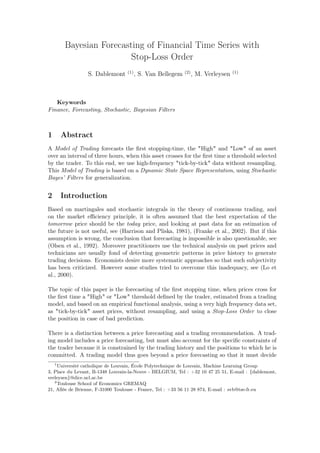
At time t0, see Fig.(1), the Price Forecasting Model forecasts the trend for the next hours.
Based on this trend forecasting, the trader can decide to buy or to sell short a share, or to
do nothing. The Trading model estimates the first stopping time t1 in order to close the
position, depending of a threshold defined by the trader, with a yielding profit.
Figure 1: In the Trading Process we would like to predict the first stopping time, when
prices cross for the first time a threshold defined by the trader.
Two models will be used to realize this objective:
1. for the "Trend" prediction, we use a Price Forecasting Model based on functional
clustering, in which at time t0, we estimate the future trend, and according to this
trend, we realize a trading, buying or selling short an asset;
2. for the "Stopping time" prediction, we use a Dynamic State Space Model and Particle
Filters in which we estimate the stopping time t1, and we close our position at this
stopping time.
In a procedure with "Stop Loss", periodically after time t0 we estimate a new trend. If
this new trend is similar to the former we continue, but if we have a reversal in trend,
immediately we close our position, and we realize an opposite trading, and we rerun the
trading model to get a new stopping time.
2

3. 3.1 Trend Model
The observed time series is split into fixed time-length intervals, for example one day for
regressor, and three hours for prediction. We cannot directly work with these raw data,
we have to realize a functional clustering and a smoothing of these data with splines. We
will work with spline coefficient vectors as variables in our models.
Let be gi(t) the hidden true value for the curve i at time t (asset prices) and gi , yi and
i, the random vectors of, respectively, hidden true values, measurements and errors. We
have:
yi = gi + i, i = 1, · · · , N , (1)
where N is the number of curves. The random errors i are assumed i.i.d., uncorrelated
with each other and with gi.
For the trend forecasting, we use a functional clustering model on a q-dimensional space
as:
yi = Si λ0 + Λ αki + γi + i with k = 1, · · · K clusters. (2)
In these equations:
• yi are the values of curve i at times (ti1, ti2, · · · , tini );
• ini is the number of observations for curve i;
• i ∼ N(0, R); γi ∼ N(0, Γ);
• Λ is a projection matrix onto a h-dimensional subspace with h ≤ q;
• Si = s(ti1), · · · , s(tini )
T
is the spline basis matrix for curve i :
Si =



s1(t1) · · · sq(t1)
...
...
...
s1(tni ) · · · sq(tni )


 . (3)
The term αki is defined as: αki = αk if curve i belongs to cluster k, where αk is a repre-
sentation of the centroid of cluster k in a reduced h-dimensional subspace:
αk = αk1, αk2 . . . αkh
T
. (4)
Then we have :
• s(t)T λ0: the representation of the global mean curve,
• s(t)T (λ0 + Λαk): the global representation of the centroid of cluster k,
• s(t)T Λαk: the local representation of the centroid of cluster k in connection with
the global mean curve,
• s(t)T γi: the local representation of the curve i in connection with the centroid of its
cluster k.
3

4. 3.2 Stopping Time Model
The observed time series is split into fixed time-length intervals of three hours and we
realize a functional clustering and a spline smoothing of this raw data set. We use the
spline coefficient vectors as measurement in a Dynamic State Space model.
In the test phase every day at 11:00 we realize a trading, thus we must run the model every
three hours interval, that means each day at 11:00 and 14:00.
For trading without stop loss, we have regular time intervals of three hours, thus we use
discrete time equations for state and measurements, see Fig.(2).
For trading with stop loss, after the stopping time prediction at 11:00, every ten minutes
we rerun the trend prediction model. According to the result, we could have to rerun
the stopping time model. In this case, we do not have regular time intervals of three
hours anymore, and we must use a continuous time equation for state and a discrete time
equation for measurements, see Fig.(3).
Figure 2: Trading without stop loss. Figure 3: Trading with stop loss.
3.3 Trading Model without "Stop Loss" order
We use a non-stationary, nonlinear Discrete Time Model in a Dynamic State Space repre-
sentation formalized by:
xk = fk(xk−1) + vk (5)
yk = hk(xk) + nk, (6)
For fk and hk functions, we will use a parametric representation by Radial Basis Functions
Network (RBFN) because they possess the universal approximation property, see (Haykin,
1999).
fk(xk) =
I
i=1
λ
(f)
ik exp −
1
σ
(f)
ik
(xk − c
(f)
ik )T
(xk − c
(f)
ik ) (7)
hk(xk) =
J
j=1
λ
(h)
jk exp −
1
σ
(h)
jk
(xk − c
(h)
jk )T
(xk − c
(h)
jk ) . (8)
In these equations:
4

5. • xk is the state, without economic signification,
• yk is the observation, the spline coefficient vector of the smoothing of past raw three
hours data,
• Eq. (5) is the state equation,
• Eq. (6) is the measurement equation,
• vk is the process noise, with vk ∼ N(0, Q),
• nk is the measurement noise, with nk ∼ N(0, R),
• I is the number of neurons in the hidden layer for function fk,
• c
(f)
ik is the centroid vector for neuron i,
• λ
(f)
ik are the weights of the linear output neuron,
• σ
(f)
ik are the variances of clusters,
• J is the number of neurons in the hidden layer for function hk,
• c
(h)
jk is the centroid vector for neuron j,
• λ
(h)
jk are the weights of the linear output neuron,
• σ
(h)
jk are the variances of clusters.
3.4 Trading Model with "Stop Loss" order
We use a non-stationary, nonlinear Continuous-Discrete Time Model in a Dynamic State
Space representation:
dxt = f(xt, t)dt + Lt dβt (9)
yk = hk(xtk
) + nk, (10)
for t ∈ {0, T}, and k ∈ [1, 2, · · · , N] such as tN ≤ T, with non-stationary, nonlinear RBF
functions in state and measurement equations.
f(xt, t) =
I
i=1
λ
(f)
it exp −
1
σ
(f)
it
(xt − c
(f)
it )T
(xt − c
(f)
it ) (11)
hk(xtk
) =
J
j=1
λ
(h)
jk exp −
1
σ
(h)
jk
(xtk
− c
(h)
jk )T
(xtk
− c
(h)
jk ) . (12)
In these equations:
• x(t) is a stochastic state vector, without economic signification,
• yk is the observation at time tk, the spline coefficient vector of the smoothing of past
raw three hours data,
• Eq. (9) is the differential stochastic state equation,
• Eq. (10) is the measurement equation,
• xt0 is a stochastic initial condition satisfying E[||xt0 ||2] < ∞,
5

6. • it is assumed that the drift term f(x, t) satisfies sufficient regular conditions to ensure
the existence of strong solution to Eq. (9), see (Jazwinski, 1970) and (Kloeden and
Platen, 1992),
• it is assumed that the function hk(x(tk)) is continuously differentiable with respect
to x(t).
• nk is the measurement noise at time tk, with nk ∼ N(0, R)
• βt is a Wiener process, with diffusion matrix Qc(t),
• L(t) is the dispersion matrix, see (Jazwinski, 1970).
See (Dablemont, 2008) for a detailed description of these procedures and algorithms.
3.5 How to realize the forecasting
The basic idea underlying these models is to use a Dynamic State-Space Model (DSSM)
with nonlinear, parametric equations, as Radial Basis Function Network (RBFN), and to
use the framework of the Particle filters (PF) combined with the Unscented Kalman filters
(UKF) for stopping time forecasting.
The stopping time forecasting derives from a state forecasting in an Inference procedure.
But before running these models, we must realize a parameter estimation in a Learning
procedure.
3.6 Which tools do we use for stopping time forecasting
The Kalman filter (KF) cannot be used for this analysis since the functions are nonlinear
and the transition density of the state space is non-symmetric or/and non-unimodal. But
with the advent of new estimation methods such as Markov Chain Monte Carlo (MCMC)
and Particle filters (PF), exact estimation tools for nonlinear state-space and non-Gaussian
random variables become available.
Particle filters are now widely employed in the estimation of models for financial markets,
in particular for stochastic volatility models (Pitt and Shephard , 1999) and (Lopes and
Marigno, 2001), applications to macroeconometrics, for the analysis of general equilibrium
models (Villaverde and Ramirez , 2004a) and (Villaverde and Ramirez , 2004b), the ex-
traction of latent factors in business cycle analysis (Billio, et al., 2004), etc. The main
advantage of these techniques lies in their great flexibility when treating nonlinear dy-
namic models with non-Gaussian noises, which cannot be handled through the traditional
Kalman filter.
4 Experiments
4.1 Data
We illustrate the method on the IBM stock time series of "tick data" for the period starting
on January, 03, 1995 and ending on May, 26, 1999. We use the period from January, 04,
1995 to December, 31, 1998 for training and validation of the models, and the period from
January, 04, 1999 to May, 26, 1999 for testing. We use "bid-ask" spreads as exogenous
inputs in the pricing model, and transaction prices as observations in pricing and trading
models
6

7. 4.1.1 Simulation without "Stop Loos" order
Every day, at 11.00 AM, we realize one trading. We decide to buy or to sell short one share
or to do nothing, depending of the trend forecasting; then we close the position according
to the predicted stopping time. We have chosen a threshold of 1 US $. The resulting
behavior of this trading process is presented as a function of time in Fig.(4). The figure of
the cumulative returns includes the losses due to transaction costs (the bid-ask spreads)
but no brokerage fees or taxes. We assume an investor with credit limit but no capital. On
the interval of simulation, Jan, 01, 1999 to May, 26, 1999, we have a positive cumulative
yield, but sometimes we observe a negative local yield. To curb these negative yields we
add a stop-loss process.
4.1.2 Simulation with "Stop Loos" order
We realize one trading, every day at 11.00 AM, and every ten minutes we rerun the pricing
model to estimate the new trend. If this new trend is similar to the former then we
continue, but if we have a reversal in trend we immediately stop and close the position.
We realize a reversal trading (to go short in place of to go long, or the opposite) and rerun
the trading model to predict the new first stopping time in hope to close the position with
a final positive yield. The cumulative returns of this trading process with stop-loss order is
presented as a function of time in Fig.(5). In this simulation, with a stop-loss process, we
have reduced the number of negative local yields and their amplitude. This gives a better
final net yield, but with a very significant increasing of the computational load compared
to the procedure without "stop-loss".
1/4/99 2/1/99 3/1/99 4/1/99 5/1/99 5/26/99
−2
0
2
4
6
8
10
12
14
16
IBM
Dates
Return−US$
Figure 4: Cumulative Returns without
stop-loss order.
1/4/99 2/1/99 3/1/99 4/1/99 5/1/99 5/26/99
0
5
10
15
20
25
30
35
40
45
IBM
Dates
Return−US$
Figure 5: Cumulative Returns with
stop-loss order.
Conclusion
We have presented a functional method for the trading of very high frequency time series by
functional analysis, neural networks, and Bayesian estimation, with Particle and Kalman
filters. A pricing model gives, at time t, a signal of buying or selling short an asset, or
to do nothing. The trader goes long or short. A trading model forecasts when this asset
crosses for the first time a threshold, and the trader closes his position. A stop-loss order
can detect bad forecasting in order to curb the negative local yields. We have realized a
simulation on five months to test the algorithms, and at first sight, the stable profitability
of trading models and the quality of the pricing models could be a good opportunity for
trading assets on a very short horizon for speculators.
7

8. 5 Appendix
5.1 Methodology in Discrete Time
The forecasting procedure in discrete time consists in three phases: "Training" step to fit
models, "Validation" step to select the "best" model according to a criterion and we assess
prediction error using the "Test" step.
We use a "Bootstrap Particle" filter combined with a "Unscented Kalman" filters for pre-
diction of stopping time, in a "Sigma-Point Particle filter".
In an inference procedure, these filters realize a state estimation and a one-step ahead
measurement prediction knowing the parameters of equations. In case of non stationary
systems, we start with a good first initial parameter estimation, and with a joint filtering
((Nelson, 2000)) we can follow the parameter evolution and have a state estimation in the
same step. But when we undergo an important modification of the process dynamic, the
adaptive parameter estimation gives poor estimations and results are questionable. To
get around this problem, periodically we must realize a new parameter initialization in a
batch procedure in two steps: a "Learning" procedure for parameter estimation and an
"Inference" procedure for state estimation, as described in next sections.
5.1.1 Model
Let consider a non-stationary, nonlinear discrete time model in a dynamic state space
representation:
xk = fk(xk−1) + vk (13)
yk = hk(xk) + nk, , (14)
with non-stationary, nonlinear RBF functions in state and measurement equations:
fk(xk) =
I
i=1
λ
(f)
ik exp −
1
σ
(f)
ik
(xk − c
(f)
ik )T
(xk − c
(f)
ik ) (15)
hk(xk) =
J
j=1
λ
(h)
jk exp −
1
σ
(h)
jk
(xk − c
(h)
jk )T
(xk − c
(h)
jk ) . (16)
where
• xk is the state, without economic signification,
• yk is the observation, the spline coefficient vector of the smoothing of past raw three
hours data,
• Eq. (13) is the state equation,
• Eq. (14) is the measurement equation,
• vk is the process noise, with vk ∼ N(0, Q),
• nk is the measurement noise, with nk ∼ N(0, R),
• I is the number of neurons in the hidden layer for function fk,
• c
(f)
ik is the centroid vector for neuron i,
8

9. • λ
(f)
ik are the weights of the linear output neuron,
• σ
(f)
ik are the variances of clusters,
• J is the number of neurons in the hidden layer for function hk,
• c
(h)
jk is the centroid vector for neuron j,
• λ
(h)
jk are the weights of the linear output neuron,
• σ
(h)
jk are the variances of clusters.
5.1.2 Parameter Estimation
In this section, we introduce the general concepts involved in parameter estimation for
stopping time forecasting in discrete time. We only give a general background to problems
detailed in (Dablemont, 2008).
In each training, validation, and test phase, to realize the stopping time prediction, we
need a state forecasting carries out an inference step. This inference step comes after a
parameter estimation in a learning step.
We must estimate two sets of parameters for non-stationary processes, such as:
• estimation of : {λ
(f)
ik , σ
(f)
ik , c
(f)
ik } for function fk(xk),
• estimation of : {λ
(h)
jk , σ
(h)
jk , c
(h)
jk } for function hk(xk).
But, for parameter estimation we need two sets of input and output data:
• for parameter estimation of fk(xk), we need :
– input data {x1, x2, · · · , xk−1, · · · , xN−1}
– output data {x2, x3, · · · , xk, · · · , xN }
• for parameter estimation of hk(xk), we need:
– input data {x1, x2, · · · , xk−1, · · · , xN }
– output data {y1, y2, · · · , yk−1, · · · , yN }
We know measurement {y1, y2, · · · , yk−1, · · · , yN }, but we do not know states
{x1, x2, · · · , xk−1, · · · , xN }. Thus, we cannot directly realize a parameter estimation.
We could use a dual filtering procedure (Nelson, 2000) to estimate, in a recursive proce-
dure, parameters and states. But when the number of parameters and state dimension are
high, this procedure does not stabilize, and we must start the procedure with an initial
parameter estimation.
In next sections, we only sketch the learning and inference procedures for initial parameter
estimation, these procedures and algorithms are detailed in (Dablemont, 2008).
9

10. 5.1.3 Initial Parameter Estimation
To cope with this problem, we realize an initial parameter estimation with EM-algorithm
in a "learning" procedure, and a state estimation by Kalman filters in an "inference"
procedure, into separate steps as follow:
• Learning procedure for stationary, linearized model,
– we consider a stationary, nonlinear system,
– we realize a linearization of equations,
– we use the EM-algorithm to estimate the parameters of the linearized model,
• Inference procedure for stationary, linearized model,
– we use a Kalman smoother for state estimation, using the parameters of the
linearized model,
• Learning procedure for stationary, nonlinear model,
– if we have a small ∆t, the state behaviors of nonlinear and linearized models
are similar, and we can use the state values coming from the linearized model
as input for the nonlinear model, in order to realize its parameter estimation,
Afterwards, we use these initial parameters for the non stationary, nonlinear model, with fk,
and hk functions, in a joint filter procedure, that gives a state prediction and an adaptive
parameter estimation in the training, validation and test phases.
5.1.4 Learning phase for stationary, linearized model
From the non-stationary, nonlinear system, Eq. (13), and (14), we derive the stationary,
nonlinear system:
xk = f(xk−1) + vk (17)
yk = h(xk) + nk, (18)
with stationary, nonlinear RBF functions in state and measurement equations:
f(xk) =
I
i=1
λ
(f)
i exp −
1
σ
(f)
i
(xk − c
(f)
i )T
(xk − c
(f)
i ) (19)
h(xk) =
J
j=1
λ
(h)
j exp −
1
σ
(h)
j
(xk − c
(h)
j )T
(xk − c
(h)
j ) . (20)
We consider a stationary, linearized version of the system:
xk = Axk−1 + vk (21)
yk = Cxk + nk, (22)
where
• xk is the state,
• yk is the observation,
• Eq. (21) is the state equation,
10

11. • Eq. (22) is the measurement equation,
• vk is the process noise, with vk ∼ N(0, Q),
• nk is the measurement noise, with nk ∼ N(0, R).
We estimate the parameters {A, C, R, Q, x0, P0} by EM-algorithm in a learning phase.
5.1.5 Inference phase for stationary, linearized model
From parameters estimated at the precedent step, we estimate the states:
{x0|N , x1|N , · · · , xN−1|N , xN|N }
by the Kalman smoother in an inference phase applied to system given by equations (21),
and (22).
5.1.6 Learning phase for stationary, nonlinear model
We use states given by the precedent step, and observations for a parameter estimation of
RBF functions, Eq. (19), and (20), in a learning phase, that gives the parameters:
{λ
(f)
i , σ
(f)
i , c
(f)
i , λ
(h)
j , σ
(h)
j , c
(h)
j }
5.1.7 Training, Validation and Test Phases
After parameter initialization, we can start training, validation, and test phases using Par-
ticle and Kalman filters.
We consider a non-stationary, nonlinear process and we use the former parameters to realize
the inference procedure for state estimation and curve prediction, such as:
xk = fk(xk−1) + vk (23)
yk = hk(xk) + nk, (24)
with non-stationary, nonlinear RBF functions:
fk(xk) =
I
i=1
λ
(f)
ik exp −
1
σ
(f)
ik
(xk − c
(f)
ik )T
(xk − c
(f)
ik ) (25)
hk(xk) =
J
j=1
λ
(h)
jk exp −
1
σ
(h)
jk
(xk − c
(h)
jk )T
(xk − c
(h)
jk ) . (26)
Every day we want to realize a curve price forecasting for an interval of three hours in an
inference procedure using "Sigma-Point Particle filter". But the system is non stationary,
and parameters depend on time and must be evaluate again in a learning procedure asso-
ciated to an inference procedure.
Starting with a first good initial parameter estimation, we realize both jobs in a joint
procedure, but when we have important dynamic modifications this joint procedure does
not manage this parameter evolution and we have to realize a new parameter estimation
in a batch procedure into two separate steps, as for initial parameter estimation.
11

12. 5.2 Methodology in Continuous-Discrete Time
The forecasting procedure in continuous-discrete time consists in three phases: "Training"
step to fit models, "Validation" step to select the "best" model according to a criterion
and we assess prediction error using the "Test" step. We use a "Continuous-Discrete Se-
quential Importance Resampling" filter, combined with a "Continuous-Discrete Unscented
Kalman" filter for prediction of stopping time.
In an inference procedure, these filters realize a state estimation and a one-step ahead
measurement prediction knowing the parameters of equations. In case of non-stationary
systems, we start with a good first parameter estimation, and with a joint filtering we can
follow the parameter evolution and have a state estimation in the same step. But when
we undergo an important modification of the process dynamic, the adaptive parameter
estimation gives poor estimations and results are questionable. To get around this problem,
periodically we must realize a new parameter initialization in a batch procedure in two
steps: a "Learning" procedure for parameter estimation and an "Inference" procedure for
state estimation, as described in next section.
5.2.1 Model
Let consider a non-stationary, nonlinear continuous-discrete time model in a dynamic state
space representation:
dxt = f(xt, t)dt + Lt dβt (27)
yk = hk(xtk
) + nk, (28)
for t ∈ {0, T}, and k ∈ [1, 2, · · · , N] such as tN ≤ T, with non-stationary, nonlinear RBF
functions in state and measurement equations:
f(xt, t) =
I
i=1
λ
(f)
it exp −
1
σ
(f)
it
(xt − c
(f)
it )T
(xt − c
(f)
it ) (29)
hk(xtk
) =
J
j=1
λ
(h)
jk exp −
1
σ
(h)
jk
(xtk
− c
(h)
jk )T
(xtk
− c
(h)
jk ) . (30)
where:
• x(t) is a stochastic state vector, without economic signification,
• yk is the observation at time tk, the spline coefficient vector of the smoothing of past
raw three hours data,
• Eq. (27) is the differential stochastic state equation,
• Eq. (28) is the measurement equation,
• xt0 is a stochastic initial condition satisfying E[||xt0 ||2] < ∞,
• it is assumed that the drift term f(x, t) satisfies sufficient regular conditions to ensure
the existence of strong solution to Eq. (27), see (Jazwinski, 1970) and (Kloeden and
Platen, 1992),
• it is assumed that the function hk(x(tk)) is continuously differentiable with respect
to x(t),
• nk is the measurement noise at time tk, with nk ∼ N(0, R),
12

13. • βt is a Wiener process, with diffusion matrix Qc(t), for reason of identifiability it is
assumed that Qc(t) is the identity matrix,
• L(t) is the dispersion matrix, see (Jazwinski, 1970),
• I is the number of neurons in the hidden layer for function fk,
• c
(f)
ik is the centroid vector for neuron i,
• λ
(f)
ik are the weights of the linear output neuron,
• σ
(f)
ik are the variances of clusters,
• J is the number of neurons in the hidden layer for function hk,
• c
(h)
jk is the centroid vector for neuron j,
• λ
(h)
jk are the weights of the linear output neuron,
• σ
(h)
jk are the variances of clusters.
5.2.2 Parameter Estimation
In this section, we only give a general background to the general concepts involved in pa-
rameter estimation for stopping time forecasting in continuous-discrete time.
In each training, validation, and test phase, to realize the stopping time prediction, we
need a state forecasting carries out an inference step. This inference step comes after a
parameter estimation in a learning step.
The procedure is similar to the procedure in discrete time, but the complexity is higher
due to a stochastic differential equation for state,
• we must use a quasi-likelihood instead of a real likelihood (Ait-Sahalia, 2002),
• we cannot use EM-algorithm with quasi-likelihood, we must use a direct optimization
with Gauss-Newton procedure (Ait-Sahalia, 2002), and (Nielsen et al., 2000),
• we must realize a discretization of continuous stochastic differential equation (Ait-
Sahalia and Myland, 2003),
• we use Kalman-Bucy filters for initial parameter estimation (Kalman and Bucy,
1961), and (Grewal and al., 2001),
• we use strong solutions for the model (Kloeden and Platen, 1992).
We must estimate two sets of parameters for non-stationary processes, such as:
• estimation of : {λ
(f)
it , σ
(f)
it , c
(f)
it } for function f(xt, t),
• estimation of : {λ
(h)
jk , σ
(h)
jk , c
(h)
jk } for function hk(xtk
).
But, for parameter estimation we need two sets of input and output data:
• for parameter estimation of f(xt, t), we need : {xt} for t ∈ [0, T]
• for parameter estimation of hk(xtk
), we need:
13

14. – input data {xt1 , xt2 , · · · , xtk
, · · · , xtN }
– output data {yt1 , yt2 , · · · , ytk
, · · · , ytN },
We know measurement {yt1 , yt2 , · · · , ytk
, · · · , ytN }, but we do not know states
{xt1 , xt2 , · · · , xtk
, · · · , xtN }. Thus, we cannot directly realize a parameter estimation.
We could use a dual filtering procedure ((Nelson, 2000)) to estimate, in a recursive proce-
dure, parameters and states. But when the number of parameters and the state dimension
are high, this procedure does not stabilize, and we must start the procedure with an initial
parameter estimation.
In next sections, we only sketch the learning and inference procedures for initial parameter
estimation, these procedures and algorithms are detailed in (Dablemont, 2008).
5.2.3 Initial Parameter Estimation
In case of stochastic differential equations, we cannot use the EM algorithm, see (Ait-
Sahalia, 2002), and (Nielsen et al., 2000). To cope with this problem, we realize an initial
parameter estimation with a Gauss-Newton optimization in a "learning" procedure, see
(Kim and Nelson, 1999), and a state estimation by Kalman-Bucy filters in an "inference"
procedure, into separate steps.
We sketch the methodology for initial parameter estimation.
• We transform the stochastic differential equation with Wiener process into a stochas-
tic differential equation with white noise (Jazwinski, 1970),
• Learning procedure for stationary, linearized model,
– we consider a stationary, nonlinear system,
– we realize a linearization of equations,
– we use the Gauss-Newton algorithm to estimate the parameters of the linearized
model (Bjorck, 1996), and (Fletcher , 1987),
• Inference procedure for stationary, linearized model,
– we use a Kalman-Bucy smoother for state estimation, using the parameters of
the linearized model,
• Learning procedure for stationary, nonlinear model,
– if we have a small ∆t, the state behaviors of nonlinear and linearized models
are similar, and we can use the state values coming from the linearized model
as input for the nonlinear model, in order to realize its parameter estimation,
5.2.4 Training, Validation and Test Phases
After initial parameter initialization, we can start training, validation, and test phases
using stochastic Particle filters and Kalman-Bucy filters in continuous time.
We consider a non stationary, nonlinear process and we use the former parameters to realize
the inference procedure for state estimation and curve prediction.
dxt = f(xt, t)dt + Lt dβt (31)
yk = hk(xtk
) + nk, (32)
14

15. for t ∈ {0, T}, and k ∈ [1, 2, · · · , N] such as tN ≤ T, with non-stationary,nonlinear RBF
functions in state and measurement equations:
f(xt, t) =
I
i=1
λ
(f)
it exp −
1
σ
(f)
it
(xt − c
(f)
it )T
(xt − c
(f)
it ) (33)
hk(xtk
) =
J
j=1
λ
(h)
jk exp −
1
σ
(h)
jk
(xtk
− c
(h)
jk )T
(xtk
− c
(h)
jk ) . (34)
Every day we want to realize a curve price forecasting for an interval of three hours in
an inference procedure using a "Continuous-Discrete Unscented Kalman Filter", and a
"Continuous-Discrete Sampling Importance Resampling Filter". But parameters depend
on time and must be evaluate again in a learning procedure associated to an inference
procedure.
Starting with a first good initial parameter estimation, we realize both jobs in a joint
procedure, but when we have important dynamic modifications this joint procedure does
not manage this parameter evolution and we have to realize a new parameter estimation
in a batch procedure into two separate steps, as for initial parameter estimation.
5.3 Functional Clustering Model
For the trend forecasting, we use a functional clustering model on a q-dimensional space
as:
yi = Si λ0 + Λ αki + γi + i with k = 1, · · · K clusters. (35)
We have to estimate the parameters λ0 , Λ , αk , Γ , σ2 et πk by maximization of a
likelihood function.
For yi we have a conditional distribution :
yi ∼ N Si(λ0 + Λαki), Σi , (36)
where
Σi = σ2
I + SiΓST
i . (37)
We define zi as the unknown cluster membership vector of curve i, which will be treated
as missing data,
zi = z1i z2i · · · zki · · · zGi (38)
with :
zki =
1 if curve i belongs to cluster k,
0 otherwise.
The probability that curve i belongs to cluster k is then :
πki = P zki = 1 . (39)
If the γi were observed, the joint likelihood of yi, zi and γi would simplify. As zi and γi
are independent, the joint distribution can be written as :
f(y, z, γ) = f(y|z, γ)f(z)f(γ) , (40)
where for each curve i,
15

16. • zi are multinomial (πk),
• γi are N(0, Γ),
• yi are conditional N Si(λ0 + Λαk + γi); σ2I .
The joint distribution is now written as :
f(y, z, γ) =
1
(2π)
n+q
2 |Γ|
1
2
exp −
1
2
γT
Γ−1
γ
G
k=1
πk exp −
1
2
n log(σ2
)
exp −
1
2σ2
y − S(λ0 + Λαk + γ)
T
y − S(λ0 + Λαk + γ)
zk
,
(41)
and the likelihood of the parameters is given by :
L(πk, λ0, Λ, αk, Γ, σ2
|y1:N , z1:N , γ1:N ) =
N
i=1
1
(2π)
ni+q
2 |Γ|
1
2
exp −
1
2
γT
i Γ−1
γi
G
k=1
πk exp −
1
2
ni log(σ2
)
exp −
1
2σ2
yi − Si(λ0 + Λαk + γi)
T
yi − Si(λ0 + Λαk + γi)
zki
.
(42)
For parameter estimation by EM algorithm, we will use the log likelihood:
l(πk, λ0, Λ, αk, Γ, σ2
|y1:N , z1:N , γ1:N ) =
−
1
2
N
i=1
(ni + q) log(2π)
+
N
i=1
G
k=1
zki log(πk) (43)
−
1
2
N
i=1
log(|Γ|) + γT
i Γ−1
γi (44)
−
1
2
N
i=1
G
k=1
zki ni log(σ2
) +
1
σ2
yi − Si(λ0 + Λαk + γi)
2
. (45)
————————————————————————————————————–
5.3.1 Algorithm - Learning - Functional Clustering EM algorithm
The EM algorithm consists in iteratively maximizing the expected values of (43), (44) and
(45) given yi and the current parameters estimates. As these three parts involve separate
parameters, we can optimize them separately.
Initialization
First, we must initialize all parameters:
{λ0, Λ, α, Γ, σ2
, zik, πk, γi}.
E-step
The E-step consists in :
γi = E γi|yi, λ0, Λ, α, Γ, σ2
, zik . (46)
16

17. with:
γi = ST
i Si + σ2
Γ−1 −1
ST
i yi − Siλ0 − SiΛαk . (47)
M-step
The M-step involves maximizing :
Q = E l(πk, λ0, Λ, αk, Γ, σ2
|y1:N , z1:N , γ1:N ) , (48)
holding γ1:N fixed, and given by the E-step.
The steps of this algorithm are detailed in (Dablemont, 2008).
—————————————————————————————————————
References
Ait-Sahalia, Y., and P.A. Myland,(March,2003), ”The effects of random and discrete sam-
pling when estimating continuous-time diffusions”, Econometrica, Vol. 71, pp.483-549.
Ait-Sahalia, Y.,(january,2002), ”Maximum likelihood estimation of Discretely sampled Dif-
fusions: a Closed-orm approximation Approach”, Econometrica, Vol. 70, pp. 223-262.
Billio, M., R. Casarin, and D. Sartore ,(2004), ”Bayesian Inference on Dynamic Modelss
with Latent Factors”, in Official Monography, Edited by EUROSTAT.
Bjorck, A., (2007), ”Numerical methods for least squares problems” (SIAM)
Dablemont, S. ”Forecasting of High Frequency Financial Time series”, PhD thesis,
Université catholique de Louvain - Belgium, 2008. http://edoc.bib.ucl.ac.be:81/ETD-
db/collection/available/BelnUcetd-11172008-174432/unrestricted/these.pdf
Bjorck, A., (2007), ”Practical methods of optimization” ( John Wiley & Sons)
Franke, G., R. Olsen and W. Pohlmeier,(June 2002), ”Overview of Forecasting Models”,
University of Konstanz, Seminar on High Frequency Finance, paper SS 2002.
Grewal, M.S., and A.P. Andrews,(2001), ”Kalman Filtering: Theory and Practice. Using
MATLAB”, John Wiley & Sons .
Harrison, J.M., S.R. Pliska ”Martingales and Stochastic integrals in the Theory of Conti-
nous trading”, Stochastic Processes and their Applicartions, Vol. 11, Pp. 215-260, 1981.
Haykin, S.,(1999), ”Neural Networks - A comprehensive foundation”, Prentice Hall,
Jazwinski A.H.,(1970), ”Stochastic Processes and Filtering Theory”, Academic Press.
Kalman, R.E. ”A new approach to linear filtering and prediction problems”, Transactions
of the ASME, Journal of basic Engineering, Vol. 82, pp. 34-45, March 1960
Kalman, R.E. and R.S. Bucy (1961) ”New results in linear filtering and prediction theory.”,
Transactions of the ASME, Journal of basic Engineering, Vol. 83, pp. 95-108, 1961
Kim, C.J.,and M. Nelson ”State-space Models with regime-Switching: Classical and Gibbs
Sampling Approach with Applications”, MIT Press 1999.
Kloeden, P.E. and E. Platen, ”Numerical Solution of Stochastic Differential Equations”,
Springer-Verlag.
17

18. Lo, A.W., H. Mamaysky, and J. Wang ”Foundations of Technical Analysis : computation
algorithms, statistical inference, and empirical implementation”, Journal of finance, Vol.
55, pp. 1705-1765, 2000
Lopez, H.F., and C. Marigno,(2001), ”A particle filter algorithm for the Markov switching
srtochastic volatility model”, Working paper, University of Rio de Janeiro.
Nelson, A.T.. ”Nonlinear Estimation and modeling of Noisy Time-Series by dual Kalman
Filtering Methods”, PhD thesis, OGI School of Science and Engineering, Oregon Health
and Science University, 2000.
Nielsen, J.N., H. Madsen and H. Melgaard,(2000), ”Estimating Parameters in Discretely,
Partially Observed Stochastic Differential Equations.”, Technical University of Denmark.
Olsen, R.B., M.M. Dacorogna, U.A. Muller and O.V. Pictet ,(1992), ”Going Back to the
Basics Rethinking Market Efficiency”, Olsen and Associates Research Group, RBO. 1992-
09-07 December 2, 1992.
Pitt, M., and N. Shephard ,(1999), ”Filtering via Simulation : Auxiliary particle Filters”,
Journal of the American Statistical Association, Vol. 94(446), pp.590-599.
Villaverde, J.F., and J.F. Ramirez,(2004b), ”Estimating nonlinear Dynamic Equilibrium
Economies: Linear versus Nonlkinear Likelihood”, Atlanta FED, Working paper N. 01.
Villaverde, J.F., and J.F. Ramirez,(2004a), ”Estimating nonlinear Dynamic Equilibrium
Economies: A likelihood Approach”, Atlanta FED, Working paper N. 03.
18