1. CHE255 PROJECT REPORT
To: Professor Doug Kelley, Department of Chemical Engineering, University of Rochester
Team Macomb: Jon Drake, Yatong Ge, Robert Harding, Jennifer Reisfeld
Title: Analysis of Heat Exchange Properties of Small Scale Stirling Engines
Abstract:
The Stirling Engine is a promising technology for alternative energy due to its zero carbon emissions. It is
an engine that derives its power from an external heat source,assuming that there is a substantial
temperature difference between the engine and the environment. Up until this point little research has
been performed on heat exchange properties of Stirling Engines. Efficient electricity and power
production within the Stirling Engine depends upon efficient heat transfer between the cylinder and the
working fluid. In this experiment, the material properties of low temperature Stirling Engines were
studied. Specifically, this study focused on the ways that efficiency and performance (measured by the
number of revolutions per minute) were affected by the materials used and their corresponding thermal
conductivities, the working fluid inside of the engine’s piston, and the addition of fins to the cold side of
the engine. The studies show that thermal conductivity of the heat exchangers and the thermal diffusivity
of the working fluid have significant impacts on the performance of the Stirling Engine. Heat exchangers
made of copper, aluminum, steel, and stainless steelwere tested and it was found that at 45 degrees
Celsius, a copper heat exchanger yielded the worst engine performance while at 85 degrees,it had by far
the best performance. The experiments also found that using helium as a working fluid produced a higher
performing engine than that of air or carbon dioxide. This supports the notion that thermal diffusivity is
linearly related to the engine’s performance. Lastly, the addition of fins to the engine proved to have no
significant benefit on the low temperature Stirling Engines. The findings of this experiment are found
below and can be used to determine the heat transfer properties of the Stirling Engine that lend itself to
the most efficient and best performing engine.

2. 2
Introduction:
The Stirling Engine is an old technology that has recently been revived due to its promising potential as a
source of Green Energy. It is a heat engine, meaning that heat or thermal energy is converted to
mechanical energy which is then used to do some type of work. In the case of the Stirling Engine, heat
from an external source is required in order to expand the working fluid inside of the piston so that work
can be produced.
Although the Stirling Engine is a heat engine, it differs greatly from other heat engines, specifically that of
the Carnot Engine. The Carnot Engine represents the ideal heat engine and consists of two isothermal and
two adiabatic processes. The Carnot cycle sets the limit on the amount of heat from the engine that can be
used to do work assuming that the process is reversible and that no change in entropy occurs. Based on
the mere fact that engines cannot be completely reversible, the Carnot Engine is an idealization of the
most efficient engine and therefore the Carnot efficiency represents the maximum efficiency that any heat
engine can achieve. However,unlike the Carnot Engine which is composed of two isothermal and two
adiabatic processes,the Stirling Engine is composed of two isothermal and two isometric processes. The
difference between these two cycles results in differences in calculations of the overall work, heat
transfer,and efficiency that is achieved throughout the cycle.
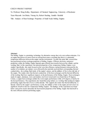
The figure above represents the ideal Stirling Engine cycle and the various processes that occur
throughout it. Starting at point 1, the Stirling Engine experiences isometric heat transfer in order to move
to point 2. During this process,Qheat is added to the system at constant volume causing both the
temperature and pressure to rise. Once at point 2 and a temperature of TH, the engine experiences
isothermal expansion. As seen on the figure above, this isothermal expansion phase requires the input of
heat, Qexp, and produces work, Wexp , as the piston is pushed forward allowing the working fluid to
expand. From point 3, the engine then experiences isometric heat rejection or cooling. During this
process,the system once again remains at constant volume. However, unlike the isometric heat transfer
phase where heat was added, this stage results in a loss of heat, Qcool,as the working fluid is cooled from
TH to TC. Lastly, in order to return to the starting point of the cycle, isothermal compression occurs. This
compression requires that work is supplied in order to pull the piston back and compress the working fluid
and also results in a loss of heat, Qcomp.
Based on the figure above, thermodynamics can be used to determine equations for work, heat transfer
and efficiency for a Stirling Engine. The net work for a Stirling Engine is defined as the work of
expansion plus the work of compression. Using the ideal gas law and plugging it into equation 1, the net
work of a Stirling Engine can be calculated and is shown below in equation 2.
Figure 1: StirlingEngine

3. 3
Wnet = Wexp+ Wcomp=∫exp PdV +∫comp PdV Eq. 1
Wnet=nR(TH-TC)ln(V1/V0) Eq. 2
The same concept that was used to find the work can be used to find the total heat applied to the engine or
Qtot. Knowing that total heat provided to the engine is given by the sum of Qheat and Qexp, the expression in
equation 3 can be obtained.
Qtot= Qexp+ Qheat = ∫expPdV +Qheat Eq. 3
Substituting in the expression for the work of expansion and the heat added, equation 4 can then be
achieved.
Qtot= nRTHln(V1/V0) + nCv(TH-TC) Eq. 4
Once the expressions for the net work and total heat have been determined, the efficiency of the engine
can be obtained. The efficiency is defined as the ratio of net work to the total heat of the engine.
Substituting in the expressions that were obtained for the net work and total heat into equation 5 below,
the ideal Stirling Engine efficiency can be calculated and is shown in equation 6.
η = Eq. 5
ηS = Eq. 6
Given that the Carnot efficiency is defined by equation 7 below, it can be seen that the Stirling Engine
efficiency will always be less than that of the Carnot efficiency.
η = Eq. 7
It is important to note that although the Stirling Engine efficiency depends on the temperature difference
between the hot and cold plate as it does in the Carnot efficiency, the Stirling efficiency is also dependent
on other factors such as the specific heat capacity of the working fluid and the volume ratio between the
compression and expansion of the working gas. Therefore, in Stirling Engine analysis, it is important to
look at a variety of factors that can impact the efficiency of the engine by altering heat transfer properties.
Within the Stirling Engine, the difference in temperature is the driving force for the engine to operate. In
the analysis of the Stirling Engine performance and efficiency, heat transfer by conduction and convection
become significant factors that contribute to differences in these values. Heat transfer by conduction occurs
by molecular agitation within a fluid and is present as heat is transferred throughout a material. With
conductive heat transfer,it is essential that a thin material with a high thermal conductivity is used in order
to ensure fast and efficient heat transfer. Due to the fact that the overall heat transfer by conduction is
dependent on the thermal conductivity of a material (k) as seen below in equation 8, different materials will
yield unique results for the performance (measured in revolutions per minute, RPM) and efficiency of the
engine.
q= ΔT Eq. 8

4. 4
Heat transfer by convection also has a significant effect on the engine’s efficiency and performance. Heat
transfer by convection is defined by the transfer of thermal energy from one place to another by the
movements of fluids and occurs as heat is transferred from a surface or wall to a working fluid. Within the
Stirling Engine, heat transfer by convection occurs as the hot plate transfers heat to the working fluid as
well as when the working fluid transfers heat to the cold plate. Noting equation 9 below, one notices that
maximizing convective heat transfer (q) requires increasing the temperature difference (ΔT),the surface
area (A),or the heat transfer coefficient (h).
q= hAΔT Eq. 9
In the experiments discussed below, the effect of convective heat transfer was analyzed by varying the
working fluid inside of the engine’s piston. Due to the fact that the heat transfer coefficient is proportional
to the thermal conductivity of the working fluid as seen in equation 10 below, it is expected that fluids
with different thermal conductivities will run at different efficiencies and performances. Throughout this
experiment, three working fluids with a range of thermal conductivities were used in order to test the
theory which states that a fluid with a higher thermal conductivity will yield a higher heat transfer
coefficient, and thus it is expected that the overall heat transfer,q, will increase.
h= Nu*kl Eq. 10
The addition of fins to the cold side of the Stirling Engine are thought to also have an impact on the way
that the engine operates and how efficiently it runs. Fins are surfaces that extend from an object to
increase the rate of heat transfer to or from the environment. Fins increase the amount of convection and
thus increase the rate of heating or cooling of an object. In order to be effective, it is essential that the fins
are optimized for the system so that maximum heat transfer can be achieved. Therefore,not only do
various fin dimensions impact the system, but the spacing between the fins also will affect how efficient
the fins operate.
Throughout this experiment, tests were run on the Stirling Engines in order to determine optimal heat
transfer conditions that yield the greatest performance and efficiency. The effect of various heat
conductors including copper, stainless steel, steel, and aluminum were tested. Different working fluids
including air, helium and carbon dioxide were introduced to the engine in a bell jar and their impact on
how the engine ran was studied. Lastly, the experiments described below looked at the impact that fins
have on the performance and efficiency of the engines in order to determine if the addition of fins yielded
more optimal heat transfer conditions.
Experimental Methods and Procedures:
To perform this experiment, four low temperature Sunnytech Stirling Engines were used. These engines
were modified in the machine shop by John Miller in order to be able to test various heat conduction
materials throughout the trials. The engines were modified so that there were four engines made of four
different materials: steel, copper, stainless steel, and aluminum. During the modification in the machine
shop, the piston cylinders were reconstructed with granite due to cracking of the original glass cylinders.
To run the various experiments, a heater was needed in order to control the heat load supplied to the hot
side of the engine. For the heat conduction experiments a cylindrical heater was used while for the
working fluid and fin experiments, a flat heater was used. The heaters were interfaced to a solid state
relay and a measuring computing board so that the heat load could be controlled. A LabVIEW program
that incorporated Proportional and Integral Control (PI) was written and used throughout all experiments.
This LabVIEW program also included pulse wave modulation in order to yield better control of the heater
as well as code for counting using an optical sensor so that the performance (revolutions per minute)
could be recorded. A screenshot of the front panel of the final LabVIEW Program can be seen in the
figure below.

5. 5
Figure 2: Front Panel of LabVIEW program
As seen on the figure above, a temperature set point for the heater was used. The error between the set
point temperature and the actual heater temperature was minimized through the use of PI control and
pulse width modulation. The conditions for pulse width modulation are shown at the bottom of the figure.
Depending on how large the error was,the control output for PI control was further limited in order to
turn the heater on for a shorter amount of time. As the Stirling Engine operated,two graphs were created.
The first graph displays the various temperatures that were collected throughout the trials as well as how
well the heater was being controlled. The bottom graph shows the number of RPMs that the engine was
operating at for the given set point temperature. This LabVIEW program was used for all of the
experiments conducted in order to gather and analyze the data.
When running experiments, three thermocouples were used. A thermocouple was placed directly on the
heater,on the hot side of the engine and on the cold side of the engine. The wires of these thermocouples
were connected to the measuring computing board with the heater connected to channel 0, the hot side
connected to channel 1, and the cold side connected to channel 2. After connecting the thermocouples, the
Stirling Engine was placed on top of the heater. An apparatus was used (clamp stand or Legos) in order to
hold the optical sensor in place at the correct height. Once assembled, the Stirling Engine was positioned
so that its flywheel was inside of the prongs of the optical sensor in order to measure performance and the
engine was started and began to run. The optical sensor was connected to a LabJack and the counting
function was utilized in order to record the number of RPMs of the engine. Both the LabJack and the
measuring computing board were interfaced to the computer and the LabVIEW program was run in order
to collect data during the experiments. The LabVIEW program was wired to write to an excel file and
after each trial, the temperature of the heater,the hot plate and the cold plate, as well as the number of
RPMs and the time were recorded. The generalsetup of this experiment is shown below in figure 3.

6. 6
Figure 3: Experimental Setup on FlatPlate Heater
To thoroughly analyze the Stirling Engine efficiency and performance, three different studies were
performed. The first study that was conducted focused on changing the heat conduction properties of the
engine. For this experiment, the four different low temperature engines (steel, copper, stainless steel, and
aluminum) were tested at five temperatures:45, 50, 55, 60, and 85 degrees Celsius. The LabVIEW
program was used to control and modify the heater temperature for each trial with the use of PI control.
The proportional and integral constants were varied until good control was achieved. Once the constants
were found, the program was run and the engine was placed on top of the heater. The engine was started
and the LabVIEW program recorded the essential data for the analysis of the Stirling Engine. For this
experiment, each engine was tested three times at the temperatures listed above in a randomly allocated
execution order. Between each trial run, the engine was allowed to cool back down to room temperature.
For the second study, the stainless steel engine was run in a bell jar. In order to run this experiment,
various materials and components were needed. A flat plate was constructed out of plastic and used so
that the engine would sit on the plate inside of a desiccator and would be sealed from the outside air. The
flat plate was machined so that there was a divot on the side for the various wires to sit in while ensuring
the bell jar was sealed. The plate also included barb fitting for the new working fluid to enter and for the
air to exit the jar. Tubes were used to move the working fluid in and out of the jar as a tube was run from
the gas tank and connected to the barb fitting. For these experiments, three working fluids were tested:air,
helium and carbon dioxide. For the helium trials, the engine was tested at 50, 55, and 60 degrees where as
for the air and carbon dioxide studies, the engine was tested at 55, 60, and 70 degrees. The engine was run
at each temperature twice, for a total of six trials per working fluid.
For the third and final study, fins were added to the cold side of an engine in order to see what effect they
have on the engine’s performance and efficiency. After designing fins with the use of an optimization
program, the fins were produced in the machine shop. The fins were made out of aluminum and were on a
plate that could slide on top of the cold side of the engine. Due to the fact that the fins were constructed
out of aluminum, the aluminum engine was used during these experiments in order to provide a good
comparison to the trials run without fins. The fins were attached to the engine with the use of thermal
paste. The engine was tested with fins at three temperatures:45, 60, and 85 degrees in order to compare
the efficiency and performance with and without fins. The engine was run three times at each of the
temperatures above.
After all experiments and trials were completed, the data was analyzed in order to compare the
efficiencies and performances between experiments. The analysis of the data included determining the
Carnot efficiency, the Stirling efficiency, the number of RPMs,and finding the amount of heat transfer
that occurred throughout the engine.

7. 7
Heat Conduction Experiments:
The first of our series of three experiments was designed to test the influence thermal conductivity of
various heat exchanger materials has on the heat transfer across the entire engine. The materials selected
were chosen based on their affordability and large range of thermal conductivities in order to see the
clearest results from our experiments while still being pragmatic. These materials and their significant
characteristics are listed in the following table.
Table 1: Heat Exchange PropertiesofVarious Materials
Heat Exchange Materials Thermal Conductivity Thermal Diffusivity
Copper 385 W/m-K 1.11*10-4
m2
/s
Aluminum 205 W/m-K 8.44*10-5
m2
/s
Steel 50.2 W/m-K 1.44*10-5
m2
/s
Stainless Steel 18 W/m-K 4.52*10-6
m2
/s
Thermal conductivity was determined to be the most important parameter to the experiment according to
the equation for heat transfer by conduction (equation 8), where the rate of heat transfer is dependent on
the thermal conductivity of the material while all other parameters are fixed in the experiment. These
materials were tested under controlled conditions with the engine running at a steady-state temperature
profile for an extended period of time. The engine performance would vary significantly with small
changes in temperature to both the hot and cold side of the heat exchanger. Thus to ensure accuracy,each
test was performed for approximately 20-30 minutes with down time between trials to allow for the
cooling of both the engine and the heater.
Figure 4: Average Carnot efficiencies for all materials and temperatures tested

8. 8
Figure 5: Average Stirling efficiency for all materials and temperatures tested
The Stirling and Carnot efficiencies were calculated for every trial according to equations 6 and 7
respectively. These two calculations help illustrate how the engine’s optimal performance increases in
proportion to the amount of temperature input due to the heat exchanger’s ability to establish a larger
temperature gradient for the working fluid. These figures (shown above) can be compared to the four
engines performances across the various temperatures in order to see which material can produce the most
mechanical work relative to both its Carnot and Stirling efficiencies.
Figure 6: Average engine performance across all trials
As expected,all engine performances increased with increasing temperature input from the heater,but at
varying rates. Stainless steel and steel, the two poorest thermal conductors, performed arguably the best
when the engines were being operated at the near minimum required temperature difference for ambient
conditions. Yet at higher temperatures,both copper and aluminum, the best two conductors, performed

9. 9
significantly better, especially copper which expressed the most drastic change in mechanical output
across the tested temperature range. The difference in thermal energy being transferred to the working
fluid is subtle but does increase with higher temperatures. This could explain copper’s dramatic increase
in performance when the engines were tested at near maximum temperatures. Copper at all temperatures
should be the best option for hot side of the heat exchanger due to its high thermal conductivity but its
high conductivity could also explain its high performance as a cold side heat exchanger for the Stirling
Engine.
In order to more directly compare the performances of the cold side heat exchangers,the best and worst
conductors (copper and stainless steel) were tested using the same material as the hot side heat exchanger.
Figure 7: Results of the stainless steel vs. copper as the cold side of the heat exchanger experiment
Across all temperatures, the stainless steelcold side engine performed better than that of the copper cold
side engine. The figure above shows that for low temperatures,the copper plate is a poorer heat sink for
the engine than stainless steel. This suggests that poorer thermal conductors make better heat sinks than
materials with high thermal conductivities. This finding could explain the observation that the copper
engine had the worst performance than the other three engines at lower temperatures during the previous
trials. Therefore,it appears that the cold side of the heat exchanger has a greater impact than the hot side
at lower temperatures.
Working Fluid:
For the working fluid experiments, new working fluids with varying thermal conductivities were injected
into the bell jar and slowly filled in and diffused into the engine’s piston. The working fluids chosen were
air, helium, and carbon dioxide in order to gather data from a range of thermal conductivities. For air and
carbon dioxide, the engine was tested at 55°C, 60°C, and 70°C while for helium, the engine was tested at
50°C, 55°C and 60°C. The discrepancy in the testing temperatures is due to the fact that the air and
helium engines would not run at the lower temperatures. A picture of the bell jar setup is shown below in
figure 8. For each trial performed, the engine ran for 30-40 minutes to ensure that the new working fluid
diffused into the engine and that the engine’s performance stabilized. Between trials, the engine’s plates
were allowed to cool to room temperature for experimental consistency. The data was then analyzed and
efficiency and RPM values were compared to show the following results.

10. 10
Figure 8: Bell Jar Set-up
Working Fluid Results:
After performing the experiments where new working fluid was injected into the bell jar, the data was
analyzed and the following charts were obtained.
Figure 9: Average Carnot Efficiency for Different Figure 10: Average RPM for Different Temperatures for
Temperatures for Helium and Air Helium and Air
From the figures above, it can be noted that the Stirling Engine with helium as working fluid had around a
30% Carnot efficiency while the engine with air had an approximately 5% higher Carnot efficiency for all
experiments. However,the Stirling Engine with helium had a much higher number of RPMs than the
engine with air when comparing RPM values at 55 and 60 degrees Celsius. The engine with helium also
showed much greater improvement in the number of RPMs as the temperature increased in comparison
with that of air. As seen on the figures above, the engine with air did not run at a temperature of 50
degrees Celsius as the temperature difference between the heat source and heat sink was not significant.
The results shown on the figures above were expected due to the varying thermal diffusivity of the
working fluids. Thermal Diffusivity is proportional to thermal conductivity and inversely proportional to
(°C) (°C)

11. 11
density and specific heat. The heat equation which describes the distribution of temperature over time is
shown below in equation 11. As seen from this equation below, the heat distribution is dependent on the
thermal diffusivity of the working fluid that is present.
Eq. 11
According to values obtained in literature, helium has a higher thermal conductivity and a lower density
than air, thus having an obvious advantage in thermal diffusivity. As the helium engine ran, the cold plate
temperature increased at a faster rate due to the fact that the helium engine is able to produce more work
which as a result generates more heat from the engine and lowers the Carnot efficiency. This relationship
between performance speed and thermal diffusivity is very evident in figure 10 above. As noted in Table
2 below, the thermal diffusivity is about ten times greater than that of air. When looking at the above
figures, it can be noted that the helium engine performed about seven to eight times better than that of air
which is a direct result of the higher thermal diffusivity value. The discrepancy in these values could be a
result of the variations in Carnot efficiency.
Table 2: Values for thermal conductivity and thermal diffusivity for the various working fluids
Working Fluid Thermal Conductivity
(W/m-K)
Density
(kg/m3
)
Specific Heat
(J/kg-K)
Thermal
Diffusivity (m2
/s)
Helium 0.138 0.164 5188 1.62*10-4
Air 0.024 1.225 1010 1.94*10-5
Carbon Dioxide 0.0146 1.98 844 8.74*10-6
After injecting the stainless steelStirling Engine with helium, carbon dioxide was then injected into the
bell jar and the engine was allowed to run. As seen on figure 11 below, the Stirling Engine running on
carbon dioxide had a higher Carnot efficiency than that of air at all temperatures tested. It can also be seen
from figure 12, below, that once carbon dioxide had enough time to diffusive into the engine and
stabilize, the engine running on carbon dioxide had a lower number of RPMs than that of air at 70 degrees
Celsius.
Figure 11: Average Carnot Efficiency for Different Temperatures for Carbon Dioxide
and Air
(°C)

12. 12
Figure 12: RPM vs. Time at 70°C for Carbon Dioxideand Air
It is important to note that while data was collected for carbon dioxide at 55 and 60 degrees Celsius, the
engine did stop running multiple times. However,this did not hinder the collection of data and the ability
to show that since carbon dioxide was operating more slowly due to its low thermal diffusivity, less work
was being produced and thus less heat was created therefore leading to a higher Carnot efficiency for all
trials.
Error Analysis Working Fluid Experiment:
While the results obtained during these trials were statistically significant in showing that a working fluid
with a higher thermal diffusivity (such as helium) could improve engine performance,there was some
error associated with these experiments. One source of error throughout this experiment could be related
to the injection of the working fluid inside of the bell jar. For both carbon dioxide and helium, the gas was
injected continuously throughout all trials. However,for the trials with air run in the bell jar, there was no
continuous flow of gas into the bell jar and thus more heat could have been trapped in these trials.
Another source of error that was present during this experiment was related to where the gas injection
occurred. For all trials, the gas was injected through a small hole at the bottom of the jar and the air left
through a similar hole on the opposite side. This was the ideal configuration for helium since it is lighter
than air. However,carbon dioxide is heavier than air and thus as shown in the figure above, it took a
much longer time for it to diffuse into the engine. Ideally, carbon dioxide gas would have entered from
the top of the bell jar. However,due to limitations in the equipment used, the set up could not be modified
to account for this difference. Yet,even with the error present, the results from this experiment were
conclusive in showing that working fluids with higher thermal conductivities and diffusivities have a
higher performance than those fluids with lower values.
Fin Experiment Optimization:
Fins are attached to heatsinks to improve the heat transfer between a solid and a fluid. If a surface is in
contact with a fluid, the heat transfer between the mediums is governed by the convective heat transfer
equation (Equation 9). It is seen that the contact area is linearly proportional to the convective heat
transfer. Since fins increase the area of the heat sink, fins can enhance the cooling of a surface. An Excel
program was developed to assist in optimizing the dimensions of the fins. Details of the program may be
found in the Appendix; a surface plot of the results and a description of the found dimensions are shown
in figure 13 and Table 3 below.

13. 13
Table 3: Optimal Fin
Dimensions
Figure 13: SurfacePlot for Optimal Fin Dimensions
For ease of calculation, these dimensions were found by approximating the circular engine top as a
square. The dimensions of the actual plate therefore differ slightly from the above dimensions. The
surface area of the fin plate was measured with a micrometer and compared with the surface area of the
unaltered engine top. The addition of fins increased the surface area by approximately 1.66%. The areas
are shown below in Table 4.
Table 4: Surface Area of Plate with and without Fins
Surface Area of Fin Plate (mm2
) 13874.5
Surface Area of Engine Top (mm2
) 8364.7
The fin plate and the engine with the attached fins can be seen in figure 14 below. To ensure good contact
between the engine top and the fin plate, and to promote heat transfer between the two, a thermal paste
with a zinc oxide base was applied.
Length (Fixed) 105 mm
Height 10 mm
Width 1 mm
Space Between Fins 10 mm
Number of Fins 9

14. 14
Figure14: Fin Plateboth attached and detached from the engine
Fin Experimental Results:
For the fin experiments, the RPMs at each temperature with fins was compared to the RPMs from the
same engine without fins. Another set of trials was executed where a small fan was used to examine the
effect of forced convection on the engine performance. The results of these experiments are shown below
in figure 15.
Number of RPMs vs. Heater Control for Various Fin
Set-ups
45° 60° 85°
Heater Control Temperature (°C)
Figure 15: Chart of RPMs with various fin set-ups
The similarity in results between trials justified executing an unpaired t test to determine statistical
significance. It was determined that these results are not statistically significant within a 95% confidence
interval. The fin addition did not yield an enhanced performance.
Error Analysis Fin Trials:
There was some inconsistency between trials that may have attributed towards the insignificant findings
from the fin experiments. The thickness of the fin plate was initially overlooked but is now seen as a
source of error. A thermocouple placed in the well of the fins indicated that the base temperature of the
fin was severaldegrees colder than the temperature of the cold plate without fins. These findings are
summarized in Table 5. It is believed that the additional 3.2 mm of the fin plate dissipated much of the
heat prior to it reaching the fins. This rendered the fins essentially useless for this low temperature Stirling
Engine. However,fins may be more effective when there is a larger temperature gradient between the
0
50
100
150
200
250
300
350
fins and air
no fins
fins no air

15. 15
cold plate and the cooling fluid- air at 19°C. If the cold plate was hotter or if the cooling fluid were ice or
chilled water,it is likely there would be a benefit to adding fins.
TABLE 5: Average Cold Plate Temperature with and without fins
Heater Temperature (°C) Cold Plate- No Fin average
Temperature (°C)
Cold Plate- With Fin average
Temperature (°C)
45 27.1 24.8
60 32.3 27.9
85 40.7 33.3
Conclusion:
After performing the various experiments and analyzing the data, it was found that heat transfer properties
greatly impact how well the engine operates and its corresponding performance. Based on the findings
mentioned above, copper was the best heat exchange material at higher temperatures. The results showed
that at lower temperatures,differences in the RPM values were not very significant. However,as the
temperature was increased up to 85 degrees Celsius, the differences in RPMs based off of the engine’s
heat exchange materials became more prevalent. This can be attributed to the materials thermal
conductivity, as at higher temperatures,the material properties begin to have significant impacts on the
performance of the engines. The experiments performed also showed that a working fluid’s thermal
diffusivity greatly impacts the engines performance. As seen from the results above, helium performed
almost eight times better than that of air while carbon dioxide performed two times worse than that of air.
These numbers appear to be correlated to the differences in thermal diffusivity between the new working
fluid and air since helium’s diffusivity is about ten times larger than that of air and carbon dioxide’s
diffusivity is about two times smaller than that of air. Therefore,using a working fluid which has a higher
thermal diffusivity will allow the engine to have an increased performance and produce more work.
Lastly, the results obtained in this experiment showed that the addition of fins to the cold side of the
engine had no significant impact on the engine’s performance. The addition of fins resulted in
insignificant findings to the low temperature Stirling Engine.
Future Work:
The poor performance of the copper engine at 45 degrees Celsius was an interesting result. This suggests
that the thermal conductivity of the hot plate has a dampened effect on the performance of the engine at
low temperatures. It is also possible that the engine performance at low temperatures is more sensitive to
the properties of the cold plate. Future work on analyzing the effect of the cold plate on the engine
performance could offer interesting insights.
It was shown that thermal diffusivity has a significant effect on the performance of the engine. For
helium, the performance increased in spite of the decrease in Carnot efficiency. Testing with other fluids
of high thermal diffusivity, including supercritical fluids, could also provide interesting results.
It is suspected that fins will be more effective at higher temperatures. However,for low temperature
engines the true benefit of fins could be tested by manufacturing plates of equal thickness and equipping
one with fins. This would ensure equal cold plate thickness and would circumnavigate the error present in
this experiment. Thus this would enable the experimenters to discover the true benefit of adding fins at
low temperatures.

16. 16
References:
“Battery and Energy Technologies." The Stirling Engine.Web. 30 Sept. 2015. <http://www.mpoweruk.
com/ stirling_engin.htm>.
Brill, Anna. "Optimization of Stirling Engine Power Output through Variation of Choke Point Diameter
and Expansion Space Volume." (n.d.): n. pag. Scientiareview.org. Massachusetts Academy of
Science and Math. Web.
Cannon, John Rozier. “The One-Dimensional Heat Equation”. Encyclopedia of Mathematicsand
Applications. Vol. 23 (1st Ed.). Print. 1984.
"Carnot Engine." General Physics II. Web. 30 Sept. 2015. <http://www.ux1.eiu.edu/~cfadd/1360/
22HeatEngines/Carnot.html>.
"Online Math Calculators and Solvers." Math Calculators, Lessons,and Formulas.N.p.,n.d. Web. 12
Dec. 2015.
"Properties of Various Ideal Gases (at 300 K)." Propertiesof Various Ideal Gases (at 300 K). N.p.,n.d.
Web. 07 Dec. 2015.
"Stirling Engine." Operating Principles of Stirling Engine. Web. 30 Sept. 2015.
http://www.robertstirlingengine.com>.
"The Stirling Engine." The Stirling Engine. N.p.,n.d. Web. 07 Dec. 2015.
Welty, James R. Fundamentals of Momentum, Heat, and MassTransfer.Danver,MA:Wiley, 2008. Print.
Woodford, Chris. (2012) Stirling Engines. Retrieved from http://www.explainthatstuff.com/how-stirling-
engines-work.html. Accessed 28.Sept. 2015.

17. 17
APPENDIX
Nomenclature
Variable Definition
Q Heat energy
t Time
k Thermal Conductivity
A Area
T Temperature
x Distance
𝜂 𝐶𝑎𝑟𝑛𝑜𝑡 Carnot efficiency
𝜂 𝑆𝑡𝑖𝑟𝑙𝑖𝑛𝑔 Stirling efficiency
n Number of moles of working fluid
R Gas constant
V Volume
Fin Optimization Program:
The fin optimization program was designed to find the dimensions that maximized the heat transfer from
the engine cold plate. The governing equations for the space between fins and for the fins respectively
were,
Which is the solution to the second order differential equation that represents the temperature profile in a
fin of uniform cross section subject to the shown boundary condition,
Where
h Convective heat transfer coefficient (~11W/m^2) for natural convection
k Thermal conductivity (W/m-K)

18. 18
P Perimeter of Fin
A Area of Fin
m2
hP/kA
The fin optimization program began with assuming a square representation of the engine top. The length
was fixed at the diameter of the engine, 102mm. The height and width of the fin varied from 1mm to 10mm
and the area and perimeter of each combination was calculated as shown below. Likewise, an m value for
each combination was calculated and finally a heat transfer (q) from a single fin with the given dimensions
was calculated.
Next the space between fins was calculated by dividing the fixed length of the plate by the sum of the
width of a fin and the space between fins, and then rounded down to the nearest whole number. The result
is the number of fins that can fit on the plate with the given constraints. Given the number of fins, the area
of the base of the plate was calculated by subtracting the product of the fin base and the number of fins
from the original area of the plate.
It was then possible to calculate the heat transfer from all the fins and from the spaces between the fins.
The heat transfer from the fins was determined by multiplying the number of fins by the heat transfer for a
single fin. The heat transfer from the surface was calculated with the convective heat transfer equation
using the effective area of the base.
Finally, the total heat transfer from the system was determined by adding the total fin heat transfer and the
heat transfer from the base surface area. The optimal result is highlighted in green and estimates 9.96
Watts may be transferred away from the system for the dimensions.
Length (Fixed) 105 mm
Height 10 mm
Width 1 mm
Space Between Fins 10 mm
Number of Fins 9

19. 19
Appendix Figure 1: Perimeter of Fin with varyingheights and widths for fixed length

20. 20
Appendix Figure 2: QFin with varyingheights and widths for fixed length (measured in Watts)
Appendix Figure 3: Number of Fins for given dimensions
Appendix Figure 4: Qfin*number of fins for varyingdimensions

21. 21
Appendix Figure 5: Difference in Surfacearea and area with fins
Appendix Figure 6: Heat of surface(measured in Watts)
Appendix Figure 7: Total heat (sum of surfaceand fins)