This document summarizes the theory of induced innovation in agriculture. It discusses how increases in input prices, such as labor and capital, lead to technological innovations that allow farms to produce the same or greater outputs using fewer inputs. The document presents three scenarios of how induced innovation may occur and cites examples from agricultural history. It concludes that government research and development helps farms innovate new production methods to offset rising input costs through technical changes.

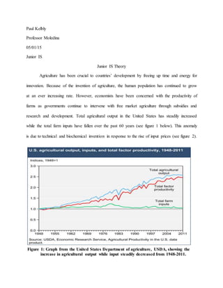
1. Paul Kelbly
Professor Moledina
05/01/15
Junior IS
Junior IS Theory
Agriculture has been crucial to countries’ development by freeing up time and energy for
innovation. Because of the invention of agriculture, the human population has continued to grow
at an ever increasing rate. However, economists have been concerned with the productivity of
farms as governments continue to intervene with free market agriculture through subsidies and
research and development. Total agricultural output in the United States has steadily increased
while the total farm inputs have fallen over the past 60 years (see figure 1 below). This anomaly
is due to technical and biochemical invention in response to the rise of input prices (see figure 2).
Figure 1: Graph from the United States Department of agriculture, USDA, showing the
increase in agricultural output while input steadily decreased from 1948-2011.

2. Kelbly 2
Figure 2: Shows the percentage of Private vs Public spending on agricultural R&D in
2007. Private spending makes up 53% of total expenditures on agricultural R&D.
In this paper, the author will look at the effects of government research and development
and policies on livestock productivity in the United States. In section I, the author will look at
how other economists have modeled and measured agricultural productivity. Then, he will setup
the theory of induced innovation to derive hypothesized results. In section III, the author will
draw conclusions from the theory of induced innovation.
I. Previous Work
Many economists have studied agricultural productivity, but few have looked at
agricultural production on a microeconomic scale. Wallace E. Huffman and Robert E. Evenson
looked at agricultural production on a macro level using the Solow Growth Model (Huffman and
Evenson 1992). The Solow Growth Model uses two inputs of labor, L, and capital, K, and
technology, A, to produce one output (see equation 1 below). The limitation of this model is that

3. Kelbly 3
it does not take into account the difference in individual markets. Many agricultural economists
generalize the whole market of agriculture and do not take into effect the differences between
individual farms in the livestock and crop sectors. Huffman and Evenson tried to mitigate this by
using the Solow Growth Model for each sector, livestock and crop (Huffman and Evenson 1992).
However, this still does not account for farms decisions based on changing prices of inputs.
Equation 1:
𝑌 = 𝐴𝐾∝
− 𝐿1−∝
One of the first agricultural economists to use a micro approach was Syed Ahmad
(Koppel 1995). He analyzed agricultural production through technical innovation using an
Innovation Possibilities Curve, IPC. The IPC is an envelope of different isoquant curves that
represent a given output using various production functions the entrepreneur plans to develop
(Koppel 1995). However, Ahmad’s theory assumes that new technologies are costless for
farmers to acquire. Private firms would invest in new technologies to save on a factor of
production, but Ahmad’s theory does not provide insight into public innovation.
Yujiro Hayami and Vernon Ruttan used Ahmad’s theory to develop their theory of
induced innovation (Koppel 1995). They introduced isocost curves into Ahmad’s IPC model to
analyze the effects on input prices on induced innovation. They split induced innovation into
technical and institutional change (Koppel 1995). Technical change is caused by a change in
the price of a factor of production and institutional change (Koppel 1995). Institutional change is
caused by a change in the price of a factor of production and technological change (Koppel
1995). This leads us to the current theory of induced innovation used to study agricultural
productivity on a micro scale.

4. Kelbly 4
II. The Theory of Induced Innovation
Before we study the theory of induced innovation, we must first understand isocost lines
and isoquant curves. The isocost line identifies all of the different combinations of inputs that
can be purchased given the Total Cost, TC. The slope of the isocost line equals the ratio of input
prices, −
𝑤
𝑟
; which is negative because the isocost line is downward sloping. W is the wages paid
for the input labor and r is the rent paid for the input capital.
𝑤
𝑟
is the rate at which one input can
be substituted for the other input (Browning 2012). Total Cost equals the price of labor, w, times
the quantity of labor employed, 𝑄𝐿, plus the price of capital, r, times the quantity of capital used,
𝑄 𝐾 (see equation 2 below). The isocost line moves northeast as the TC increases for the firm
allowing the firm to employ more inputs to produce more outputs. The total amount of labor that
can be hired equals TC/w and the total amount of capital that can be purchased equals TC/r.
Equation 2:
𝑇𝐶 = [( 𝑤 × 𝑄𝐿) + ( 𝑟 × 𝑄 𝐾)]
The isoquant curves are possible production functions the firm could have to reach a
certain output. The slope of the isoquant curve equals the Marginal Rate of Technical
Substitution, MRTS, which is the Marginal Product of Labor divided by the Marginal Product
Capital, 𝑀𝑃𝐿/𝑀𝑃𝐾. MRTS is the rate at which one input can be traded for the other input in
production (Browning 2012). When the isoquant curves move up and to the right, on the graph,
output increases (shown by the expansion path in figure 3). The tangency point on the graph is
the point at which the slope of the isocost line equals the slope of the isoquant curve, 𝑀𝑅𝑇𝑆 =
𝑤
𝑟
.
If we break this equation down we get
𝑀𝑃 𝐿
𝑀𝑃 𝐾
=
𝑤
𝑟
. Rearranging this equation we derive the new

5. Kelbly 5
equation: 𝑀𝑃𝐿/𝑤 = 𝑀𝑃 𝐾/𝑟 . This is the cost-minimization principle, which says that a firm should
employ its inputs in a way where the marginal product of labor per dollar spent on labor equals
the marginal product of capital per dollar spent on capital (Browning 2012). Minimizing costs
also means the farm wants to maximize profits by reducing costs.
Now that we understand the isocost lines and isoquant curves, we can develop the theory
of induced innovation. Induced innovation means that as the relative price of an input(s)
increases, the firm will invent new technologies to save or use less of that input(s) to reach a
certain output. The induced innovation theory is exactly the same as the isocost line and isoquant
Figure 3: Shows the expansion path of the tangency points and as isocost line moves
northeast total costs increase and as the isoquants move northeast output increases.

6. Kelbly 6
curve theory; however, the IPC from Ahmad’s IPC theory is introduced to show the various
isoquant curves the farm may operate under. The IPC is an envelope of different isoquant curves
that have various production functions to produce a given output. As the IPC shifts to the
northeast, output increases and vice versa. In the three scenarios to follow, the farm will try to
get back to the original IPC if a southwestern shift occurs, meaning output decreases, on the
graph. The price of both inputs may change simultaneously at the same rate or the price of a
single input may change where both situations cause the farm or the government to innovate to
save on that factor(s) of production and increase output.
The first scenario occurs when the price of capital and labor increase at the same rate.
Government R&D and policies will occur because an increase in the relative price of both inputs
causes the government to innovate through R&D and/or subsidies to save on those inputs called
the technical change effect (see equation 3 below). The increase in relative price for both inputs
will also cause the farmer to innovate to save on capital and labor. Increasing the relative price
of both inputs means that wage and the rent increase at the same rate. Graphically, this means
that the total cost will shift to the left to a new isocost line, B, isoquant curve, 𝐼𝑄𝐼
, and 𝐼𝑃𝐶 𝐼
(see
figure 4). Shifting to the left means that output will decrease, but through innovation, the r and w
will decrease brining output back to IPC.
Equation 3:
[( 𝑤 × 𝑄𝐿 ) + ( 𝑟 × 𝑄 𝐾 )] = 𝑇𝐶̅̅̅̅ = 𝐼𝑠𝑜𝑐𝑜𝑠𝑡 𝐿𝑖𝑛𝑒 𝐴
Where w and r increase at the same rate and then the quantity used of both inputs decreases and
TC is held constant.
[(↑ 𝑤 ×↓ 𝑄𝐿 ) + (↑ 𝑟 ×↓ 𝑄 𝐾 )] = 𝑇𝐶̅̅̅̅ = 𝐼𝑠𝑜𝑐𝑜𝑠𝑡 𝐿𝑖𝑛𝑒 𝐵
Innovation will occur to lower the price of w and r to get back to the output at IPC on isocost
line A.

7. Kelbly 7
This type of induced innovation occurred in China when the price of the staple crop, rice,
rose due to a shortage in 1960. The high price of rice caused the government to develop a high
yielding, stress resistant rice crop that allowed farmers to use fewer expensive inputs, such as
land and labor depending on the region, to increase rice production. At the same time, the
International Rice Research Institute, IRRI, developed a similar rice crop that allowed farmers to
produce rice using fewer inputs as well (Koppel 1995).
Figure 4: shows that as the price of capital and labor increase at the same rate, meaning the
slope does not change from isocost curve A to B, will lead a firm and/or the government to
innovate new ways to save on capital and labor that have become more expensive to use to get
back to the previous output of IPC.

8. Kelbly 8
The second scenario occurs when the price of a single input increases causing one of two
things to happen: 1) increase in the cost of one input moving the isocost line to the right or left
along the IPC because of the substitution effect or 2) an increase in the price of one input making
the isocost line pivot on the x-axis and move down along the y-axis. The effect of the first option
is caused by the increase in r lowering the quantity of capital used and lowering called the
substitution effect (shown by equation 3 and figure 5). In this case, the output stays the same by
using less of the expensive capital and more of the cheaper labor. Meaning, the isocost line stays
on the same IPC and no shift occurs. This means that the output will be the same after the price
of capital increases because the farm is on the same IPC curve by employing more labor and
using less capital. The farm would increase output if it moved to a different isoquant curve to the
northeast on the graph.
Equation 3:
[( 𝑤 × 𝑄𝐿 ) + ( 𝑃 𝑌 × 𝑄 𝑌)] = 𝑇𝐶 = 𝐼𝑠𝑜𝑐𝑜𝑠𝑡 𝐿𝑖𝑛𝑒 𝐴
Where r increases causing the firm to innovate for capital, saves on K, and use more labor in
production of that output.
[( 𝑤 ×↓ 𝑄𝐿 ) + ( 𝑟 ×↑ 𝑄 𝐾 )] = 𝑇𝐶 = 𝐼𝑠𝑜𝑐𝑜𝑠𝑡 𝐿𝑖𝑛𝑒 𝐵

9. Kelbly 9
The second option is that the isocost line will pivot on the x-axis from A to B causing the
farm to be on a new isoquant curve on the IPC to 𝐼𝑄𝐼
producing less output (see equation 4 and
figure 6). This occurs because the price increased for capital reducing the total amount of capital
that can be purchased and the price for labor stayed the same.
Equation 4:
[( 𝑤 × 𝑄𝐿 ) + ( 𝑟 × 𝑄 𝐾 )] = 𝑇𝐶 = 𝐼𝑠𝑜𝑐𝑜𝑠𝑡 𝐿𝑖𝑛𝑒 𝐴
Where r increases causing the farm to use less capital and less labor, but through innovation of
capital, the farm can use more capital to shift back to IPC to produce same output as before.
[( 𝑤 ×↓ 𝑄𝐿 ) + ( 𝑟 ×↓ 𝑄 𝐾 )] = 𝑇𝐶 = 𝐼𝑠𝑜𝑐𝑜𝑠𝑡 𝐿𝑖𝑛𝑒 𝐵
Figure 5: shows that as the price of capital rises, the farm will choose to use more labor and less of
capital. The rise in the price of capital causes farmers to innovate to save on that factor of production
to stay on the same IPC having the same output as before.

10. Kelbly 10
Ruttan and Hayami used this theory to describe the differences in Japan and the United
States’ agriculture from 1880-1890. They compared the inputs of farm draft horse power per
worker and fertilizer per hectare of agricultural land. Ruttan and Hayami saw that as the price of
fertilizer increased, the United States’ agriculture responded by having more equipment, draft
horse power per worker, to reduce the amount of fertilizer used to produce crops (Koppel 1995).
However, in Japan, the price for farm draft power per worker was very costly; therefore, Japan
used more fertilizer, which was cheaper than acquiring more horsepower. This means that farms
Figure 5: shows as the price of capital increases the total amount of capital used will decrease.
Therefore, less capital and labor will be used causing the farm to innovate to save on capital to
shift back to IPC on isocost line A.

11. Kelbly 11
in the United States chose to use technical innovation to increase horsepower per worker and
Japan chose to use institutional innovation by developing new types of fertilizers (Koppel 1995).
III. Induced Innovation in the Production Function
In the first scenario, we saw that the price of labor and the price of capital increased at the
same rate causing the farm to innovate. Innovation allowed the farm to use fewer amounts of
labor and capital to produce the same or more output than before. This is known as increasing
returns to scale when a firm has higher output relative to the inputs the firm used to produce
that output or the marginal product increases from the last marginal product. If you look at this
phenomenon graphically, the total product will be increasing, but will have a backward bend
because the farm is using fewer inputs to produce more output (shown in figure 7 below).
Figure 7: The production function is backward bending due to innovation
allowing the farm to use less capital to produce a higher output. This graph
represents the substitution effect the author graphed earlier in figure 5.

12. Kelbly 12
Figure 7 shows the production outcome that is occurring because of innovation. Point 𝑄1
corresponds to points 𝑄 𝐾
𝐼
in figures 5. The slope of the Total Product Line, also known as output,
at each point is equal to the Marginal Product of Capital. This graph is a simple representation of
how one factor affects production. The next step is to add in land and labor giving the graph two
more horizontal axes. This would allow us to see the points at which induced innovation
occurred, wherever the backward bend lies, and go beyond the two variable isoquant-isocost
graphs. In a typical isoquant-isocost graph, a shift to the southwest of the isoquant curve
indicates lower output; however, with induce innovation theory, a shift southwest indicates that
the farmer or the government will innovate new technologies to reach the same or higher outputs
when the isoquant shifts southwest.
IV. Conclusion and Limitations
According to the theory of induced innovation, if the prices of both capital and labor
increase simultaneously or as the price of one input increases, the government will innovate
through R&D or government subsidies. This allows for farms to use less of the expensive
input(s) to produce the same amount or more of the output as before the price increased for an
input(s).
The next step the author needs to take with his theory is to determine the lag-time it takes
for innovations to take full effect, the costs of R&D to the farm and the government, and develop
a production function and induced innovations graph containing land, labor, and capital. Lag-
time for R&D to have full effect on production and length of time the innovations have effects
on production is very difficult to understand. Lag-time is hard to determine because the observer
does not know the exact impact the new innovations are having on production or if something

13. Kelbly 13
else is affecting production. Also, there have been many empirical studies who account for lag-
time of innovation, but the authors estimates have varied greatly. Some authors have said the
average lag-time is 30-40 years, others said it is only 6-14 years, and some authors even predict a
lag-time of 50 years. The variable of time is tricky because of the difficulty measuring its effect
and knowing when and how long the lag-time affects production. Second, the author needs to
understand the costs of R&D to the farm and the government. New innovations are expensive to
develop causing many farmers to use technologies that have been created by other farmers or
governments. However, public extensions, such as land grant universities and USDA agencies,
will take on many costs to develop new technologies because individual farms do not want to
take on these costs. Currently, the most R&D comes from large private companies such as
Monsanto, Tyson, and Cargill. They develop new crops, breeds of animals, pesticides, and
herbicides that have caused production to increase steadily over the years with fewer inputs. The
costs associated with R&D are high and the author needs to fully understand the reasons why
governments and firms take on such high costs even if the benefit may be minimal. Lastly, the
author needs to develop his Induced Innovations Theory by including more inputs in his model.
This would help him understand each variable’s impact on one another, production and
understand why innovation occurs (see figures 8 and 9). The author needs to develop his theory
more by including lag-time, R&D costs, and multiple variables. These will help him understand
when R&D and policies take effect and for how long, reasons why governments and firms take
on risky endeavors, and the effects different variables have on productivity.

14. Kelbly 14
Figure 8: Initially the farm is at isocost line A on isoquant curve 1. Then the price of labor
increases moving the farm to isocost line B and isoquant curve 2. Therefore, the farm uses less
labor and substitutes more land for labor. As labor decreases and land use increase, the amount
of capital will increase as well from 𝑲 𝟏 to 𝑲 𝟐. The use of more capital in response to the increase
in the use of land is due to the buying of more equipment and other technologies in place of
labor. Output stays the same in this case and innovation occurs so the farm can use less labor and
more land and capital (Hockmann and Kopsidis 2007).

15. Kelbly 15
Figure 9: This is a model of the production function using capital and labor. If the author adds
land into this graph he would get another dimension to show the total output produced.

16. Kelbly 16
References
Browning, Edgar K. 2012. Microeconomics: Theory & Applications. 101h ed. Hoboken, NJ:
Wiley.
Hockmann, Heinrich, and Michael Kopsidis. 2007. “What Kind of Technological Change for
Russian Agriculture? The Transition Crisis of 1991–2005 from the Induced Innovation
Theory Perspective.” Post-Communist Economies 19 (1): 35–52.
doi:10.1080/14631370601163137.
Huffman, Wallace E., and Robert E. Evenson. 1992. “Contributions of Public and Private
Science and Technology to U.S. Agricultural Productivity.” American Journal of
Agricultural Economics 74 (3): 751–56.
Koppel, Bruce. 1995. Induced Innovation Theory and International Agricultural Development: A
Reassessment. Baltimore: Johns Hopkins University Press.