
Empfohlen
Empfohlen
Weitere ähnliche Inhalte
Was ist angesagt?
Was ist angesagt? (20)
Ähnlich wie Lecture 4 neural networks
Ähnlich wie Lecture 4 neural networks (20)
Mehr von ParveenMalik18
Kürzlich hochgeladen
Kürzlich hochgeladen (20)
Lecture 4 neural networks
- 1. Parveen Malik Assistant Professor KIIT University Neural Networks
- 2. Text Books: • Neural Networks and Learning Machines – Simon Haykin • Principles of Soft Computing- S.N.Shivnandam & S.N.Deepa • Neural Networks using Matlab- S.N. Shivanandam, S. Sumathi ,S N Deepa
- 3. What is Neural Network ?
- 4. “A neural network is a massively parallel distributed processor made up of simple processing units that has a natural propensity for storing experiential knowledge and making it available for use.” It resembles the brain in two respects: 1. Knowledge is acquired by the network from its environment through a learning process. 2. Interneuron connection strengths, known as synaptic weights, are used to store the acquired knowledge. Neural Network
- 5. Why we need Neural Networks ?
- 6. Object Detection Visual Tracking Image Captioning Video Captioning Visual Question Answering Video question answering Video Summarization Generating Authentic Photos Facial Expression detection Machine Learning Visual Pattern Recognition Natural Language Processing Language Modelling Text prediction Speech Recognition Machine Translation C-H conversation Modelling Time series Modelling Share Market Prediction Weather Forecasting Financial Data analytics Mood analytics Machine Learning and Beyond
- 8. Aerospace Defence High performance aircraft autopilot Flight path simulations Aircraft control system Autopilot enhancements Aircraft component simulations Aircraft component detectors. Weapon steering Target tracking Object discrimination Facial recognition New kind of sensors Sonar Radar signal processing image signal processing Data compression Feature extraction Noise suppression Manufacturing Manufacturing process control Product design and analysis Process and machine diagnosis Real time particle identification Visual quality inspection systems Wielding analysis Analysis of grinding operations Chemical product design, analysis Machine maintenance analysis Project bidding planning and management Dynamic modelling of chemical process systems. Medical Entertainment Breast cancer cell analysis EEG and ECG analysis Prosthesis design Optimization of transplant times Hospital expense reduction Hospital quality improvement Emergency room test advisement Animation Special effects Market forecasting Electronics Code sequence prediction Integrated circuit chip layout Process control Chip failure analysis Machine vision Voice synthesis Non-linear modelling Applications
- 9. Financial Telecommunications • Real estate appraisal • Loan advisor • Mortgage screening • Corporate bond rating • Credit line use analysis • Portfolio trading program • Corporate financial analysis • Currency price prediction • Image and data compression • Automated information services • Real time translation of spoken language • Customer payment processing systems Securities • Market analysis • Automatic bond rating • Stock trading advisory systems Automotive Banking • Automobile automatic guidance systems • Warranty activity analysers • Check and other document readers • Credit application evaluators Insurance Policy application evaluation Product optimization Robotics • Trajectory control • Forklift robot • Manipulator controllers • Vision systems Speech Transportation • Speech recognition • Speech compression • Vowel classification • Text to speech synthesis • Truck brake diagnosis systems • Vehicle scheduling • Routing systems
- 10. Central Nervous System Human Brain and Neuron
- 11. CNS- Brain and Neuron Neuron - Structural Unit of central nervous system i.e. Brain and Spinal Cord. • 100 billion neurons, 100 trillion synapses • Weight -1.5 Kg to 2Kg • Conduction Speed – 0.6 m/s to 120 m/s • Power – 20% ,20-40 Watt,10−16 𝐽 𝑜𝑝𝑒𝑟𝑎𝑡𝑖𝑜𝑛𝑠 • Ion Transport Phenomenon • Fault tolerant • Asynchronous firing • Response time = 10−3 sec “The Brain is a highly complex, non-linear and massively parallel Computing machine.” 𝑵𝒆𝒖𝒓𝒐𝒏
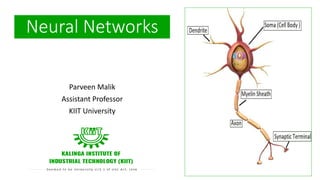
- 12. “A Neuron is a basic unit of brain that processes and transmits information.” Neuron • Dendrite: Receive signals from other neurons • Soma (Cell body): Process the incoming signals. • Myelin Sheath: Covers neurons and help speed up neuron impulses. • Axon : Transmits the electric potential from soma to synaptic terminal and then finally to other neurons, muscles or glands • Synaptic Terminal : Release the neurotransmitter to transmit information to dendrites.
- 14. Hierarchal Learning – Inspired Deep Learning Human Brain Contd.
- 15. Historical Perspective about modelling of Brain through Medical and Applied Mathematics World
- 19. Analogy between Biological Neural Network and Artificial Neural Network
- 20. Biological Neural Network Vs Artificial Neural Network Equivalent Electrical Model
- 21. Practical Neural Network (Single Neuron) 𝑥1 𝑥2 𝑥𝑛 ⋮ 𝑤1 𝑤2 𝑤𝑛 ෝ 𝒚 = 𝒇 𝒊=𝟏 𝒏 𝒘𝒊𝒙𝒊 + 𝒃 (𝐢𝐧𝐩𝐮𝐭) 𝑓 Actual Output Inputs b (Bias) 𝑥1 𝑥2 𝑥𝑛 ⋮ 𝑤1 𝑤2 𝑤𝑛 ෝ 𝒚 = 𝒇 𝒊=𝟎 𝒏 𝒘𝒊𝒙𝒊 (𝐢𝐧𝐩𝐮𝐭) 𝑓 Actual Output (Bias) 𝑤0=b 𝑥0 = 1 Bias is 0th weight with input equal to 1
- 22. Activation Functions Name Geometrical Shape Mathematical Expression Property Hard Limit 𝒇 𝒙 = ቊ 𝟏 𝒊𝒇 𝒙 ≥ 𝟎 𝟎 𝒐𝒕𝒉𝒆𝒓𝒘𝒊𝒔𝒆 Non-differentiable Bipolar Hard Limit Signum Function 𝒇 𝒙 = ቐ 𝟏 𝟎 −𝟏 𝒊𝒇 𝒙 > 𝟎 𝒊𝒇 𝒙 = 𝟎 𝒊𝒇 𝒙 < 𝟎 Non-differentiable Sigmoid Function 𝒇 𝒙 = 𝟏 𝟏 + 𝒆−𝒙 Differentiable 𝒇′ 𝒙 = 𝒇 𝒙 𝟏 − 𝒇 𝒙 1 0 𝒙 𝒇 𝒙 1 0 𝒙 𝒇 𝒙 -1 1 0 𝒇 𝒙
- 23. Activation Functions Name Geometrical Shape Mathematical Expression Property Hyperbolic Tangent or Bipolar sigmoid 𝒇 𝒙 = 𝒕𝒂𝒏𝒉𝒙 = 𝒆𝒙−𝒆−𝒙 𝒆𝒙+𝒆−𝒙 Differentiable 𝒇′ 𝒙 = 𝟏 − 𝒇𝟐 𝒙 Bipolar Hard Limit Signum Function 𝒇 𝒙 = 𝒙 Differentiable Rectified Linear Unit 𝒇 𝒙 = 𝒎𝒂𝒙(𝟎, 𝒙) Differentiable 0 1 0 𝒙 𝒇 𝒙 -1 𝒇 𝒙 𝒙 𝒇 𝒙 𝒙 0
- 24. Single Perceptron to Multiple layer of perceptron – Historical Perspective McCulloch Pitts (1943) – 1st Mathematical model of neuron Weighted sum of input signals is compared to a threshold to determine the neuron output Hebbian Learning Algorithm -1949 Learning of weights to classify the patterns Organization of Behaviour – David Hebb Frank Rosenblatt (1957) – More Accurate Neuron Model (Perceptron) Perceptron Learning Algorithm to find optimum weights Perceptron Learning Algorithm Delta rule or Widrow- Hoff Learning Algorithm Approximate steepest descent algorithm Least Means Square Algorithm Adaptive Linear Neuron Network Learning Marvin Minsky and Seymour Peppert (1969) Limitation of perceptron in classifying Non separable Patterns Back Propagation (1986) Training of Multilayer of Perceptrons 𝑾𝒏𝒆𝒘 = 𝑾𝒐𝒍𝒅 + 𝒙𝒊𝒚 𝑾𝒏𝒆𝒘 = 𝑾𝒐𝒍𝒅 + (𝒕 − 𝒂)𝒙𝒊 𝑾𝒏𝒆𝒘 = 𝑾𝒐𝒍𝒅 − ቚ 𝜶𝛁𝑭 𝒘 𝒘=𝑾𝒐𝒍𝒅
- 25. Geometrical Significance (Hardlimit activation function) 𝑥1 𝑥2 𝑥𝑛 ⋮ 𝑤1 𝑤2 𝑤𝑛 ෝ 𝒚 = 𝒇 𝒊=𝟏 𝒏 𝒘𝒊𝒙𝒊 + 𝒃 (𝐢𝐧𝐩𝐮𝐭) 𝑓 Inputs b (Bias) Hyperplane Activation Function 0 1 Output input Hard limit Function From Activation function, we can infer if σ𝒊=𝟏 𝒏 𝒘𝒊𝒙𝒊 + 𝒃 or 𝑾𝑻 𝑿 (inner product between weight vector and input vector) is greater than 0 for output is 1. 𝐰𝐡𝐞𝐫𝐞, 𝐰𝐞𝐢𝐠𝐡𝐭 𝐯𝐞𝐜𝐭𝐨𝐫 , 𝐖 = 𝐰𝟏 𝐰𝟐 ⋮ 𝐰𝐧 and input vector, 𝑿 = 𝒙𝟏 𝒙𝟐 ⋮ 𝒙𝒏 . The σ𝒊=𝟏 𝒏 𝒘𝒊𝒙𝒊 + 𝒃 = 𝟎 is equivalent to a hyperplane boundary.
- 26. Geometrical Significance (Hardlimit Activation function) 2 input (𝒙𝟏 & 𝒙𝟐) → Boundary is line (𝒘𝟏𝒙𝟏 + 𝒘𝟐𝒙𝟐+b=0) with 𝒘𝟏, 𝒘𝟐 𝒂𝒔 𝒏𝒐𝒓𝒎𝒂𝒍 ⊥ 𝒗𝒆𝒄𝒕𝒐𝒓 𝒐𝒇 𝒍𝒊𝒏𝒆 . 3 input (𝒙𝟏, 𝒙𝟐 & 𝒙𝟑) → Boundary is Plane (𝒘𝟏𝒙𝟏 + 𝒘𝟐𝒙𝟐+𝒘𝟑𝒙𝟑+b=0) with 𝒘𝟏, 𝒘𝟐, 𝒘𝟑 𝒂𝒔 𝒏𝒐𝒓𝒎𝒂𝒍 ⊥ 𝒗𝒆𝒄𝒕𝒐𝒓 𝒐𝒇 𝒑𝒍𝒂𝒏𝒆. >3 input (𝒙𝟏, 𝒙𝟐,⋯ 𝒙𝒏) → Boundary is Hyperplane (𝒘𝟏𝒙𝟏 + 𝒘𝟐𝒙𝟐+⋯+𝒘𝒏𝒙𝒏+b=0) with 𝒘𝟏, 𝒘𝟐 ⋯ 𝒘𝒏 𝒂𝒔 𝒏𝒐𝒓𝒎𝒂𝒍 ⊥ 𝒗𝒆𝒄𝒕𝒐𝒓 𝒐𝒇 𝒉𝒚𝒑𝒆𝒓𝒑𝒍𝒂𝒏𝒆. 𝐖𝐞𝐢𝐠𝐡𝐭 𝐕𝐞𝐜𝐭𝐨𝐫 (𝐰𝟏, 𝐰𝟐) 𝑳𝒊𝒏𝒆 𝑬𝒒𝒖𝒂𝒕𝒊𝒐𝒏 (𝐰𝟏𝐱𝟏 + 𝐱𝟐𝐰𝟐+b=0) Class 1 Class 2 𝐖𝐞𝐢𝐠𝐡𝐭 𝐕𝐞𝐜𝐭𝐨𝐫 (𝐰𝟏, 𝐰𝟐, 𝐰𝟑) 𝑷𝒍𝒂𝒏𝒆 𝑬𝒒𝒖𝒂𝒕𝒊𝒐𝒏 (𝐰𝟏𝐱𝟏 + 𝐱𝟐𝐰𝟐++𝐱𝟑𝐰𝟑+b=0) Class 1 Class 2 𝐱𝟏 𝐱𝟐 𝐱𝟏 𝐱𝟐 𝐱𝟑 2 Class Single Neuron Classification
- 28. McCulloch Pitts Neuron (1943) Mathematical Model of the brain Depends upon the threshold (𝜃) with a hard limit activation function 𝒚𝒊𝒏 𝑓 𝒚𝒊𝒏 𝑦 = 𝑓 𝒚𝒊𝒏 𝑥1 𝑥2 𝑥𝑛 ⋮ 𝑤2 𝑤1 𝑤𝑛 𝑓 𝒚𝒊𝒏 = ቊ 𝟏 if 𝒚𝒊𝒏 ≥ 𝜽 𝟎 𝒐𝒕𝒉𝒆𝒓𝒘𝒊𝒔𝒆 𝜽 OR Gate 𝒙𝟏 𝒙𝟐 Target Output (𝒚) 0 0 0 0 1 1 1 0 1 1 1 1 𝒚𝒊𝒏 𝑓 𝒚𝒊𝒏 𝑦 = 𝑓 𝒚𝒊𝒏 𝑥1 𝑥2 𝑤1 = 1 𝑤2=1 𝑓 𝒚𝒊𝒏 = ቊ 𝟏 if 𝒚𝒊𝒏 ≥ 𝟏 𝟎 𝒐𝒕𝒉𝒆𝒓𝒘𝒊𝒔𝒆 𝜽 = 𝟏 𝒚𝒊𝒏= 𝒘𝟏𝒙𝟏 + 𝒘𝟐𝒙𝟐 = 𝒙𝟏 + 𝒙𝟐
- 29. McCulloch Pitts Neuron AND Gate 𝒙𝟏 𝒙𝟐 Target Output (𝒚) 0 0 0 0 1 0 1 0 0 1 1 1 𝒚𝒊𝒏 𝑓 𝒚𝒊𝒏 𝑦 = 𝑓 𝒚𝒊𝒏 𝑥1 𝑥2 𝑤1 = 1 𝑤2=1 𝑓 𝒚𝒊𝒏 = ቊ 𝟏 if 𝒚𝒊𝒏 ≥ 𝟐 𝟎 𝒐𝒕𝒉𝒆𝒓𝒘𝒊𝒔𝒆 𝜽 = 𝟐 𝒚𝒊𝒏= 𝒘𝟏𝒙𝟏 + 𝒘𝟐𝒙𝟐 = 𝒙𝟏 + 𝒙𝟐 Not Gate 𝑥 Target Output (𝒚) 0 1 1 0 𝒚𝒊𝒏 𝑓 𝒚𝒊𝒏 𝑦 = 𝑓 𝒚𝒊𝒏 𝑥 𝑤1 = 1 𝑓 𝒚𝒊𝒏 = ቊ 𝟏 if 𝒚𝒊𝒏 < 𝟎 𝟎 if 𝒚𝒊𝒏 ≥ 𝟏 𝒚𝒊𝒏= 𝒘𝟏𝒙 = 𝒙
- 30. McCulloch Pitts Neuron (XOR implementation) 𝒙𝟏 𝒙𝟐 Target Output (𝒚=𝒙𝟏 𝑻 𝒙𝟐) 0 0 0 0 1 1 1 0 0 1 1 0 𝒚𝒊𝒏 𝑓 𝒚𝒊𝒏 𝑦 = 𝑓 𝒚𝒊𝒏 𝑥1 𝑥2 𝒘𝟏 = −𝟏 𝒘𝟐= 1 𝑓 𝒚𝒊𝒏 = ቊ 𝟏 if 𝒚𝒊𝒏 ≤ −𝟏 𝟎 𝒐𝒕𝒉𝒆𝒓𝒘𝒊𝒔𝒆 𝜽 = −𝟏 𝒚𝒊𝒏= 𝒘𝟏𝒙𝟏 + 𝒘𝟐𝒙𝟐 = 𝒙𝟐 − 𝒙𝟏 𝒙𝟏 𝒙𝟐 Target Output (𝒚=𝒙𝟏𝒙𝟐 𝑻 ) 0 0 0 0 1 0 1 0 1 1 1 0 𝒚𝒊𝒏 𝑓 𝒚𝒊𝒏 𝑦 = 𝑓 𝒚𝒊𝒏 𝑥1 𝑥2 𝒘𝟏 = 𝟏 𝒘𝟐=-1 𝑓 𝒚𝒊𝒏 = ቊ 𝟏 if 𝒚𝒊𝒏 ≤ −𝟏 𝟎 𝒐𝒕𝒉𝒆𝒓𝒘𝒊𝒔𝒆 𝜽 = −𝟏 𝒚𝒊𝒏= 𝒘𝟏𝒙𝟏 + 𝒘𝟐𝒙𝟐 = 𝒙𝟏 − 𝒙𝟐 𝒚=𝒙𝟏 𝑻 𝒙𝟐 𝒚=𝒙𝟏𝒙𝟐 𝑻
- 31. McCulloch Pitts Neuron (XOR implementation- 3 Neurons) 𝒙𝟏 𝒙𝟐 𝒚𝟏=𝒙𝟏 𝑻 𝒙𝟐 𝒚𝟐=𝒙𝟏𝒙𝟐 𝑻 𝒚=𝒙𝟏 𝑻 𝒙𝟐 + 𝒙𝟏𝒙𝟐 𝑻 0 0 0 0 0 0 1 1 0 1 1 0 0 1 1 1 1 0 0 0 𝒚=𝒙𝟏 𝑻 𝒙𝟐 + 𝒙𝟏𝒙𝟐 𝑻 𝒚𝒊𝒏𝟏= 𝒘𝟏𝒙𝟏 + 𝒘𝟐𝒙𝟐 = 𝒙𝟏 − 𝒙𝟐 𝑦 = 𝑓 𝒚𝒊𝒏 𝒙𝟏 𝒙𝟐 𝒚𝒊𝒏𝟏 𝑓 𝒚𝒊𝒏𝟏 𝒘𝟏𝟏 = 𝟏 𝒘𝟏𝟐 = −𝟏 𝒘𝟐𝟏 = −𝟏 𝒚𝒊𝒏 𝑓 𝒚𝒊𝒏 𝒚𝒊𝒏𝟐 𝑓 𝒚𝒊𝒏𝟐 𝒘𝟐𝟐 = 𝟏 𝒚𝒊𝒏𝟐= 𝒘𝟏𝒙𝟏 + 𝒘𝟐𝒙𝟐 = 𝒙𝟐 − 𝒙𝟏 𝒘𝟏𝟏 (𝟏) = 𝟏 𝒘𝟏𝟐 (𝟏) = 𝟏
- 33. Hebbian Learning Rule • Donald Hebb (Psychologist)– The Organization of the behaviour (1949) • Hebb’s Postulate – “When an axon of cell A is near enough to excite a cell B and repeatedly or persistently takes part in firing it, some growth process or metabolic change takes place in one or both cells such that A’s efficiency, as one of the cells firing B, is increased.” Mathematically, 𝑾𝒏𝒆𝒘= 𝑾𝒐𝒍𝒅 + 𝒙𝒊𝒚 Where 𝑥𝑖 is the ith input and 𝑦 is output. Bipolar inputs or outputs (-1 or +1) Limitation – Can classify linearly separable patterns only
- 34. Hebbian Learning Rule 𝑾𝑵𝒆𝒘 = 𝑾𝒐𝒍𝒅 + 𝒙𝒊𝒚 Bipolar inputs or outputs (-1 or +1) AND gate Implementation 𝒙𝟏 𝒙𝟐 Target Output (𝒚) ∆𝒘𝟏 ∆𝒘𝟐 ∆𝒃 𝒘𝟏 0 𝒘𝟐 0 𝒘𝟎(𝒃) 0 -1 -1 -1 1 1 -1 1 1 -1 -1 1 -1 1 -1 -1 2 0 -2 1 -1 -1 -1 1 -1 1 1 -3 1 1 1 1 1 1 2 2 -2 Initialized weight & bias 𝒘𝟏(𝒏𝒆𝒘) = 𝒘𝟏(𝒐𝒍𝒅) + 𝒙𝟏𝒚 𝒘𝟐(𝒏𝒆𝒘) = 𝒘𝟐(𝒐𝒍𝒅) + 𝒙𝟐𝒚 𝒘𝟎(𝒏𝒆𝒘) = 𝒘𝟎(𝒐𝒍𝒅) + 𝒙𝟎𝒚 (𝑭𝒐𝒓 𝒃𝒊𝒂𝒔 𝒙𝟎 = 𝟏 & 𝒘𝟎 = 𝒃) 𝒚𝒊𝒏= 𝒘𝟎𝒙𝟎 + 𝒘𝟏𝒙𝟏 + 𝒘𝟐𝒙𝟐 = 𝒃 + 𝒘𝟏𝒙𝟏 + 𝒘𝟐𝒙𝟐 𝒙𝟎 = 𝟏 𝒚𝒊𝒏 𝑓 𝒚𝒊𝒏 ෝ 𝒚 = 𝒇 𝒚𝒊𝒏 𝒙𝟐 𝒙𝟏 𝒘𝟏 𝒘𝟐 𝒘𝟎= b 1 epoch Iterations
- 35. Hebbian Learning Rule OR gate Implementation 𝒙𝟏 𝒙𝟐 Target Output (𝒚) ∆𝒘𝟏 ∆𝒘𝟐 ∆𝒃 𝒘𝟏 0 𝒘𝟐 0 𝒘𝟎(𝒃) 0 -1 -1 -1 1 1 -1 1 1 -1 -1 1 1 -1 1 1 0 2 0 1 -1 1 1 -1 1 1 1 1 1 1 1 1 1 1 2 2 2 Initialized weight & bias 1 epoch Iterations Check : 𝒚𝒊𝒏 𝑓 𝒚𝒊𝒏 ෝ 𝒚 = 𝒇 𝒚𝒊𝒏 Where, 𝒇 𝒚𝒊𝒏 = ቊ 𝟏, 𝒚𝒊𝒏 ≥ 𝟎 𝟎, 𝒚𝒊𝒏 < 𝟎 𝒙𝟐 𝒙𝟏 𝒘𝟏 = 𝟐 𝒘𝟐 = 𝟐 𝒘𝟎= 2 𝒙𝟎 = 𝟏 -1 -1 𝒚𝒊𝒏 = -2 𝒇(𝒚𝒊𝒏) = 𝒇(−𝟐)=0
- 36. Hebbian Learning Rule OR gate Implementation 𝒙𝟏 𝒙𝟐 Target Output (𝒚) ∆𝒘𝟏 ∆𝒘𝟐 ∆𝒃 𝒘𝟏 0 𝒘𝟐 0 𝒘𝟎(𝒃) 0 -1 -1 -1 1 1 -1 1 1 -1 -1 1 1 -1 1 1 0 2 0 1 -1 1 1 -1 1 1 1 1 1 1 1 1 1 1 2 2 2 Initialized weight & bias 1 epoch Iterations Check : 𝒚𝒊𝒏 𝑓 𝒚𝒊𝒏 ෝ 𝒚 = 𝒇 𝒚𝒊𝒏 Where, 𝒇 𝒚𝒊𝒏 = ቊ 𝟏, 𝒚𝒊𝒏 ≥ 𝟎 𝟎, 𝒚𝒊𝒏 < 𝟎 𝒙𝟐 𝒙𝟏 𝒘𝟏 = 𝟐 𝒘𝟐 = 𝟐 𝒘𝟎= 2 𝒙𝟎 = 𝟏 1 1 𝒚𝒊𝒏 = 6 𝒇(𝒚𝒊𝒏) = 𝒇 𝟔 = 1
- 37. Hebbian Learning Rule OR gate Implementation 𝒙𝟏 𝒙𝟐 Target Output (𝒚) ∆𝒘𝟏 ∆𝒘𝟐 ∆𝒃 𝒘𝟏 0 𝒘𝟐 0 𝒘𝟎(𝒃) 0 -1 -1 -1 1 1 -1 1 1 -1 -1 1 1 -1 1 1 0 2 0 1 -1 1 1 -1 1 1 1 1 1 1 1 1 1 1 2 2 2 Initialized weight & bias 1 epoch Iterations Check : 𝒚𝒊𝒏 𝑓 𝒚𝒊𝒏 ෝ 𝒚 = 𝒇 𝒚𝒊𝒏 Where, 𝒇 𝒚𝒊𝒏 = ቊ 𝟏, 𝒚𝒊𝒏 ≥ 𝟎 𝟎, 𝒚𝒊𝒏 < 𝟎 𝒙𝟐 𝒙𝟏 𝒘𝟏 = 𝟐 𝒘𝟐 = 𝟐 𝒘𝟎= 2 𝒙𝟎 = 𝟏 -1 1 𝒚𝒊𝒏= 2 𝒇(𝒚𝒊𝒏) = 𝒇(𝟐)=1 Q - Are these Optimum set of weights ?
- 39. Perceptron Learning Rule • Frank Rosenblatt – (1957) • Key contribution - Introduction of a learning rule for training perceptron networks to solve pattern recognition problems • Perceptron could even learn when initialized with random values for its weights and biases. • Limitations – Can classify only linearly separable problems. • Limitations were publicized in the book “Perceptrons (1969)” by Marvin Minsky and Seymour Peppert. Mathematically, 𝑾𝒏𝒆𝒘= 𝑾𝒐𝒍𝒅 + (𝒚 − ෝ 𝒚) 𝒙𝒊 Where, 𝑥𝑖 𝑖𝑠 𝑖𝑡ℎ 𝑖𝑛𝑝𝑢𝑡, ො 𝑦 𝑖𝑠 𝑎𝑐𝑡𝑢𝑎𝑙 𝑜𝑟 𝑝𝑟𝑒𝑑𝑖𝑐𝑡𝑒𝑑 𝑜𝑢𝑡𝑝𝑢𝑡 𝑎𝑛𝑑 𝑦 𝑖𝑠 𝑡𝑎𝑟𝑔𝑒𝑡 𝑜𝑢𝑡𝑝𝑢𝑡.
- 40. Perceptron Learning Rule 𝑾𝑵𝒆𝒘 = 𝑾𝒐𝒍𝒅 + (𝒚 − ෝ 𝒚)𝒙𝒊 AND gate Implementation 𝒙𝟏 𝒙𝟐 Target Output (𝒚) Actual Output (ෝ 𝒚) (𝒚 − ෝ 𝒚) ∆𝒘𝟏 =(𝒚 − ෝ 𝒚)𝒙𝟏 ∆𝒘𝟐 = (𝒚 − ෝ 𝒚)𝒙𝟐 ∆𝒃 = (𝒚 − ෝ 𝒚) 𝒘𝟏 0 𝒘𝟐 0 𝒘𝟎(𝒃) 0 0 0 0 1 -1 0 0 -1 0 0 -1 0 1 0 0 0 0 0 0 0 0 -1 1 0 0 0 0 0 0 0 0 0 -1 1 1 1 0 1 1 1 1 1 1 0 Initialized weight & bias 𝒘𝟏(𝒏𝒆𝒘) = 𝒘𝟏(𝒐𝒍𝒅) + ∆𝒘𝟏 = 𝒘𝟏(𝒐𝒍𝒅) +(𝒚 − ෝ 𝒚)𝒙𝟏 𝒘𝟐(𝒏𝒆𝒘) = 𝒘𝟐(𝒐𝒍𝒅) + ∆𝒘𝟐 = 𝒘𝟐(𝒐𝒍𝒅) +(𝒚 − ෝ 𝒚)𝒙𝟐 𝒘𝟎(𝒏𝒆𝒘) = 𝒘𝟎(𝒐𝒍𝒅) +(𝒚 − ෝ 𝒚)𝒙𝟎 (𝑭𝒐𝒓 𝒃𝒊𝒂𝒔 𝒙𝟎 = 𝟏 & 𝒘𝟎 = 𝒃) 𝒚𝒊𝒏= 𝒘𝟎𝒙𝟎 + 𝒘𝟏𝒙𝟏 + 𝒘𝟐𝒙𝟐 = 𝒃 + 𝒘𝟏𝒙𝟏 + 𝒘𝟐𝒙𝟐 𝒙𝟎 = 𝟏 𝒚𝒊𝒏 𝑓 𝒚𝒊𝒏 ෝ 𝒚 = 𝒇 𝒚𝒊𝒏 𝒇 𝒚𝒊𝒏 = ቊ 𝟏, 𝒚𝒊𝒏 ≥ 𝟎 𝟎, 𝒚𝒊𝒏 < 𝟎 𝒙𝟐 𝒙𝟏 𝒘𝟏 𝒘𝟐 𝒘𝟎= b 1 epoch Iterations Weights after 1 epoch
- 41. OR gate Implementation Initialized weight & bias 1 epoch Iterations Check : 𝒚𝒊𝒏 𝑓 𝒚𝒊𝒏 ෝ 𝒚 = 𝒇 𝒚𝒊𝒏 Where, 𝒇 𝒚𝒊𝒏 = ቊ 𝟏, 𝒚𝒊𝒏 ≥ 𝟎 𝟎, 𝒚𝒊𝒏 < 𝟎 𝒙𝟐 𝒙𝟏 𝒘𝟏 = 𝟏 𝒘𝟐 = 𝟎 𝒘𝟎= 0 𝒙𝟎 = 𝟏 0 0 𝒚𝒊𝒏 = 0 𝒇(𝒚𝒊𝒏) = 𝒇 𝟎 = 1 𝒙𝟏 𝒙𝟐 Target Output (𝒚) Actual Output (ෝ 𝒚) (𝒚 − ෝ 𝒚) ∆𝒘𝟏 =(𝒚 − ෝ 𝒚)𝒙𝟏 ∆𝒘𝟐 = (𝒚 − ෝ 𝒚)𝒙𝟐 ∆𝒃 = (𝒚 − ෝ 𝒚) 𝒘𝟏 0 𝒘𝟐 0 𝒘𝟎(𝒃) 0 0 0 0 1 -1 0 0 -1 0 0 -1 0 1 1 0 1 0 1 1 0 1 0 1 0 1 1 0 0 0 0 0 1 0 1 1 1 1 0 0 0 0 0 1 0 × 𝑾𝒓𝒐𝒏𝒈 Output Need more iterations Perceptron Learning Rule