Copy Of Consumer
•Download as XLS, PDF•
0 likes•308 views

Statistical Analysis Regression Multiple. Excel Capability

Recommended
More Related Content
What's hot
Viewers also liked
Viewers also liked (20)
Similar to Copy Of Consumer
Similar to Copy Of Consumer (20)
Copy Of Consumer
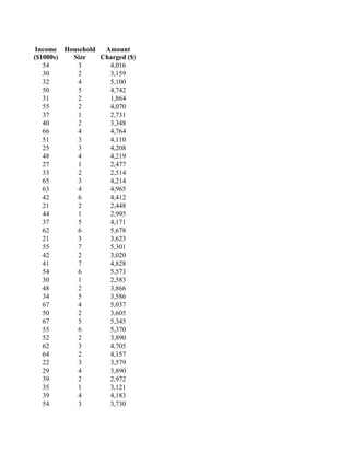
- 1. Income Household Amount ($1000s) Size Charged ($) 54 3 4,016 30 2 3,159 32 4 5,100 50 5 4,742 31 2 1,864 55 2 4,070 37 1 2,731 40 2 3,348 66 4 4,764 51 3 4,110 25 3 4,208 48 4 4,219 27 1 2,477 33 2 2,514 65 3 4,214 63 4 4,965 42 6 4,412 21 2 2,448 44 1 2,995 37 5 4,171 62 6 5,678 21 3 3,623 55 7 5,301 42 2 3,020 41 7 4,828 54 6 5,573 30 1 2,583 48 2 3,866 34 5 3,586 67 4 5,037 50 2 3,605 67 5 5,345 55 6 5,370 52 2 3,890 62 3 4,705 64 2 4,157 22 3 3,579 29 4 3,890 39 2 2,972 35 1 3,121 39 4 4,183 54 3 3,730
- 2. 23 6 4,127 27 2 2,921 26 7 4,603 61 2 4,273 30 2 3,067 22 4 3,074 46 5 4,820 66 4 5,149
- 3. Income Household ($1000s) Size Mean 43.48 Mean 3.42 Standard Error 2.06 Standard Error 0.25 Median 42 Median 3 Mode 54 Mode 2 Standard Deviation 14.55 Standard Deviation 1.74 Sample Variance 211.72 Sample Variance 3.02 Kurtosis -1.25 Kurtosis -0.72 Skewness 0.1 Skewness 0.53 Range 46 Range 6 Minimum 21 Minimum 1 Maximum 67 Maximum 7 Sum 2174 Sum 171 Count 50 Count 50 Confidence Level(95.0%) 4.14 Confidence Level(95.0%) 0.49
- 4. Amount Charged ($) Mean 3964.06 Standard Error 132.02 Median 4090 Mode 3890 Standard Deviation 933.49 Sample Variance 871411.2 Kurtosis -0.74 Skewness -0.13 Range 3814 Minimum 1864 Maximum 5678 Sum 198203 Count 50 Confidence Level(95.0%) 265.3
- 5. SUMMARY OUTPUT Regression Statistics Multiple R 0.63 R Square 0.4 Adjusted R Square 0.39 Standard Error 731.71 Observations 50 ANOVA df SS MS F Significance F Regression Residual 1 48 ### ### ### 535404.25 31.75 0 ($1000 Total 49 ### 6000 Charged ($) Coefficients Standard Error t Stat P-value Lower 95% Upper 95% 4000 Amount Intercept 2204 329.05 6.7 0 1542.4 2865.6 Income ($1000s) 40.48 7.18 5.63 0 26.04 54.92 2000 RESIDUAL OUTPUT 0 PROBABILITY OUTPUT Predicted 10 20 30 Amount Amount Charged Charged Inco Observation ($) Residuals Standard Residuals Percentile ($) 1 4389.91 -373.91 -0.52 1 1864 ($10 2 3418.39 -259.39 -0.36 3 2448 3 3499.35 1600.65 2.21 5 2477 4 4227.99 514.01 0.71 7 2514 5 3458.87 -1594.87 -2.2 9 2583 6 4430.39 -360.39 -0.5 11 2731 7 3701.75 -970.75 -1.34 13 2921 8 3823.19 -475.19 -0.66 15 2972 9 4875.66 -111.66 -0.15 17 2995 10 4268.47 -158.47 -0.22 19 3020 11 3215.99 992.01 1.37 21 3067 12 4147.03 71.97 0.1 23 3074 13 3296.95 -819.95 -1.13 25 3121 14 3539.83 -1025.83 -1.42 27 3159 15 4835.18 -621.18 -0.86 29 3348 16 4754.23 210.77 0.29 31 3579 17 3904.15 507.85 0.7 33 3586
- 6. 18 3054.07 -606.07 -0.84 35 3605 19 3985.11 -990.11 -1.37 37 3623 20 3701.75 469.25 0.65 39 3730 21 4713.75 964.25 1.33 41 3866 22 3054.07 568.93 0.79 43 3890 23 4430.39 870.61 1.2 45 3890 24 3904.15 -884.15 -1.22 47 4016 25 3863.67 964.33 1.33 49 4070 26 4389.91 1183.09 1.63 51 4110 27 3418.39 -835.39 -1.15 53 4127 28 4147.03 -281.03 -0.39 55 4157 29 3580.31 5.69 0.01 57 4171 30 4916.14 120.86 0.17 59 4183 31 4227.99 -622.99 -0.86 61 4208 32 4916.14 428.86 0.59 63 4214 33 4430.39 939.61 1.3 65 4219 34 4308.95 -418.95 -0.58 67 4273 35 4713.75 -8.75 -0.01 69 4412 36 4794.7 -637.7 -0.88 71 4603 37 3094.55 484.45 0.67 73 4705 38 3377.91 512.09 0.71 75 4742 39 3782.71 -810.71 -1.12 77 4764 40 3620.79 -499.79 -0.69 79 4820 41 3782.71 400.29 0.55 81 4828 42 4389.91 -659.91 -0.91 83 4965 43 3135.03 991.97 1.37 85 5037 44 3296.95 -375.95 -0.52 87 5100 45 3256.47 1346.53 1.86 89 5149 46 4673.27 -400.27 -0.55 91 5301 47 3418.39 -351.39 -0.49 93 5345 48 3094.55 -20.55 -0.03 95 5370 49 4066.07 753.93 1.04 97 5573 50 4875.66 273.34 0.38 99 5678
- 7. Income ($1000s) Residual Plot 2000 1000 Residuals 0 -1000 -2000 10 20 30 40 50 60 70 Income Income ($1000s) ($1000s) Line Fit Plot Lower 95.0%Upper 95.0% 1542.4 2865.6 26.04 54.92 Column C Column B 30 40 50 6000 60 70 Normal Probability Plot Income 5000 Charged ($) 4000 ($1000s) Amount 3000 2000 1000 0 0 20 40 60 80 100 120 Sample Percentile
- 9. umn C umn B
- 11. SUMMARY OUTPUT Regression Statistics Multiple R 0.75 R Square 0.57 Adjusted R Square 0.56 Standard Error 620.79 Observations 50 ANOVA df SS MS F Regression 1 ### ### 62.8 Residual 48 ### 385383.99 Total 49 ### Coefficients Standard Error t Stat P-value Intercept 2581.94 195.26 13.22 0 Household Size 404.13 51 7.92 0 RESIDUAL OUTPUT Predicted Amount Charged Observation ($) Residuals Standard Residuals 1 3794.33 221.67 0.36 2 3390.2 -231.2 -0.38 3 4198.45 901.55 1.47 4 4602.58 139.42 0.23 5 3390.2 -1526.2 -2.48 6 3390.2 679.8 1.11 7 2986.07 -255.07 -0.42 8 3390.2 -42.2 -0.07 9 4198.45 565.55 0.92 10 3794.33 315.67 0.51 11 3794.33 413.67 0.67 12 4198.45 20.55 0.03 13 2986.07 -509.07 -0.83 14 3390.2 -876.2 -1.43 15 3794.33 419.67 0.68 16 4198.45 766.55 1.25 17 5006.71 -594.71 -0.97
- 12. 18 3390.2 -942.2 -1.53 19 2986.07 8.93 0.01 20 4602.58 -431.58 -0.7 21 5006.71 671.29 1.09 22 3794.33 -171.33 -0.28 23 5410.84 -109.84 -0.18 24 3390.2 -370.2 -0.6 25 5410.84 -582.84 -0.95 26 5006.71 566.29 0.92 27 2986.07 -403.07 -0.66 28 3390.2 475.8 0.77 29 4602.58 -1016.58 -1.65 30 4198.45 838.55 1.36 31 3390.2 214.8 0.35 32 4602.58 742.42 1.21 33 5006.71 363.29 0.59 34 3390.2 499.8 0.81 35 3794.33 910.67 1.48 36 3390.2 766.8 1.25 37 3794.33 -215.33 -0.35 38 4198.45 -308.45 -0.5 39 3390.2 -418.2 -0.68 40 2986.07 134.93 0.22 41 4198.45 -15.45 -0.03 42 3794.33 -64.33 -0.1 43 5006.71 -879.71 -1.43 44 3390.2 -469.2 -0.76 45 5410.84 -807.84 -1.31 46 3390.2 882.8 1.44 47 3390.2 -323.2 -0.53 48 4198.45 -1124.45 -1.83 49 4602.58 217.42 0.35 50 4198.45 950.55 1.55
- 13. Household Size Residual Plot 2000 1000 Residuals 0 -1000 -2000 0 1 2 3 4 5 6 Household H Size Size Significance F 6000 0 Charged ($) 4000 Amount 2000 0 Lower 95% Upper 95% Lower 95.0% Upper 95.0% 0 1 2 3 2189.34 2974.54 2189.34 2974.54 Hous S 301.59 506.67 301.59 506.67 Normal 6000 5000 Charged ($) 4000 Amount PROBABILITY OUTPUT 3000 2000 1000 Amount 0 Charged 0 20 Percentile ($) S 1 1864 3 2448 5 2477 7 2514 9 2583 11 2731 13 2921 15 2972 17 2995 19 3020 21 3067 23 3074 25 3121 27 3159 29 3348 31 3579 33 3586
- 14. 35 3605 37 3623 39 3730 41 3866 43 3890 45 3890 47 4016 49 4070 51 4110 53 4127 55 4157 57 4171 59 4183 61 4208 63 4214 65 4219 67 4273 69 4412 71 4603 73 4705 75 4742 77 4764 79 4820 81 4828 83 4965 85 5037 87 5100 89 5149 91 5301 93 5345 95 5370 97 5573 99 5678
- 15. Household Size Residual Plot 2 3 4 5 6 7 8 Household Household Size Size Line Fit Plot 6000 Charged ($) 4000 Amount Column C 2000 Column B 0 0 1 2 3 4 5 6 7 8 Household Size Normal Probability Plot 6000 5000 Charged ($) 4000 Amount 3000 2000 1000 0 0 20 40 60 80 100 120 Sample Percentile
- 17. SUMMARY OUTPUT Regression Statistics Multiple R 0.91 R Square 0.83 Adjusted R Square 0.82 Standard Error 398.09 Observations 50 ANOVA df SS MS Regression 2 35250755.67 17625377.84 Residual 47 7448393.15 158476.45 Total 49 42699148.82 Coefficients Standard Error t Stat Intercept 1304.9 197.65 6.6 Income ($1000s) 33.13 3.97 8.35 Household Size 356.3 33.2 10.73 RESIDUAL OUTPUT Predicted Amount Observation Charged ($) Residuals Standard Residuals 1 4162.97 -146.97 -0.38 2 3011.49 147.51 0.38 3 3790.34 1309.66 3.36 4 4743.03 -1.03 0 5 3044.62 -1180.62 -3.03 6 3839.81 230.19 0.59 7 2887.12 -156.12 -0.4 8 3342.82 5.18 0.01 9 4916.87 -152.87 -0.39 10 4063.58 46.42 0.12 11 3202.12 1005.88 2.58 12 4320.47 -101.47 -0.26 13 2555.79 -78.79 -0.2 14 3110.89 -596.89 -1.53 15 4527.44 -313.44 -0.8 16 4817.47 147.53 0.38 17 4834.27 -422.27 -1.08
- 18. 18 2713.29 -265.29 -0.68 19 3119.05 -124.05 -0.32 20 4312.31 -141.31 -0.36 21 5496.93 181.07 0.46 22 3069.59 553.41 1.42 23 5621.29 -320.29 -0.82 24 3409.08 -389.08 -1 25 5157.43 -329.43 -0.84 26 5231.86 341.14 0.87 27 2655.19 -72.19 -0.19 28 3607.88 258.12 0.66 29 4212.91 -626.91 -1.61 30 4950 87 0.22 31 3674.15 -69.15 -0.18 32 5306.3 38.7 0.1 33 5265 105 0.27 34 3740.41 149.59 0.38 35 4428.04 276.96 0.71 36 4138.01 18.99 0.05 37 3102.72 476.28 1.22 38 3690.95 199.05 0.51 39 3309.68 -337.68 -0.87 40 2820.86 300.14 0.77 41 4022.28 160.72 0.41 42 4162.97 -432.97 -1.11 43 4204.74 -77.74 -0.2 44 2912.09 8.91 0.02 45 4660.43 -57.43 -0.15 46 4038.61 234.39 0.6 47 3011.49 55.51 0.14 48 3459.01 -385.01 -0.99 49 4610.5 209.5 0.54 50 4916.87 232.13 0.6
- 19. ( 2000 1000 Residuals 0 -1000 -2000 10 2 F Significance F 111.22 0 P-value Lower 95% Upper 95% Lower 95.0% Upper 95.0% 0 907.27 1702.54 907.27 1702.54 0 25.15 41.12 25.15 41.12 0 289.5 423.09 289.5 423.09
- 21. Income ($1000s) Residual Plot 2000 1000 Residuals 0 Income -1000 ($1000s) Line Fit Plot -2000 6000 10 20 30 40 50 60 70 5000 Income 4000 ($1000s) Charged ($) Amount 3000 Column C 2000 Column B 1000 0 10 20 30 Household 40 50 60 70 Size Residual Plot Income 2000 ($1000s) 1000 Residuals 0 -1000 Household -2000 Size Line Fit Plot 6000 0 1 2 3 4 5 6 7 8 Household Charged ($) 4000 Amount Size Column C 2000 Column B 0 0 1 2 3 4 5 6 7 8 Household Size