SlideShare ist ein Scribd-Unternehmen logo
1 von 94
BAAABAAA
XQQPQQ βαβαµ
µ
βαβα εδσ == },{2},{ and&&
From First Principles
PART I – PHYSICAL MATHEMATICS
January 2017 – R4.2
Maurice R. TREMBLAY
BAAABAAA
XQQPQQ βαβαµ
µ
βαβα εδσ == },{2},{ and&&
Chapter 2
Contents
PART I – PHYSICAL MATHEMATICS
Useful Mathematics and Infinite Series
Determinants, Minors and Cofactors
Scalars, Vectors, Rules and Products
Direction Cosines and Unit Vectors
Non-uniform Acceleration
Kinematics of a Basketball Shot
Newton’s Laws
Moment of a Vector
Gravitational Attraction
Finite Rotations
Trajectory of a Projectile with Air
Resistance
The Simple Pendulum
The Linear Harmonic Oscillator
The Damped Harmonic Oscillator
General Path Rules
Vector Calculus
Fluid Mechanics
Generalized Coordinates
2016
MRT
The Line Integral
Vector Theorems
Calculus of Variations
Gravitational Potential
Kinematics of Particles
Motion Under a Central Force
Particle Dynamics and Orbits
Space Vehicle Dynamics
Complex Functions
Derivative of a Complex Function
Contour Integrals
Cauchy’s Integral Formula
Calculus of Residues
Fourier Series and Fourier Transforms
Transforms of Derivatives
Matrix Operations
Rotation Transformations
Space Vehicle Motion
Appendix
2
Mass m is a property possessed by all material bodies. Classically, it is a property
which describes the effort necessary in giving the body a change in motion.
2016
MRT
Newton’s Laws
aF m=
Newton’s first law is a special case of the second law when F=0. It states that if no
force acts on the particle, it will remain at rest or continue to move in a straight
line with constant velocity. The equilibrium concept in statics is based on the first law,
and the converse of the above statement requires that the resultant of all forces acting
on a particle in equilibrium must be zero.
The extension of Newton’s laws to a group of particles necessarily involves the
action between particles. Actual bodies can be viewed as a group of particles, and to
deduce the behavior of such bodies, he introduced Newton’s third law which states:
For every action, there is an equal and opposite reaction. Thus if particle 1 exerts
a force f12 on particle 2, particle 2 must exert a force f21 on particle 1, where f12 =−f21.
3
Its precise definition is embodied in Newton’s second law, which states that:
For a given particle we can write F1/a1 =F2/a2 =F3/a3 =constant where F and a are in
consistent set of units. The ratio F/a which is found to be constant for any given
particle, is a property of the particle, which is designated as mass, labelled by m. We
can therefore write Newton’s second law as:
A particle acted upon by a force F will move with an acceleration a
proportional to and in the direction of the force; the ratio F/a being constant
for any particle.
tav =
0 1 s 2 s 3 s 4 s 5 s 6 s
0 5 m/s 7.5 m/s 10 m/s 12.5 m/s
Speed
v(t):
Time t:
2.5
F
2
2
1
tas=
0
5 m
11.25 m
20 m
31.25 m
45 m
Distance
s(t): 1.25
When a constant force F
is applied to a mass m it
will move with constant
acceleration a.
0 2.5 m/s2
Acceleration
a=|a|: 2
m/s2.5=a2.5 m/s22.5 m/s22.5 m/s22.5
fkBut if a friction force fk
(=µN) is present (i.e.,
µ ≠ 0) it will oppose the
acceleration.
N =+mg
Nµ
µ
40≅
= gmfk
1 s
2 s
3 s
4 s
5 s
… s
Imagine that a mass m of 4 Kg (4⋅1000 g) is being pushed by a constant force F of 10 Newtons [N].
a) Calculate the uniform acceleration a of the mass m over a distance of 45 meters [m].
b) Represent the motion using a strobe graph in 1-second [s] time intervals and show the various
distances s(t) and velocities v(t) corresponding to these time t intervals. Assume that there is
no friction between the block and the surface (µ=0): Imagine a 4 Kg block of ice sliding on ice!
2
2
m/s
Kg
m/sKg
Kg
Newtons
5.2
4
10
4
10
=
⋅
==⇒== a
m
a
F
a
In this case, Newton’s 2nd law is simply F=ma. Dividing this equation by m on both side of the
equality sign, we get:
Every1s, astrobe ‘ ’ captures the motion of a 4Kg mass under an applied 10N ‘constant’ force…
2016
MRT
The acceleration increases by 2.5 m/s
(constantly) every second – 2.5 m/s /s! The
acceleration due to gravity g is 9.8 m/s /s!
4
TAPE
M
M
m
h
d
T
Mg
+a
T
+a
(1)
(2)
As an application of an accelerated motion consider Atwood’s machine. It was an
apparatus that allowed a direct measurement of Newton’s second law. It could also be
used to measure the gravitational constant g (we’ll use m/s2). Two equal blocks of mass
M hang on either side of a pulley (see Figure). A small square rider of mass m is placed
on one block. When the block is released, it accelerates for a distance h until the rider is
caught by a ring that allows the block to pass. From then on the system moves at a
constant speed which is measured by timing the fall through a distance d. Show that:
2016
MRT
Decomposing the vertical components of the net force:
2
2
2
2
1
2
2
2
)2(
th
d
m
mM
thm
dmM
g ⋅⋅
+
=
+
=
maMamgMgTF
MaMgTMaMgTF
y
y
−−=−−+=
+=⇒+=−+=
∑
∑
(2)
(1)
and finally for h to d, d =vt which implies v= d/t so we get g !
From 0 to h, v2 =+2ah which implies that a=v2/2h and:
g
h
v
m
mM
=




 +
2
2 2
maMamgMgMaMg −−+=+
With T from Eq. (1) we put it into Eq. (2) to obtain:
An Atwood machine.
where t is the time moved at constant speed. In the lab, one only has to find this time t!
(1)
(2)
5
ga
m
mM
gmamaM =




 +
⇒=+
2
2
so that:
mg
y
Ncosθ
N
θ
θ
Nsinθ
x
fs
As an application of a friction force let us consider the scenario depicted in the Figure. A
car travels in a horizontal circle around a curve of radius R banked at an angle θ to the
horizontal. If µs is the coefficient ofstatic friction, but assuming that µs tanθ <1 and that aR =
(v2/R)êR, show that the maximum speed possible without sliding sideways is:
2016
MRT
A car is traveling on a banked road at a constant
speed v.
We start by decomposing the components of the net force:
0sincos
0cossin
=−−+=
=−−−=
∑
∑
θθ
θθ
cy
csx
FgmNF
FgmfF
From Eq. (1) above, we get since fs =µs N :




→
→
=⇔







−
+
=
0
0tan
tan1
tan
θµ
µθ
θµ
θµ
if
if
maxmax
gR
gR
vgRv
s
s
s
s
aR
θ
θµ
θ
θ
cos
sin
cos
sin gmNgmf
F ss
c
+
=
+
=
whereas from Eq. (2) above, we obtain:
θθ sincos cFgmN +=
Thus:
θθµµ
θ
θµθµ
tantan
cos
sincos
gmFgm
Fgm
F css
css
c ++=
+
=
and finally with Fc =maR =mvmax
2/R and we get vmax above.








−
+
=⇒+=−
θµ
θµ
θµθµ
tan1
tan
)tan()tan1(
s
s
cssc gmFgmF
and then:
(1)
(2)
6
Newton’s laws of motion were formulated for a single particle. If the mass m of a
particle is multiplied by its velocity v, the resulting product is called the linear
momentum:
2016
MRT
vp m=
The velocity v here is measured with respect to an inertial frame of reference so that, if
the position of the particle is defined by its displacement vector r, the velocity is v=dr/dt.
Newton’s second law states that: The time rate of change of momentum is equal to
the force producing it, and this change takes place in the direction in which the force
acts:
p
p
F &==
td
d
where the dot ‘⋅⋅⋅⋅’ is shorthand for d/dt. With m constant, this equation can also be written:
rvF
rrvv
F &&& mm
td
d
m
td
d
td
d
m
td
d
m
td
md
===





=== or2
2
)(
Newton’s first law, which forms the basis for statics, is a special case of the second
law when the force F is zero. It states that: If the forces acting on a particle
balance to give a resultant force of zero (i.e., F=p=0), the particle remains at
rest (i.e., p=0), or continues to move in a straight line with constant velocity or
momentum (i.e., p=constant).
⋅⋅⋅⋅
7
mm mm
Impact (e=1)
V1 V2> v1 v2<
If the force F is multiplied by an infinitesimal amount of time dt and integrated, we get:
1212 )(2
1
2
1
2
1
2
1
2
1
vvvvvv
vp
F mmmmdmtd
td
d
mtd
td
d
td
t
t
t
t
t
t
t
t
t
t
−=−===== ∫∫∫∫
The time integral on the left side of the equation is called the impulse of the force, so
that the above equation states that: The change in momentum of a particle is equal
to the impulse of the force acting on the particle.
2016
MRT
Momentum before impact is equal to momentum
after impact. When no energy is dissipated, the
impact is elastic and e= 1 (∆V = ∆v), whereas for the
completely plastic impact the relaxation impulse is
zero and e =0. In general e depends on the material,
shape and the velocities of the two bodies.
When two bodies collide, a large force F(t) acts for a short time, and the impulse ∫Fdt
exerted on the two bodies must equal and opposite according to Newton’s third law.
Since impulse is equal to the change in momentum, for the two bodies considered
together as a system, the impulses of collision cancel each other. Thus the change in
momentum of the system is zero, and the momentum before impact must equal the
momentum after impact.
Energy however, is generally dissipated during impact, in
which case the impulse during relaxation is less than the
impulse during compression.
( )
( ) approachofVelocity
separationofVelocity
ncompressio
relaxation
=
∆
∆
=
−
−
==
∫
∫
V
v
VV
vv
F
F
12
12
td
td
e
The sequence of events is illustrated for e=1 in the Figure.
8
For central impact we let this ratio be e, the coefficient of
restitution, and it can be shown that e is also expressible in
terms of the velocities as:
The moment about an arbitrary point O of the momentum p=mv=mR of a particle is:
RrprL &m×××××××× ==o
where R is the absolute velocity of m and r is drawn from O to P as shown in the Figure
(a moment ∆t later, the particle is at P′). Differentiating the equation above, we obtain:
Substituting R=Ro ++++r and noting that r××××r=0, this equation becomes:
⋅⋅⋅⋅
⋅⋅⋅⋅
2016
MRT
Moment about O of momentum mR is r××××mR.
⋅⋅⋅⋅⋅⋅⋅⋅
Moment of a Vector
RrRr
pr
L &&&&& mm
td
d
××××++++××××
××××
==
)(
o
⋅⋅⋅⋅ ⋅⋅⋅⋅ ⋅⋅⋅⋅ ⋅⋅⋅⋅ ⋅⋅⋅⋅
rRRrL &&&&& mm ××××−−−−×××× oo =
To establish the relationship between Lo and the moment
Mo of the force F=mR (or sum ΣiFi) acting on m, we have:
⋅⋅⋅⋅
⋅⋅⋅⋅⋅⋅⋅⋅
rRrrrRrRrM mm
td
d
mm ××××−−−−××××++++×××××××× ooo )()( &&&&&&&&& ===
Substituting Mo =r××××mR into Lo = r ×××× mR– Ro ××××mr above, we
can also write:
⋅⋅⋅⋅⋅⋅⋅⋅ ⋅⋅⋅⋅ ⋅⋅⋅⋅ ⋅⋅⋅⋅⋅⋅⋅⋅⋅⋅⋅⋅
rRLM &&& m××××++++ ooo =
Generating the moment vector Mo on a diagram is hard to
visualize in terms of this sum of the time rate of change of Lo,
Lo, and the cross product of the time rate of change of both
Roand mr, Ro ××××mr, at the same time. In the Space Vehicle
Motion chapter, a physical description using angular rotations
and moments of inertia will help us to better visualize the
moment Mo in the case of the thrust misalignment of a rocket!
⋅⋅⋅⋅
⋅⋅⋅⋅ ⋅⋅⋅⋅
9
y
x
z
R
m
Ro
r
O
R
⋅
y
x
z
R
m
Ro
r
Lo
Lo
R
⋅
t
t + ∆t
s
s
P
P′
O′
Lo
⋅⋅⋅⋅
r⋅⋅⋅⋅
Ro
⋅⋅⋅⋅ r⋅⋅⋅⋅
Ro
⋅⋅⋅⋅
m
m
Mo
Lo
⋅⋅⋅⋅ ⋅⋅⋅⋅
Ro ××××mr⋅⋅⋅⋅
Ro ××××r
Several conclusions can be drawn now:
oo LM &=
2. If point O is moving with constant velocity, Ro =0, and:
1. If point O is fixed in space, then Ro =Ro =0 and r=R, which results in the simplified
equation:
3. If either Ro or r or Ro and r are parallel, again the simplified equations are valid;
4. If the system consists of more than one mass, labelled by i=1,2,… ,n, the second
term of the equation Mo =d(r××××mr)/dt–Ro ××××mr obtained earlier becomes −Ro ××××Σimiri
which is zero (Σimiri=0) when the point O coincides with the center of mass. The
moment equation is then the same as in Case 2).
⋅⋅⋅⋅ ⋅⋅⋅⋅⋅⋅⋅⋅ ⋅⋅⋅⋅ ⋅⋅⋅⋅
⋅⋅⋅⋅⋅⋅⋅⋅
which states that the moment is equal to the rate of change of the apparent
moment of momentum (or angular momentum) expressed in terms of the relative
velocity r;
Fr
rr
r
rrrM
××××
××××××××××××
=
=== &&
&
& m
td
d
mm
td
d
)(o
⋅⋅⋅⋅
⋅⋅⋅⋅⋅⋅⋅⋅ ⋅⋅⋅⋅ ⋅⋅⋅⋅
⋅⋅⋅⋅ ⋅⋅⋅⋅⋅⋅⋅⋅ ⋅⋅⋅⋅⋅⋅⋅⋅
2016
MRT
10
[9,6,−2]
A(1,−3,2)
P(4,−1,7)
x
y
z
r
F
Mo
Let’s get right into the physics of the cross product: the Moment of a Vector! This
time we will use the concept of the force vector to visualize the moment of a vector...
The moment Mo will be independent of where r terminates on F or on its line of action.
nFrM ˆ)sin(o ϕrF== ××××
2016
MRT
The moment of force vector Mo normal to plane of
position vector r and force vector F is r××××F.
ˆ
Exercise: A force of 5 lb which acts through the point
P(4,−1,7) in the direction of the vector [9,6,−2]. Find the
moment of this force about the point A(1,−3,2).
We consider a vector F and any point O in 3D space. If we draw a vector r from O to
any point on F or on the line of action of F (see Figure) and form the cross product with
r as the first vector, then the result will be a moment of force Mo about the axis through
O in a direction perpendicular to the plane containing r and F, the direction of which is
indicated by the unit vector n:
11
Mo
nˆ
r
ϕ
In a plane (e.g., 8½×11 paper)
The vector Mo comes out of front of page.
F
O
Solution: The position vector is r =(4 −1)i ++++(−1 +3)j ++++ (7−2)k =
3i ++++2j ++++ 5k and |r|=√(32 +22+52)= √(38)≈6 [ft] while the force
vector is F=(9− 4)i ++++(6 −1)j ++++ (−2 −7)k =5i +5j−−−− 9k and |F|=5
[lb]. The formula for the moment is Mo = (|r||F|sinϕ )n but ϕ is
unknown so we will have to compute Mo =r ×××× F= =(−18−
25)i −−−− (−27 −25)j ++++ (15 −10)k =−43i −−−−52j ++++ 5k and |Mo |=√(422 +
522+52)= √(4578)≈68 [lb⋅ft]. Since r •F=3⋅5 +2⋅5 +5⋅−9 =−20 =
|r||F|cosϕ =6⋅5 cosϕ gives cosϕ =−20/30 so we get ϕ =132°.
955
523
ˆˆˆ
−
kji
ˆ ˆ ˆ
ˆ ˆ ˆ
ˆ ˆ ˆ ˆ ˆ ˆ
ˆ ˆ ˆ ˆ ˆ ˆ
ˆ
l=30 cm
Biceps (Tension T)
4 cm
θ = 10°
d
+ττττ
wArm
wBall
FH
FV
T
+g
Humerus
Radius
Ulnaττττ
d
l
As an application of a moment of force (here torque ττττ is used in a context of an applied
weight w=−mg)letus considerthe scenario depicted in the Figure which shows a diagram
of an arm and the biceps muscle. The muscle is attached at a point about 4 cm from the
socket which acts as a pivot point. If a weight of 50 N is held in the hand, what is the ten-
sion in the muscle? (Assume that the forearm is a horizontal uniform rod of weight 15 N
and lengthl=30cm andthattheforce exertedby the muscle acts at10° to the vertical.)
The Figure (ττττ out of page) shows the forces acting on the forearm, where FH and FV are
the horizontal and vertical components of the force exerted by the pivot of the forearm.
2016
MRT
Since the muscle is close to the pivot point, it must
exert a force much larger than the weight of the ball
(i.e., using wBall =mg: 50 N =m⋅ 9.8m/s2 ⇒ m ≅ 5 kg).
By taking torques about the pivot we avoid the force exer-
ted by the pivot. Thus, using the components of the torque ττττ
=r ××××F (i.e., with its magnitude being |ττττ|=|F||r|sinθ for d, l
and T instead) explicitly under static equilibrium conditions:
0)1()3.0()50()1(
2
3.0
)15()1()04.0()10cos(
090sin90sin
2
90sincos
=⋅⋅−⋅





⋅−⋅⋅=
=⋅⋅−⋅⋅−⋅⋅+=∑
mN
m
Nm
BallArm
o
ooo
T
lw
l
wdT θτ
Thus, T = |T|=438 N, which is considerably greater than the
weight wBall (i.e., 50 N or ∼10×). As for the forces FH and FV :
V
y
H
x
wwTF
TF
F
F
==−−=
−−=
===
=
∑
∑
NNNN
NN
BallArm
3665015)10)(cos438(
cos
76)10)(sin438(
sin
o
o
θ
θ
0wlw
l
Tdτ ==∑ BallArm ××××−−−−××××−−−−××××++++
2
12
Humerus
m
m
ev
N
θ
⋅⋅⋅⋅
l
CM
Problem: A dumbbell idealized by two masses on a stiff, weightless rod of length l is
dropped without rotation, and the left mass strikes a ledge with velocity v. Assume a
coefficient of restitution to be e (e.g., e=1 collide elastically, e<1 collide inelastically and
for e=0, objects effectively stop at the collision, not bouncing at all). Determine the
angular rotation of the dumbbell immediately after the impact.
Solution: The dumbbell immediately after impact is as shown.
⋅⋅⋅⋅
)2(
2
2 mv
l
vemtdN −−





−=∫ θ&
where N is the normal force and the change about the angular momentum about the
center of mass is equal to the moment about the center of mass of the impulse ∫Ndt and
is:
θ&
2
2
2
2






=∫
l
mtdN
l
Eliminating the impulse integral, the angular velocity immediately after the impact is:
)1( e
l
v
+=θ&
2016
MRT
The velocity vCM of the center of mass immediately after the impact is ev−(l/2)θ, and the
change in the linear momentum mv is:
13
The basic concepts of mechanics are space, time, and mass(or force),which are more
or less understood intuitively by most beginning students. To be useful for quantitative
analysis, however, these notions must be viewed as mathematical concepts related to
each other by fundamental laws. Such a formulation was introduced by Newton in his
three laws of motion which have become the foundation for the classical mechanics or
Newtonian mechanics. Although the likes of Le Verrier or Herschel would be jealous!
Newton’s laws were formulated for a single particle and our notion of a particle is that
of a material body of infinitely small dimensions. In mechanics we can expand this notion
to include any material body whose dimensions are small in comparison with distances
or lengths involved in defining its position or motion. Thus planets can be considered to
be particles when their position in the solar system is taken under consideration.
Gravitational Attraction
In defining the position of a particle in space, a frame of reference is necessary. For
this purpose, three perpendicular lines intersecting at a common point called the origin
are adequate. The position of the particle can then be defined in terms of distances
along these lines. Each component is squared then summed and the result square-
rooted to give a position vector. To describe the motion of a particle, the concept of
time is required. By noting the position of the particle as a function of time, its motion
(e.g., described by its displacement, velocity, and acceleration) is completely defined.
Force is known to us intuitively as a push or a pull which is represented by the
action of one body on another, exerted by contact or through a distance as in the case
of the gravitational (or electromagnetic) force. To describe a force, it is necessary to
know its magnitude, its direction, and its point of application.
2016
MRT
14
PT′
r
R
Q
T
t
m
Q′
1444442444443
D
R′
The most interesting case of gravitation attraction is, of course, the attraction exerted
by the Earth. We shall take the Earth to be a solid sphere of mass M⊕ per unit volume
(and surface radius Rs) and calculate the force that the sphere exerts on a mass m.
The calculation of the gravitational attraction that a thin spherical shell exerts poses
a problem in itself. Suppose that an object of mass m is located at point P (see Figure)
which is D units from the center O of the shell. The shell has a thickness that we shall
denote by t. The parts of the shell are all at different distances from P, and so we cannot
apply the law of gravitation (i.e., F=GmM⊕/r2 below) at once to the shell and the mass m.
The force which the Earth exerts on any object at any
distance from the Earth’s center is given by the famous
axiom of physics known as Newton’s law of gravitation.
This law states that any two objects in the universe attract
each other, and the force with which each attracts the other
is given quantitatively by the formula:
In this formula G =6.674×10⁻¹¹ N⋅(m/kg)2 is the gravitational
constant; it is the same number no matter what the masses
involved and no matter what the distance r between them.
The quantities m and M are the masses of the two objects.








=== ⊕
2
s
ss2
R
MG
ggm
r
Mm
GF if
An object of mass m is located at point P.
2016
MRT
15
We can regard the shell as composed of small zones. Thus the circles QR and Q′R′
bound a zone on the outer sphere of the shell, and if we take this zone to have the thick-
ness t of the shell, we may regard the shell as composed of a number of such zones.
O
O
P
r
R′
R
Q′
Q
T
m
t
f
T′
U
A
U′
θ
dθ
∠OPQ
a
dV
D
r
aD
PQ
OA
PQ
AP
OPQ
θcos
)cos(
−
=
−
=
=∠
Let us consider, then, the attraction exerted by any one zone on the mass m. We think
of the zone (see Figure) as made up of equal little pieces such as U′U TT′, each of
which pulls the mass m. What we should seek is the component PO that each piece of
the zone exerts. These components can all be added to obtain the attraction caused by
the zone because they are in the same direction.
The little pieces of any one zone all make about the same angle with PO, namely the
angle∠OPQ, and each piece is the same distance r from the mass m. Hence the compo-
nent of the force f along PO that each piece of the zone exerts is the same. If we let ∆V
be the volume of each piece of the zone, then M∆V is the mass of the piece (we will also
keep M as unspecified from now on). The force exerted by this piece along PO is:
The sum of all these components is:
where θ is the angle shown in the Figure.
)cos(2
OPQ
r
mMG
dV ∠⋅
An object of mass m is located at point P.
2016
MRT
)cos(
)(
2
OPQ
r
mMVG
∠
∆
where V is the volume of the zone. This volume is
approximately t times the area of the zone (i.e., dV=t⋅dA).
The area is approximately the circumference of the circle QR
multiplied by the arc length QQ1. This area is:
θθθ daadaQAAd sinπ2π2 =⋅⋅=
16
OP
Then the component along PO of the force f exerted by the entire zone is:
since dV=t⋅dA and dA=2πasinθadθ. If we denote this component of f by f , we get:
r
aD
PQ
OAOP
PQ
AP
OPQ
θcos
)cos(
−
=
−
==∠
2016
MRT
)cos(sinπ2)cos()cos( 222
OPQ
r
mGM
daatOPQ
r
mGM
AdtOPQ
r
mGM
Vd ∠⋅⋅=∠⋅⋅=∠⋅ θθ
Let us now find an expression for ∠OPQ in this last equation. We have from the
previous Figure that:
)cos(
sinπ2
2
2
OPQ
r
datmGM
f ∠
⋅
=
θθ
where D is the distance from the center of the sphere, O, to the mass m at P. Then:
r
aD
r
datmGM
f
θθθ cossinπ2
2
2
−
⋅
⋅
=
This last equation contains two variables (i.e., θ and r) and we must eliminate one of
these to obtain the integrand of our ultimate definite integral. Fortunately, the law of
cosines, c2 =a2 +b2 −2abcosC, applied to triangle OPQ furnishes us with the relation:
θcos2222
aDDar −+=
This equation defines r as a function of θ.
17
ab
c
A B
C ra
D
θ≡ →
By differentiating r2 =a2 +D2 +2aDcosθ with respect to θ, we obtain:
To eliminate the remaining term in θ, we again use r2 =a2 +D2 +2aDcosθ. From it we have
that:
2016
MRT
θθ dDardr sin=
The use of this relation to replace asinθ in our last equation for f yields:
r
aD
rD
rdratMmG
f
θcosπ2
2
−
⋅
⋅
=
θθ cos
2
cos22
222
2222
aD
D
aDr
DaDaDr −=
−+
⇒−=−+
If we use this result in our result for f above, we have:
rd
r
aDr
D
atGmM
rf 2
222
2
π
)(
−+
⋅
⋅
=
The quantity f(r) is the attractive force along PO which is due to the single zone
formed by QRR′Q′. To obtain the attractive force due to the entire shell, we must first
sum all elements of the form f(r) above one for each zone, and then let the number of
zones become infinite while the width dr (or ∆r) of each zone approaches 0. If we
visualize the various zones that fill out the spherical shell in the first Figure, we see
that r will range from the value PT for the nearest zone to P to PT′ for the farthest
zone from P. Then r ranges (i.e., the bounds of integration) from D−a to D+a.
18
Then our definite integral for the attractive force of the entire shell is:
This integral is readily evaluated. It is, first of all, the sum:
2016
MRT
∫∫
+
−
+
− 






 −
+
⋅
==
aD
aD
aD
aD
rd
r
aD
D
atGmM
rdrfF 2
22
2
1
π
)(
The results of the integration are:
∫∫
+
−
+
−
⋅−
⋅
+⋅
⋅ aD
aD
aD
aD
rd
r
aD
D
atGmM
rd
D
atGmM
2
22
22
1
)(
π
1
π
By factoring D2 −a2 and by other simple algebraic steps (Exercise), we obtain:






−
+
+
−
−
⋅
+−−+
⋅
aDaD
aD
D
atGmM
aDaD
D
atGmM 11
)(
π
)]()[(
π 22
22
Then:
)]()()()[(
π
2
aDaDaDaD
D
atGmM
++−−−−+
⋅
2
2
π4
D
atMGm
F
⋅
=
Because the surface area of a sphere of radius a is 4πa2 and because the mass per
unit volume of the sphere is M, the quantity Mt ⋅4πa2 is the mass of the shell. The
quantity m is the mass at P, and D is the distance from the center of the shell to P.
19
O
P
mx
D
dx
R
The force F is exactly what one would obtain by regarding the mass of the shell as
concentrated at the center of the shell and by applying the law of gravitation to the two
masses m and Mt⋅πa2 separated by the distance D. In other words, a spherical shell
acts, insofar as its gravitational attraction on an external mass is concerned, as
though the mass of the shell were concentrated at the center (e.g., you can call that
Gauss’ theorem for gravity – technically expressed as ∫∫S g•dS=−4πGM with g=−∇∇∇∇φ).
We are now able to consider the gravitational force that a solid sphere of radius R
exerts on an external particle (point mass) of mass m. We shall regard the sphere as a
sum of n spherical shells (see Figure). However, in place of the notation t for the
thickness of each shell we shall use the quantity ∆D or dx.
An object of mass m is located at point P.
2016
MRT
We did already show that the gravitational attraction of a
thin shell may be computed by regarding the mass of the shell
as concentrated at its center. Hence, with F= GmMt⋅4πa2/D2,
the force that the typical shell exerts on the particle of mass
m is:
xd
D
xGmM
xdxF ⋅
⋅
=⋅ 2
2
π4
)(
where D is the distance OP, that is, the distance from the
center of the location of the particle.
The calculations of the gravitational force exerted by the
Earth is not really disposed of by all the previous or following
text, for the Earth is not a sphere but an oblate spheroid, that
is, one type of ellipsoid and to, say, calculate the moon’s
motion the elliptical shape must also be taken into account!
20
To obtain the gravitational force exerted by the solid sphere, we sum the forces
exerted by the n concentric shells while the width of each shell approaches 0. Such a
limit of a sequence of sums is a definite integral. To write down the definite integral, we
need only the additional knowledge that x varies from O (i.e., 0) to R. If we let F be the
force exerted by the solid sphere, then:
or:
2016
MRT
∫
⋅
=
R
xd
D
xGmM
F
0 2
2
π4








=







⋅
=
⋅
= ∫ 3
π4
3
π4π4
)(
3
2
3
20
2
2
MR
D
GmR
D
GmM
xdx
D
GmM
RF
R
This result has a very simple physical interpretation.The quantity 4πR3M/3 is the mass of
the entire sphere. Because D is the distance from the center of the sphere to the particle
at P, we see that the whole sphere acts on the external particle as though the sphere’s
mass were concentrated at the center. The usual law of gravitation applies to the two
masses with the distance between them the distance from the center of the sphere to P.
The question also arises as to how does the Earth act on a particle inside (e.g., ass-
ume that a tunnel is dug through the Earth to reach Australia)? If we were to make the
calculation we would find that a thin spherical shell exerts no attractive force on any
point mass or particle inside the shell. This also applies to shells of any thickness,
i.e., even a shell of finite thickness exerts no force on a particle interior to it!
21
From his interest in astronomy, and from the calculation outlined above to show that all
the mass is as if it were concentrated at the center, Newton formulated the law of
gravitation between two particles. The law states that any two particles attract one
another with a force of magnitude:
2016
MRT
2
21
r
mm
GF =
where m1 and m2 are the masses of the particles 1 and 2, r is the distance between them,
and G is the universal constant of gravitation.
gmw =
and by comparison with the previous equation, we arrive at the result g=GM⊕/R⊕
2. We
find then that the acceleration of gravity g will vary inversely with R⊕
2. Since m is a pro-
perty of the body which is fixed, its weight will then vary with g and R⊕, and so we find a
given body weighing somewhat different amount at different places on the Earth’s
surface. At the Earth’s surface g=gs is nearly 32 ft/sec2 [CGS] or 10 m/s2 [MKS].
22
Application of this law to a particle on the Earth’s surface gives us an understanding of
the relationship existing between mass and weight. Letting m1 = M⊕ and m2 =m be the
mass of the Earth and that of another body as the Earth’s surface, a distance equal to
the radium r=R⊕ from the center, the attraction of the Earth on the body, which is called
the weight, w, is given by interpreting the above equation as w=m(GM⊕/R⊕
2)! If this force
is not opposed to a support of some kind, the body will fall toward the center of the Earth
with an acceleration g. Thus from Newton’s second law, we can write:
We know that the force of gravity varies from place to place on the surface of Earth.
There are two reasons behind this variation: the shape of Earth and the rotation of Earth.
The Earth is not a perfect sphere, but bulges at the equator. Therefore if a body is taken
from pole to equator its distance from the centre of the Earth will change. Consequently,
the gravitational force also varies, although totally imperceptible to us on any given day!
2016
MRT
2s
⊕
⊕
=
R
M
Gg
Consider the variation of gs when a body moves distance upward or downward from
the surface of Earth. Let gs be the value of acceleration due to gravity at the surface of
Earth and gh at a height h above the surface of Earth. If the Earth is considered as a
sphere of homogeneous composition, then gs at any point on the surface of the Earth is:
23
Now we will determine the value of gs at a distance R⊕ +h from the center of the Earth.
The acceleration due to gravity is:
2
)( hR
M
Ggh
+
=
⊕
⊕
Then:
2
2
22
2
2
2
s )()(
)(








+
=
+
=⋅
+
=
+
=
⊕
⊕
⊕
⊕
⊕
⊕
⊕
⊕
⊕
⊕
⊕
⊕
hR
R
hR
R
M
R
hR
M
R
M
G
hR
M
G
g
gh
Pushing now to simplify things we get by dividing numerator and denominator by R⊕:
2016
MRT
Using the binomial theorem:
24
and considering the replacement of x and n by h/R⊕ and −2, respectively, to obtain:
which means that the value of g at a height h above the surface of Earth, gh, is
1−2h/R⊕ times that of gs, the acceleration due to gravity at the surface of Earth (i.e, R⊕):
222
s
1
1
1
−
⊕⊕⊕
⊕








+=







+
=







+
=
R
h
RhhR
R
g
gh
xnx n
+≅+ 1)1(
⊕
−≅
R
h
g
gh 2
1
s
s
2
1)( g
R
h
hggh 







−≅=
⊕
If the height h above the surface of Earth is about half the Earth’s radius, ½R⊕, away
then the value of Earth’s gravity at that height is g½R⊕
=(1−1)gs=0 (i.e., total
weightlessness). At half that distance, ¼R⊕, you would only feel half your weight
since g¼R⊕
=(1−½)gs=½gs.
gh
R⊕
gs
h
•
h
R(φ)
Space Shuttle Orbit
ti
tf = ti + T
•
•
•O
gs is the value of g at Earth’s surface (9.807 m/s/s or m/s2), R⊕ is the radius of the Earth
(6.38×10⁶ m), h is the altitude above Earth [m], gh is the value of g at altitude h [m/s/s].
The percentage difference in radii is 1.0025%! These different values for the Earth’s
radius is a characteristic of the Earth’s oblateness (i.e., the Earth is an oblate spheroid!)
The Earth’s equatorial radius of curvature in the
‘meridian’ is b2/a or 6335.437 km. The Earth’s
‘polar’ radius of curvature is a2/b or 6399.592 km.
Difference is ∆ ≅ 1%!
The Earth’s radius at a geodetic latitude,φ, is given by the radius of the Earth formula:
= gsgh
22
2222
)sin()cos(
)sin()cos(
)(
φφ
φφ
φ
ba
ba
RR
+
+
==⊕
2016
MRT
2








+⊕
⊕
hR
R
25
The plot of:
in Excel shows that gh will decrease linearly with
altitude (e.g., The space shuttle reaches an
altitude of 300 km).
C e l l
gh =gs*(R/(R+h))^2
So far we have avoided one very important question regarding the frame of reference
used in the measurement of the motion.
2016
MRT
26
Newton assumed that there was a frame of reference whose absolute motion was
zero. He considered such an inertial frame fixed relative to the stars to be one of
absolute zero motion, and his laws of motion to be valid when referred to such a
reference.
Controversies regarding the existence of such reference frames of absolute zero
motion led to the formulation of the theories of relativity for which Newtonian
mechanics is a special – or ‘limited’ or even better coined as the ‘effective limit’ – case.
In arriving at the concept of weight, it was necessary to measure gs relative to the
surface of the Earth which is not at rest. Thus the acceleration of the Earth’s surface due
to its rotation must be accounted for in a more exact analysis. For many problems this
error is insignificant, in which case the Earth’s surface will be found to be an adequate
reference. There are other problems, however, such as navigation for space flight,
where the Earth’s surface cannot be considered stationary.
In general, problems in space dynamics are involved with rotating and accelerating
coordinates, and the subject of relative motion and transformation of coordinate play an
important role.
Finite angular rotations of a rigid body do not obey the law of composition (which
states that the sum of two vectors is represented by the diagonal of a parallelogram
formed by the two vectors as sides). It has magnitude equal to the angles of rotation,
which can be directed along the axis of rotation. However, two such rotations along
different axes are not commutative and will not add up to the diagonal of a parallelogram
(e.g., Pick up an iPhone and lay it flat in your right hand so that your fingers can wrap
around it. Rotate it 90° about the 1- and 3-axes with your left hand. You need to hold it up
sideways! Then repeat the procedure in the reverse order. You will need to hold it up
facing you! Thus finite angular rotations are shown to be non-commutative: 1⋅3≠3⋅1)
Infinitesimal rotations however can be shown to be commutative (i.e., R⋅R−R⋅R=0 so
here we have 1⋅3=3⋅1⇒1⋅3−3⋅1=0) and to possess all the properties of a vector.
2016
MRT
The angular velocity represented by a vector.
To show this, consider the displacement of a point P(r) due
to two infinitesimal rotations ω1 dt and ω2 dt about any two
axes, where ω1 and ω2 are their respective rotational speeds.
Let the direction of each of the axes of rotation be indicated
by unit vectors ê1 and ê2 as shown in the Figure, and we will
perform the rotations in the order 1 and 2, then repeat in the
reverse order to examine the final result.
Because of the infinitesimal rotation (ω1 dt)ê1, the end of
the displacement vector r defining the position P will be
displaced to P′ by an amount (see Figure):
re ××××11 ˆ)ω( td
and the new position is defined by the vector (see Figure):
rerr ××××++++ 111 ˆ)ω( td=
Finite Rotations
ê1
r
ω1
r1
O
ê2
ê3
ω2
ê1
r
ê1×××× r
P
P
(ω1 dt)ê1×××× r
27
P′
r1
ω2
r2
P
ê1
ê2
O
ê3
ω1
r
ê1 r
Next allow the second infinitesimal rotation (ω2dt)ê2, starting from P′, in which case the
final position is P(r2) and is defined by the vector r2:
reererer
rerererrerr
××××××××++++××××++++××××++++
××××++++××××++++××××++++××××++++
11222211
11221112212
ˆ)ω(ˆ)ω(ˆ)ω(ˆ)ω(
]ˆ)ω([ˆ)ω(]ˆ)ω([ˆ)ω(
tdtdtdtd
tdtdtdtd
=
==
2016
MRT
Neglecting the second-order term (i.e., ω1ω2(ê2××××ê1××××r)dt2) above, we arrive at the result:
tdtd rrreerr ××××ωωωω++++ωωωω++++××××++++++++ )()ˆωˆω( 2122112 ==
since ωωωωn=ωnên.
If we repeat the operation in the reverse order, we will find the equation for r2 to be
identical to the case above, indicating that infinitesimal rotations are commutative (at
least to first-order since we neglected the second-order – or quadratic – term.)
28
P′
ê2R(ϕ)ê2
R(ϕ)ê1
ê1
O
ϕ
ϕ
You can skip this… Consider a system symmetric under a rotation in a plane, around a
fixed point O. If we adopt a Cartesian coordinate frame on the plane with ê1 and ê2 as the
other normal basis vectors (see Figure). Denoting the rotation through the angle ϕ by
R(ϕ), we obtain by elementary geometry (see the Matrix Operations chapter):
ϕϕϕϕϕϕ cosˆsinˆˆ)(sinˆcosˆˆ)( 212211 eeeeee ++++++++ −== RR and
R(ϕ) has interesting properties such as two rotation operations can be applied in
succession, resulting in an equivalent single rotation R(ϕ2)R(ϕ1)=R(ϕ2+ϕ1) (i.e., techni-
cally here, R(ϕ1) goes first then R(ϕ2) next) but R(ϕ1)R(ϕ2)≡R(ϕ2)R(ϕ1) which equates to
reversing the order of operation of the rotation with no change in the outcome!
A rotation by and angle ϕ of two unit vectors ê1
and ê2 in a plane. J is the generator of rotation.
The differentiability of R(ϕ ) in ϕ requires that R(dϕ) differs from
R(0)= 1 (i.e., the identity – or ‘nothing happens’ or it ‘ends up the
same’) by only a quantity of order dϕ which we define by (i2 =−1):
JdidR ⋅−= ϕϕ 1)(
2016
MRT
where the quantity J is independent of the rotation angle dϕ.
Next, consider the rotation R(ϕ +dϕ), which can be evaluated
in two ways:
ϕ
ϕ
ϕϕϕϕ
ϕϕϕϕϕϕϕϕϕ
d
Rd
dRdR
JRidRJdiRdRRdR
)(
)()(
])([)()1)(()()()(
+=+
−+=⋅−==+
Comparing the two equations, we get the differential equation:
0)(
)(
)(
)(
=+⇒−= JRi
d
Rd
JRi
d
Rd
ϕ
ϕ
ϕ
ϕ
ϕ
ϕ
with solution R(ϕ )=exp(−i ϕ J) and boundary condition R(0)=1.





 −
=⇒



−=
+=
ϕϕ
ϕϕ
ϕ
ϕϕϕ
ϕϕϕ
cossin
sincos
)(
cosˆsinˆˆ)(
sinˆcosˆˆ)(
212
211
R
R
R
eee
eee
++++
++++






−
−−
=












−
==−
ϕϕ
ϕϕ
ϕ
ϕ
ϕ
ϕ
ϕ
ϕ
ϕ
ϕ
ϕ
ϕ
ϕ
sincos
)cos(sin
cossin
sincos
)(
)(
d
d
d
d
d
d
d
d
d
Rd
JRi






−
=





+
−





 −
−
ϕϕ
ϕϕ
ϕϕ
ϕϕ
sincos
cossin
0
0
cossin
sincos
i
i
i






+
−
=
0
0
i
i
JJ istheif generator
29
vx i
vy j
−kvy j
−kvxi
Gravity
Velocity
v
Air Resistance
−mg
Fair=−kv
Below is a free body diagram (not to scale) for a projectile that experiences air
resistance and the effects of gravity (the dashed vectors are the x and y components of
velocity and air resistance). Here we assume that the air resistance is in the direction
opposite of the projectile’s (e.g., baseball) velocity.
Trajectory of a Projectile with Air Resistance
When the velocity of the projectile is 4 m/s, the air resistance is 7 N. When we double
the velocity to 8 m/s, the air resistance doubles to 14 N accordingly. In this case, k=7/4=
1.75 N⋅s/m – i.e., 75% more resistance to travel than without air resistance!
We can write that the air resistance is an
inverse linear function in the velocityv with k as
the drag coefficient (N.B., Atmospheric drag is
highlighted below but not considering
uncertainties in atmospheric fluctuations,
Earth’s oblateness, &c. If we consider only the
cross-sectional area A perpendicular to the
direction of motion, the dimensionless drag
coefficient CD associated with A, and other
parameters such as the speed of the mass m
relative to the atmosphere va and the
atmospheric density ρ at the mass’ altitude):
2016
MRT
tCoefficien
Ballistic
1
2
1
=


−=−=
mg
ACD
aD vACvkF ρAir
ˆ
ˆ
ˆ
ˆ
30
Neglecting the Magnus effect (i.e., basketball rotation via (16/3)π2rbasketball ρ ωωωω××××v) the
formula for calculating the drag force of an object moving through a fluid is thus:
2
2
1
aDD vACF ρ=
where ρ is the density of the fluid and A is the area of the ball. If the fluid is air, then for
air at sea level we have ρ=1.2 Kg/m3.The coefficient of drag for this shape is CD ~0.5
(i.e., for most spheres for most sports conditions.) For a basketball with v=20 m/s and
area A=0.046 m2, we then have FD =½⋅1.2⋅400⋅0.5⋅0.046=5.5 N. The weight of the ball is
w=mg=4.5⋅1.31=6 N so this is comparable to drag force. CD is not a fixed number but
depends on Reynolds number and surface smoothness. This calculation of drag force
is close enough. Given a range R of a ball launched at 45 degrees, from kinematics we
have R=vo
2/g where vo is the launch velocity assuming the ball is launched from the
height of the basket – i.e., a tall man with jump shot. For a 3 point shot, R=24 feet=7.3
m. Given g=10 m/s2, vo =√(Rg)=√(7.3⋅10)=8.5 m/s. For a 3 point shot, launch velocity in
vacuum is 8.5 m/s so the drag force is FD =(8.5/45)2=0.036≥3.6% of its weight. Since the
range varies as the square-root of the kinetic energy,√T, and that the drag force is
proportional to the loss of total energy, the range is reduced by about 1.8% or 0.13 m
(i.e., 13 cm). The basket has an allowance of 0.15/2 m so the loss of range doesn’t
cause a clean miss! The players obviously practice shooting at the actual target hoop
to get used to the way it looks and to get the feel for the launch velocity from
experience. For shorter shots, the change in range is considerably smaller due to the
launch velocities which are much smaller than that of the terminal velocity.
2016
MRT
31
2
Now back to the resistance problem. Here we assume that the air resistance is in the
direction opposite of the projectile’s velocity. We can write that the air resistance is an
inverse linear function in the velocity v with k as the drag coefficient:
because initial assumptions of proportionality implies that the air resistance and the velo-
city differ only by a constant arbitrary factor, and that when v is increased by a factor of,
say, p, the air resistance increases by a factor of p also.
vF k−=Air
To derive relationships to represent the motion of the particle, we first apply Newton’s
Second Law (i.e., the sum total of all vector forces F=FWeight++++FAir equals the product of
the scalar mass m by its vector acceleration a: ΣF=ma=m(axi++++ay j)=0) for both the x and
y components:
ˆˆ
The weight mg term is positive because the value of g is already negative and subtracting
it would result in a positive number.
Note that acceleration is just the derivative (i.e., infinitesimal rate of change) of
velocity with respect to time (i.e., a=dv/dt).
0=+=∑ x
x
x kv
dt
dv
mF
2016
MRT
32
0=−+=∑ mgkv
dt
dv
mF y
y
y
and
Solving the first of these equations, mdvx /dt=−kvx, is an elementary problem in solving
differential equations that we will show next, starts by re-writing it in the standard form:
and we get:
where A is an arbitrary constant. The quantity exp[−∫p(x)dx] is referred to as the
integrating factor.
xdxp
y
yd
yxp
xd
yd
)(0)( −=⇒=+
∫−
=⇒−== ∫∫
xdxp
Ayxdxpy
y
yd )(
e)(ln
nIntegratio
tables
We now multiply the original equation dy/dx+p(x) y=q(x) by the inverse of the
integrating factor. On multiplying it by exp[+∫p(x)dx] we obtain:
∫∫
=





+ xdxpxdxp
xqyxp
xd
yd )()(
e)(e)(
2016
MRT
We now solve the corresponding homogeneous equation (i.e., with q(x)=0):
33
this differential equation in vx is of the general form dy/dx+p(x) y=q(x) and is called a
first-order linear differential equation. Notice the similarity of dy/dx+p(x) y=q(x) with
dvx /dt+(k/m)vx=0 by making the changes y →vx, x →t, p(x)→k/m and q(x)→0.
0=+ x
x
v
m
k
xd
vd
Since:
our last equation (i.e., [dy/dx+p(x) y]exp[∫p(x)dx] =q(x)exp[∫p(x)dx]), may be written as:
Integrating this equation, we get:
or:
This is the general solution of the differential equation dy/dx+p(x) y=q(x).
where C is an arbitrary constant of integration. Finally, when p(x) is independent of x it is
a constant, say po, and the differential equation is dy/dx+po y=0 and its solution
becomes y=Cexp(−po ∫dx)=Cexp(−po x). Note this since we will be using it again soon.
2016
MRT
∫∫
= xdxpxdxp
xqy
xd
d )()(
e)(]e[
∫∫∫∫






+=+=⋅ xdxpxdxpxdxpxdxp
yxp
xd
yd
xpy
xd
yd
y
xd
d )()()()(
e)(]e)([e]e[
Cxdxqyyd xdxpxdxpxdxp
+== ∫∫ ∫∫∫ )()()(
e)(e]e[
∫−∫∫−
+= ∫
xdxpxdxpxdxp
Cxdy )()()(
eee )(xq
∫−
= xdxp
Cy )(
e
When q(x)=0, the differential equation reduces to dy/dx+p(x) y=0 and it has the
solution:
34
As a simple application let us consider (Jacob) Bernoulli’s (1654-1705) equation:
This differential equation is non-linear since it contains a non-linear term in the
dependent variable, yn, but it can be reduced to the linear form. To reduce dy/dx+p(x) y=
q(x)yn to the linear form, we first make a change of variable. Let:
so that:
On multiplying dy/dx+p(x) y=q(x)yn by (1−n)y−n, we obtain:
which is the linear form that was sought. This differential equation is the required linear
form. It can be solved by use of the method just outlined and its solution is (N.B., n>1):
2016
MRT
( )1)()( ≠=+ nyxqyxp
xd
yd n
n
yz −
= 1
xd
yd
yn
xd
zd n−
−= )1(
)()1()()1( xqnzxpn
xd
zd
−=−+
In terms of the variable z, we write:
)()1()()1()1( 1
xqynxpyn
xd
yd
yn nn
−=−+− −−
∫−−∫−∫−−
+−= ∫
xdxpnxdxpnxdxpn
Cxdxqnz )()1()()1()()1(
ee)()1(e
35
Now, I could not pass the chance of discussing a simple application of the first-order
linear differential equation – that of radioactive decay. Radioactivity was discovered in
1896 by Becquerel (1852-1908) while working on phosphorescent materials. In the ra-
dioactive decay of unstable nuclei, we find that the process is governed by the following
differential equation. The time rate of change of N(t) is proportional to decreasing N(t):
where N(t) represents the number of parent atoms present at time t, λ is the decay (or
disintegration) constant which is characteristic of the particular element involved, and the
negative sign is used to indicate that the number of parent atoms decrease with time.
where the minus sign indicates that dN is always negative or decreasing. The probability
of disintegration per unit time (i.e., seconds [s]) λ is:
2016
MRT
( )o)0()(
)(
NtNtN
td
tNd
==−= λ
N
Nd
−=tiondisintegraofyProbabilit
If N represents the number of atoms present at a given time t and dN represents the
number of disintegrations during an infinitesimal time interval dt, then:
constant=−=
−
=
td
Nd
Ntd
NNd 1)(
λ
where λ is identified as the disintegration constant. The activity of a sample is defined
by A=|dN/dt|=λN disintegrations/s and represents the rate at which disintegrations of
nuclei occur – units being the Curie [Ci] which represents 3.70×10¹⁰ disintegrations/s.
36
The λ=−(1/N)dN/dt equation can be rewritten in a slightly different form, and if there
are No initial atoms at t=0, then:
where ln is the natural logarithm (N.B., ln(ξ1)±ln(ξ2)=ln(ξ1ξ2
±1)) whereas in exponential
form it becomes:
or, in logarithmic form:
2016
MRT
tttNtN
NtN
N
tN λλλ −−−
=⇒== e)(e
)(
ee o
o
])([ln o
or
where exp(lnξ )=ξ. When the above equation (i.e., N=Noexp(−λt)) is multiplied through
by λ, it becomes λN=λNoexp(−λt) where λNo =Ao is the initial activity and λN=A is the
activity at some time t. This gives for the activity:
t
AtA λ−
= e)( o
t
N
tN
NtNNtd
N
Nd N
N
t
t
N
N
λλ −=





≡−=−= ∫∫ = o
o
0
)(
ln]ln[)](ln[ln
o
o
or
tAA λ−= olnln
The half-life T½ of a radioisotope is defined as the elapsed time in which the number of
atoms decays to one-half the initial number, or the time in which the activity drops to
one-half the initial activity. When t=T½, then, the number of atoms of a given kind
present is N=½No and, from N=Noexp(−λt), we get ½No =Noexp(−λT½) or ½=exp(−λT½).
By taking the logarithm of both sides gives −ln2=−λT½ or the half-life is T½=ln2/λ =
0.693/λ.
37
20 40 60 80
Naturallogarithmofactivity
12.0
11.0
10.0
9.0
8.0
7.0
T½
lnA = lnAo − λt
Time, t [days]
lnAo
ln½Ao
(0,10.8)
(78,0)
20 40 60
Ao
Activity,A[(counts/min)×10−3]
50
40
30
20
10
0
½Ao
T½
14.3
A =Ao e−λt
Time, t [days]
Here is a typical example that is meant to portray in graphic form an exponential
function and a linear slope as well as a practical way to figure out an isotope’s T½.
Then we can use T½=0.693/λ to calculate the half-life of 32P as being T½
32P
=14.3days!
1
days−
==
−
−
= 0.049
78
8.3
078
0.78.10
λ
2016
MRT
The curve shows the exponential decay of
the Phosphorus-32 isotope, which has a
half-life of 14.3 days. The sample originally
had an activity of 50,000 disintegrations/min.
When the natural logarithm of A=Aoexp(−λt) is taken,
it gives lnA=lnAo −λt. When lnA is plotted against t, it
gives a straight line with a slope equal to −λ.
The exponentialdecay() ofactivityof thePhosphorus-32 isotope(32P with 15
protons and 17 neutrons) is shown in the Figure - Left. If the natural logarithm of the
activity is plotted against time as in the Figure - Right, according to lnA=lnAo −λt it will
produce a straight line () that has a slope equal to −λ. The disintegration constant λ for
32P from the slope of the line in the Figure - Right is:
38
Inductor
Inductance: L
Units: Henry [H]
Voltage drop:
td
Id
L
L
I →
C
Resistor
Resistance: R
Units: Ohm [Ω]
Voltage drop: IR
R
Capacitor
Capacitance: C
Units:Farad [F]
Voltage drop: q
C
1
I → I →
L
C
RE
I →
q
E(t) ∼∼∼∼ or
q
Problem: Derive the expression for the current in the circuit in the Figure if it is compri-
zed of a single loop series containing only an inductor and a resistor (i.e., no capacitor).
Solution: In reviewing the circuit, we see that the current (e.g., after a switch is closed) is
denoted I(t) and the charge on a capacitor at time t is denoted q(t). The letters L, C, and
R are known as the inductance, capacitance, and resistance, respectively, and are gene-
rally constants. Now according to Kirchhoff’s second law, the voltage E (constant) on a
closed loop must equal the sum of the voltage drops in the loop. Since the current I(t) is
related to the charge q on the capacitor by I=dq/dt, we can add the three voltage drops:
2016
MRT
An LRC-series circuit: a resistor, inductor
and capacitor. The current I(t) and charge
q(t) are measured in amperes [A] and
coulombs [C], respectively.
Setting the sum of these drops to the impressed voltage E,
we obtain a second-order differential equation in the charge q(t):
)(
1)(
)(
)()(
2
2
tq
Ctd
tqd
RtIR
td
tqd
L
td
tId
L and, ==
Etq
Ctd
tqd
R
td
tqd
L =++ )(
1)()(
2
2
This equation is quite complicated and truthfully, it does not
provide an answer to our question since current is not explicit!
( )capacitornoEtIR
td
tId
L =+ )(
)(
To answer the question, we must find a differential equation
in the current I(t) . Furthermore, when we remove the capaci-
tor, the differential equation reduces to a first-order linear diffe-
rential equation leads us to this differential (N.B., I(t=0)=0):
39
The standard form of this differential equation is:
since E is a constant (more complicated problems do consider E(t), e.g., using a sine
wave E(t)=Esinωt through the use of an oscillator, where E, the amplitude or the peak
deviation of the function from zero, and ω=2πν, the angular frequency or the rate of
change of the function argument in units of radians per second –ν is the ordinary
frequency or the number of oscillations (cycles) that occur each second of time.)
LtRLtRLtRLtR
C
R
E
Ctd
L
E
tI −−−
+=+= ∫ eeee)(
2016
MRT
R
E
CC
R
E
tII =⇒+===≡ 0)0(o
Hence the required expression for the current (as a function of time) in a circuit
comprised of only a resistor(withresistanceR) and an inductor(of inductanceL)is:
( )capacitorno)e1()e1()( o
LtRLtR
R
E
ItI −−
−=−=
With p(x)→R/L and q(x)→E/L in y=exp[−∫p(x)dx]∫q(x)exp[∫p(x)dx]dx+Cexp[−∫p(x)dx]
(N.B., C here is an integration constant – not the capacitance) we obtain:
L
E
tI
L
R
td
tId
=+ )(
)(
Also note that the integration constant C can be found using the known initial condition:
40
Going back to our problem of solving dvx /dt+(k/m)vx=0 given that we now know that
the solution is (i.e., since k/m is a constant it reduces to po hence y=Cexp(−po x)):
since vo and cosθ are constants they are not subjected to the integration. At t=0, there is
no distance travelled, so x=0. Thus:
and finally we get the horizontal distance travelled x as a function of time t:
Notice how the drag coefficient, k, affects the horizontal component of initial
momentum, mvo, that is to say mvocosθ/k.
C
mk
vtdvx
mtk
mtk
′+








−==
−
−
∫
e
cosecos oo θθ
tmk
x Cv )(
e−
=
2016
MRT
From the initial condition that vx =vo cosθ, this solution reduce to, first for t=0:
mtk
x
mk
x v
td
xd
vvCCv −⋅−
==⇒=== ecoscose oo
0
θθ
since exp(0)=1. Integrating again, this time over dt, we then get:
k
vm
CC
k
m
vx mk θ
θ
cos
0ecos o0
o =′⇒=′+





−= ⋅−
)e1(
cos
)(
cos
e
cos ooo mtkmtk
k
vm
tx
k
vm
k
vm
x −−
−=⇒+−=
θθθ
41
The second equation for y, mdvy /dt+kvy−mg=0, will be solved in the same way. Note
that in this case we use the initial conditions vy =vo sinθ, and y=0 for t=0. So, we have:
and integrating:
where we have included the initial values, solved for C and substituted with the result for
C. Because we have the absolute value function in our equation, we would normally
have to solve four different cases (two for each term in the absolute value signs). How-
ever, the absolute value term in the left-hand member is always negative, since the term
−kvy can never exceed mg (otherwise air resistance would cause the object to move up-
ward against gravity). And because we are only considering the case where 0°≤θ ≤180°,
the right-hand member within the absolute value signs is always negative, since vo can
never exceed vy (and thus −kvo cannot exceed mg) and sinθ ≥0. Thus when we go to
combine the two terms in the next step, the quotient that appears is always positive.
C
m
t
gmvk
k
td
m
vd
gmvk
yy
y
+=+−−⇒





=








+− ∫∫ ln
111
td
mgmvk
vd
y
y 1
=
+−
2016
MRT
And using the initial conditions we get:
gmvk
km
t
mgkv
k
y +−−=+−− )sin(ln
1
ln
1
o θ
42
Since the absolute value signs can be omitted, we get:
hence:
Now:
then:
and:
g
m
tk
k
m
k
mv
y mtkmtk






−+−−= −−
1e)e1(
sin
2
2
o θ
Ct
k
gm
k
mv
g
k
m
y mtkmtk
++−= −−
e
sin
e o
2
2
θ
∫∫ 





++−=⇒++−= −−−−
td
k
gm
v
k
gm
yd
k
gm
v
k
gm
td
yd mtkmtkmtkmtk
θθ sineesinee oo
k
gm
v
k
gm
v mtkmtk
y ++−= −−
θsinee o
mtkyy
gmvk
gmvk
m
tk
gmvk
gmvk −
=
+−
+−
⇒−=







+−
+−
e
sinsin
ln
oo θθ
2016
MRT
(1)
or, finally:
)e1(
sin
)( 2
2
o mtk
g
k
m
k
mv
t
k
gm
ty −
−








++−=
θ
43
Looking back at the equation for the y-component for velocity in Eq.(1) above, we can
find a good way of calculating a numerical value for k. If we take the limit of Eq.(1) as t→
∞, we see that exp(−kt/m)→0, and all disappears but the mg/k term. Note also that vy is
also affected by time, but it does not grow indefinitely: the projectile will approach its
terminal velocity vt (in the y direction) as time passes indefinitely, which we’ll call vt.
Using this in Eq.(1) gives us:
Also, for interest’s sake, the solutions for vy and y in the case where 180°≥θ ≥0° are:
and (the solutions for vx and x are not affected):
)e1(
sin
)( 2
2
o mtk
g
k
m
k
mv
t
k
mg
ty −
−








++=
θ
mkt
y v
k
mg
k
mg
dt
dy
v −






−+== esino θ
k
mv
x
θcoso
=max
tv
mg
k =
2016
MRT
Also worth noting is that if we take the limit as t→∞ in x(t)=[(mvocosθ )/k][1−exp(−kt/m)]
we see that there is a maximum value that can be reached by x (if the projectile doesn’t
hit the ground first). This is given by:
44
To find the general formula for the motion of a projective in an x-y (vertical) plane, we
use x(t)=[(mvocosθ )/k][1−exp(−kt/m)] and solve for t:
θ
θ
cos
e1)e1(
cos
o
o
vm
xk
k
vm
x mtkmtk
=−⇒−= −−
thus:








−=−⋅=⋅==⇒−= −−−−
θθ cos
1ln)(eln)e(ln)ee(ln)e(ln
cos
1e
oo vm
xk
m
k
t
vm
xk mktmktmtkmtk
and:








−−=
θcos
1ln
ovm
xk
k
m
t
Substituting these values for 1−exp(−kt/m) and t into y(t)=−(mg/k)t +[(mvocosθ )/k+
(m2/k2)g][1−exp(−kt/m)]:
















++
















−−−=
θ
θ
θ cos
sin
cos
1ln
o
2
2
o
o vm
xk
g
k
m
k
mv
vm
xk
k
m
k
gm
y
we get the final result for the trajectory of a mass, m, subjected to drag (with coefficientk):
g
vm
xk
k
m
v
x
g
k
m
vxy 







−+





+=
θθ
θ
cos
1ln
cos
sin)(
o
2
2
o
o 2016
MRT
45
x
x
x vk
td
vd
mam −==
If g is the acceleration due to gravity – usually taken to be 9.81 m/s2 near the Earth’s
surface; θ the angle at which the projectile is launched; v the velocity at which the
projectile is launched; yo the initial height of the projectile; d the total horizontal distance
travelled by the projectile (e.g., a baseball):
(52.0m, 31.7m) @ 2.26s
Values for the mass and terminal velocity for a baseball:
m = 0.145 kg (5.1 oz)
vo = 44.7 m/s (100 mi/h)
g = −9.81 m/s² (−32.2 ft/s²)
vt = −33.0 m/s (−73.8 mi/h)
k
vm
x
θcoso
=max
(203.6m, 0.0m) @ 6.44s
g
gyvv
v
d
t o
2
2)sin(sin
cos
++
==
θθ
θ
The total horizontal distance d
traveled by the projectile (k = 0):






= −
2
1
sin
2
1
v
gd
θ
With Air Resistance Without
The time of flight t is the time it
takes for the projectile to finish its
trajectory. (k = 0) is:
The dark red path is the path taken by our projectile modelled by the equation above, and the green path is taken by an idealized projectile,
one that ignores air resistance altogether. Ignoring air resistance isn’t a very good idea. In some cases it's more accurate to assume Fair ∝ v 2
meaning when air resistance increases by a factor of p the resistance increases by p 2. To go back to the first example of proportionality,
when we doubled the velocity to 8 m/s, the air resistance would instead be quadrupled to 28 N – this only adds to the large amount of error in
neglecting air resistance.
o
45,0431.0
0.33
)81.9)(145.0(
==
−
−
== θKg/s
m/s
m/sKg 2
tv
gm
k
x = 250
Components along x:
Components along y:
gmvk
td
vd
mam y
y
y +−==
Maximum value that can be reached by x:
Turns out that ignoring air
resistance isn’t a very good idea
(in this case at least): without it a
pitcher could throw a home run
with 270 ft to spare! (N.B., The
mechanics of pitching at 45
degrees notwithstanding!)
)e1(
sin
)( 2
o mtk
k
gm
k
vm
t
k
mg
ty −
−





++−=
θ
is the angle θ at which a
projectile must be launched in
order to go a distance d, given
the initial velocity v (k = 0).
y
2016
MRT
g
vm
xk
k
m
xg
vk
m
xy 







−+







+=
θθ
θ
cos
1ln
cos
tan)(
o
2
2
o
y
x
46
]2)sin(sin[
cos
o
2
gyvv
g
v
d ++= θθ
θ
(83.5m, 0.0m) @ 5.17s
(101.7m, 50.9m) @ 3.22s
w
lθ
mat
T
≡≡≡≡
g
man
Most of the vibrations encountered in physics and engineering applications can be
represented by a simple harmonic motion (e.g., a harmonic of a wave is a component
frequency of the signal that is an integer multiple of the fundamental frequency – i.e., if
the fundamental frequency is ν, the harmonics have frequencies 2ν, 3ν, 4ν, … &c.)
2016
MRT
A simple pendulum and its associated forces.
Consider a simple pendulum with a bob of mass m attached to a string (or ‘weightless’
rod – i.e., of negligible mass) of length l, which can oscillate in a vertical plane (see
Figure). At a given time t, the string forms an angle θ with the vertical. The forces acting
on the bob are its weight w (i.e., mg) and the tension T exerted by the string.
Resolving the vector ma into tangential and normal
components, with mat directed to the right (i.e., the positive
direction), that is, in the direction corresponding to
increasing values of θ, and observing that the arc s of a
circle of radius l is related to the central angle θ by the
formula s= lθ . Hence the tangential angular acceleration is:
θ
θ &&l
td
d
l
td
sd
at === 2
2
2
2
we may then write:
θθ &&lmgmamF tt =−=Σ sin:
Dividing through by ml and rearranging, we obtain:
0sin)( =+ θθ lg&&
For oscillation of small amplitude, we can replace sinθ by θ:
0)( =+ θθ lg&&
mgsinθ
w= mg
mgcosθ
θ
s
6
!5!3
sin
3
53
θ
θ
θθ
θθ
−≈
−+−= K
The Simple Pendulum
47
The differential equation d2θ/dt2 +(g/l)θ =0 is a differential equation. Technically, it is
called a second-order homogeneous differential equation with constant coefficients. Yes,
it is quite a mouthful! By the way, g/l is the constant coefficient. It has the general form:
0oo2
2
=++ yq
xd
yd
p
xd
yd
where po and qo are constants. You can already notice the similarity of the above
differential equation with d2θ/dt2 +(g/l)θ =0 by making the changes y →θ, x →t, po →0
and then qo→g/l.
If the define the linear operator D by D=d/dx our differential equation above can be
written as:
0)( oo
2
=++ yqDpD
The algebraic equation D2 +po D+qo=0 is called the auxiliary or characteristic equation. To
solve d2y/dx2 +po dy/dx+qo y=0 above involves treating D2 +po D+qo=0 algebraically! Like
any other quadratic equation you’ve learned to solve in high school (i.e., remember this
fellow: ax2 +bx+c=0?So it’s the same thing if you take a=1!), this clearly leads us to con-
sider three Cases which characterize the roots (e.g.,∆) of a quadratic equation, that is, the
roots may be 1. Real and unequal (e.g., with solution y=C1 exp(ax)+C2 exp(bx)); 2. Real
and equal (e.g., with solution y=(Ax+B)exp(ax)); or 3. A complex-conjugate pair (e.g.,
complex since we will be dealing with the imaginary number i=√(−1).) (N.B., This last
case satisfies our condition above for the representation of the roots of D2 +g/l=0.)
2016
MRT
48
For our differential equation d2θ/dt2 +(g/l)θ =0 the characteristic equation is D2 +g/l =0
so the roots are D=±√[−(g/l)]=±(g/l)i, a complex-conjugate pair of roots. So we are
dealing with Case 3) A complex-conjugate pair.
With that, if we suppose that a and a* (i.e., the complex-conjugate of a) are the
imaginary roots of the general characteristic equation D2 +po D+qo=0 we may then write:
0*))(( =−− yaDaD
or:
0*)(0)( 21 =−=− yaDyaD and
By use of the solution we obtained for the first-order linear differential equation in the
Kinematics chapter (i.e., y=Cexp(−po x)), we obtain:
xaxa
CyCy *
2211 ee == and
The general solution of d2y/dx2 +po dy/dx+qo y=0 is a linear combination of the two
linearly independent (I will forgo the proof of this – look up Wronskian if you wish!)
solutions y1 and y2. That is to say:
xaxa
CCxy *
21 ee)( +=
where C1 and C2 are arbitrary constants.
2016
MRT
49
0oo2
2
=++ yq
xd
yd
p
xd
yd
x
y λ
e=
0oo
2
=++ qp λλ
o
2
o 4qp −=∆
?0>∆ ?0<∆?0=∆
)(½
)(½
o2
o1
∆−−=
∆+−=
p
p
λ
λ ∆= ¼ω
x
x
y
y
2
1
e
e
2
1
λ
λ
=
=
xy
xy
xp
xp
ωsine
ωcose
2
2
2
1
o
o
−
−
=
=
2
2
2
1
o
o
e
e
xp
xp
xy
y
−
−
=
=
2211 yCyCy += 21 yByAy ′+′=21 yByAy +=
2)4(
2
2)4(
1
o
2
ooo
2
oo
ee
xqppxqpp
CCy
−−−−+−
+=
2
o
2
oo
2
o
o
e)]4½sin()4½cos([ xp
xqpBxqpAy −
−′+−′=2o
e)( xp
xBAy −
+=
Root
Case 1. Case 3.Case 2.
Second-order homogeneous differential
equation with constant coefficients
Characteristic equation
Trial solution
(Above we use D2 +po D+qo=0)
(Above we use x2 +bx+c=0 hence ∆ =b2 − 4c)
Here is a flowchart for solving d2y/dx2 +po dy/dx+qo y=0 to help sort it out in the future.
2016
MRT
50
2016
MRT
Now the solution to our differential equation d2θ/dt2 +ω2θ =0 will be of the form:
tBtA
titBtitABAty titi
ωsinωcos
)ωsinω(cos)ωsinω(cosee)( ωω
′+′=
−++=+= −
where ω is the angular frequency, ω=√(g/l). The arbitrary constants A′=A+B and B′=i(A
−B) must be determined from initial conditions. We also used exp(±iωξ)=cosωξ ±icosωξ.
The period of the motion is determined by requiring that (i.e., that it be ‘periodic’!):
)()( Ttyty +=
where T is the period (e.g., in this case of the pendulum but it could also apply to a mass
attached to a spring). Hence, by using addition and subtraction formulas for angles:
)ωcosωsinωcosω(sin)ωsinωsinωcosω(cosωsinωcos TtTtBTtTtAtBtA +′+−′=′+′
βαβαβαβαβαβα cossincoscos)cos(sincoscossin)sin( −=++=+ and
we get:
We now require that:
( )K,3,2,1π2ω0ωsin1ωcos ==== nnTTT orand
Therefore, the period of the pendulum is given by:
g
l
n
n
T π2
ω
π2
==
51
Plot of T =2*PI()*SQRT(L/9.807) in Excel
0.00
0.50
1.00
1.50
2.00
2.50
3.00
3.50
4.00
0.00 0.50 1.00 1.50 2.00 2.50 3.00
Period[s-1]
Length [m]
Pendulum Period
0.25
(0.25 m,1.00 s)
C e l l
g
L
T π2=
For a 0.25 m (25 cm) long plastic rod to which is
attached a mass m, the period of the pendulum will
be 1 s.
For the pendulum system these forces have two components, one tangential to the arc
described by the weight's motion, and the other in the radial direction (perpendicular to
the arc described by the weight's motion). Since the weight doesn't move in the radial
direction (the length of the rod is constant), we can concentrate on the tangential form of
Newton’s second law, which states (as we have seen) that the tangential force is
proportional to the tangential acceleration: F=ma.
The mathematical and physical
conclusions we have obtained is that:
• The period T is independent of the bob
weight. Mass, m, is not present: T = f (L).
• The period is independent of the amplitude.
• The square of the period varies directly with
the length L. Mathematically, this means:
L
g
L
T ×≅= 4
π4 2
2
on Earth
g
L
T π2=
or, by taking the square root on both sides:
[s]Period
2016
MRT
52
The formula T=2π√(l/g) is only an approximation. To obtain an exact expression for the
period of the oscillations of a simple pendulum, we must return to d2θ/dt2 +(g/l)sinθ =0.
Multiplying both terms by 2θ (the dot ‘⋅’ here is differentiation with respect to time, d/dt):
⋅⋅⋅⋅
θθθθ &&&& )(sin22
l
g
=
and we have:
C
l
g
+= θθ cos
2
)( 2&
where C is the constant of integration.
2016
MRT
Now, the left side is the derivative with respect to t of (θ )2 and the right side is the
derivative with respect to t of (2g/l)cosθ. Hence, if we integrate both sides of the above
equation, we have:
⋅⋅⋅⋅
To fix C, let us suppose that when the bob is initially pulled aside, the string makes an
angle θo with the vertical and the bob is then released. This means that the bob starts
out with an initial angular velocity of 0. Thus, our initial condition is that θ =0 when θo =0.
From the equation right above us, we get:
⋅⋅⋅⋅
ocos
2
θ
l
g
C −=
ooo
2
coscos
2
)cos(cos
2
)cos(cos
2
)( θθθθθθθθ −±=−±=⇒−=
l
g
l
g
l
g &&
53
We see that θ, which is of course dθ/dt, is a function of θ =θ (t). Because the right side
is a function of θ, we shall consider:
Since we are usually interested in the period T of the pendulum, let us calculate the
quarter-period (Why the quarter period you ask? Look at the Figure again. If it starts at
the bottom, it goes up to the right – T/4 – then swings back to the bottom then up to the
left and back to the bottom. That’s why!) between θ =0 and θo =0. Also as the bob moves
from θ =0 to θo =0 during any one of its swings, dθ/dt and so dt/dθ is positive. Hence:
2016
MRT
Then:
⋅⋅⋅⋅
ocoscos
2
θθθ −
±
=
g
l
d
td
∫ −
±= θ
θθ
d
g
l
t
ocoscos
1
2
∫ −
=
o
0
ocoscos24
θ
θθ
θd
g
lT
The integration of this equation presents a problem: It is impossible to express the
indefinite integral in terms of elementary functions, and we are going to have to
resort to infinite series! The square root also bars us from even considering a
development of the cosθ function as an infinite series. Pendulums are complicated!
54
Worry not my young padawan! Here is how to solve this problem… First, let us use the
trigonometric identity (if you’ve never seen this then I suggest you start by looking it up!):






−=⇒
−
=





2
sin21cos
2
cos1
2
sin 2 θ
θ
θθ
(http://en.wikipedia.org/wikiwiki/List_of_trigonometric_identities) and ibid for cosθo. Then:
∫






−





=
o
0
2o2
2
sin
2
sin
22
1
4
θ
θθ
θd
g
lT
The advantage of the use of the trigonometric identities is that we can now make a
further transformation which will simplify the radicand √[sin2(θo/2)−sin2(θ/2)] appreciably.
We let:
2016
MRT
ϕ
θθ
sin
2
sin
2
sin o






=





or:
ϕ
θ
sin
2
sin k=





where k=sin(θo/2) – that is, we make a change of variables from θ to ϕ. We must
also replace dθ by its equivalent in terms of ϕ.
55
From sin(θ/2)=ksin(θo/2) we have, by differentiating both sides with respect to ϕ:
ϕ
θ
ϕ
θϕ
ϕ
θθ
d
k
dk
d
d
)2cos(
cos2
cos
2
1
2
cos =⇒=⋅⋅





or, in view of sin(θ/2)=ksin(θo/2)sinϕ into our formula for T/4 above and after some
cancellation we obtain:
where the integral obtained is commonly denoted by K. This integral is one in the class
called elliptical integrals.
2016
MRT
K
L
K +
+−−
++
−
++=+ Nn
N
Nnnnnn
n ξξξξ
!
)1()1(
!2
)1(
1)1( 2
that:
Then:
K
g
l
k
d
g
lT
22
2
sin122
2
4
2π
0 22
=
−
= ∫ ϕ
ϕ
It is now possible to apply infinite series. We have first by the binomial theorem:
K++++=+ −
ϕϕϕϕ 6644222122
sin
16
5
sin
8
3
sin
2
1
1)sin1( kkkk






+++⋅= ∫∫∫ K
2π
0
44
2π
0
22
2π
0
sin
8
3
sin
2
1
14 ϕϕϕϕϕ dkdkd
g
l
T
56
Now:
Hence:
This formula shows that the actual value of the period of a simple pendulum can be
obtained by multiplying the approximate value given by 2π√(l/g) by the correction factor
2K/π. Values of the correction factor are given in the Table for various values of the
amplitude θm.*
2016
MRT
2K/π 1.000 1.002 1.008 1.017 1.073 1.180 1.373 1.762 ∞
K 1.571 1.574 1.583 1.588 1.686 1.854 2.154 2.768 ∞
θm 0 10° 20° 30° 60° 90° 120° 150° 180°
* We note that for ordinary engineering computations the correction factor can be omitted as long as the amplitude does not exceed 10°.






+
⋅
++= K42
16
π
8
33
4
π
2
1
2
π
4 kk
g
l
T






=





==−==⋅ ∫∫∫ 16
3π
8
3
sin
8
3
4
π
2
1
sin
2
1
2
π
0
2
π
1 2
2π
0
442
2π
0
222π
0
2π
0
kdkkdkd ϕϕϕϕϕϕ and,
or, with k=sin(θo/2):








+≈





+





⋅+





⋅+=
16
1π2
2
sin
16
π3
8
3
2
sin
4
π
2
1
2
π
4
2
oo4o2 θθθ
g
l
g
l
T K








=





+





+





+=
g
lK
g
l
T π2
π
2
2
sin
64
27
2
sin
4
1
1π2 o4o2
K
θθ
and, finally:
57








>





== 0ω
41
lm
g
m
k
with
If we include damping and the correct representation of angular dependence, as well
as a forcing function, f (t) (e.g., of an amplitude A coupled to its influence over a function
of time over the period g(t), i.e., f (t)=Ag(t)), the general equation of motion of the
pendulum is:
where β =b/2m, which has the dimensions of a frequency, and is called the damping
parameter and ωo =√(k/m) is called the natural frequency of the oscillator (in this case the
oscillator is the pendulum). If we assume a linearized version of the first, this case is
called the small angle approximation (i.e., for we have for any small θ that sinθ (t)~θ (t)):
When the pendulum is linear, it is missing the damping (friction) term in its motion
which is apparent since there is no forcing function on the right hand side of the
equation. The motion of the pendulum can be described as a simple, ideal, linear
Equation of motion of a harmonic oscillator such as the pendulum:
)()(ω)(2)( 2
o tfttt =++ θθβθ &&&
0)(ω
)( 2
2
2
=+ t
dt
td
θ
θ 2016
MRT
Problem: Discuss the behavior of the solution for each of the following cases (assume
that thereisno time-dependentforce applied, i.e., f(t)=0):a)β =0; b)β <ωo (light or under-
damping); c) β =ωo (critical damping); and d) β >ωo (heavy or over-damping).
)()(sinω)(2)()()(sin)()( 2
o tfttttgAtktbtm =++⇒=++ θθβθθθθ &&&&&&
58
This last equation (i.e., d2θ(t)/dt2 +ω2θ(t)=0) is kind of a subset (i.e.,with constant co-
efficient qo=ω2) of the second-order homogeneous equations with variable coefficients.
The differential equation d2y(x)/dx2 +p(x)dy(x)/dx+q(x) y(x)=0 above may be rewritten as:
2016
MRT
0)()(
)(
)(
)(
2
2
=++ xyxq
xd
xyd
xp
xd
xyd
is a power series method due to Frobenius (1849-1917) and Fuchs (1833-1902). Here
we concentrate on developing a solution to the differential equation above near the
origin, x=0. Here, the variable coefficients are p(x) and q(x) (notpo andqo). Say it ain’t so!
The common method used to solve differential equations of the form:
( )0)( 0
0
≠= ∑
∞
=
+
axaxy k
λ
λ
λ
So… if p(x) and q(x) are singular at x=0 but xp(x) and x2 q(x) are regular at x=0, then
there will always be at least one solution of the differential equation above of the form:
0)(
)()()()(
22
2
=++ xy
x
xg
xd
xyd
x
xf
xd
xyd
where f (x) and g(x) are regular at x=0, and may therefore be expanded as:
( ) ( )0)(0)( 0
0
0
0
≠=≠= ∑∑
∞
=
∞
=
cxcxgbxbxf
γ
γ
γ
β
β
β and
59
On differentiating the power series y(x)=Σλaλ xλ+k twice with respect to x, we obtain:
The resulting equation for the lowest power series of x is the indicial equation (Exercise):
2016
MRT
∑∑
∞
=
−+
∞
=
−+
−++=+=
0
2
2
2
0
1
])1)([(
)(
])[(
)(
λ
λ
λ
λ
λ
λ λλλ kk
xkka
xd
xyd
xka
xd
xyd
and
Substituting the series y(x)=Σλaλ xλ+k, the functions f (x)/x=Σβ bβ xβ −1 & g(x)/x2 =Σγ cγ xγ −2,
and the differentials dy/dx=Σλaλ [(λ+k)xλ+k−1] & d2y/dx2 =Σλaλ [(λ+k)(λ+k−1)xλ+k−2] into
d2y/dx2 +[ f (x)/x]dy/dx+[g(x)/x2] y =0, we obtain the series development:
0)1( 00 =++− ckbkk
The remaining coefficients in the series development above yield a recursion (i.e., one-
after-another) formula for evaluating the coefficients of corresponding powers of x.
0)()1)((
00
2
0
1
0
1
0
2
=
















+








+








+−++ ∑∑∑∑∑
∞
=
+
∞
=
−
∞
=
−+
∞
=
−
∞
=
−+
λ
λ
λ
γ
γ
γ
λ
λ
λ
β
β
β
λ
λ
λ λλλ kkk
xaxcxkaxbxkka
or:
0)1( 00
2
=+−+ cbkk
60
We now consider a simple example based on our prior result for d2θ(t)/dt2 +ω2θ(t)=0
to illustrate the method. But you are forewarned that we have already obtained the
solution to the d2θ(t)/dt2 +ω2θ(t)=0 equation beforehand (i.e.,recall the resulting equation
y(t)=A′cosωt +B′sinωt pretty early on in the The Simple Pendulum chapter).
then:
2016
MRT
Substituting θ(t)=Σλaλ tλ+k and d2θ/dt2 =Σλaλ [(λ+k)(λ+k−1)tλ+k−2] into d2θ/dt2 +ω2θ =0,
we obtain:
or:
( )0)( 0
0
≠= ∑
∞
=
+
atat k
λ
λ
λθ
∑∑
∞
=
−+
∞
=
−+
−++=+=
0
2
2
2
0
1
)1)((
)(
)(
)(
λ
λ
λ
λ
λ
λ λλ
θ
λ
θ kk
tkka
td
td
tka
td
td
and
0ω)1)((
0
2
0
2
=+−++ ∑∑
∞
=
+
∞
=
−+
λ
λ
λ
λ
λ
λ λλ kk
tatkka
0]ω)1)(2([)1()1(
0
2
2
1
1
2
0 =++++++−+− ∑
∞
=
+
+
−−
λ
λ
λλ λλ kkk
takkatkkatkka
61
Now we go ahead and solve the differential equation d2θ(t)/dt2 +ω2θ(t)=0 (notice the
obvious similarity θ(t) ↔ y(x) , p(x)↔0 and q(x)↔ω2 where you can assume ω=ω(t)).
So we assume that the solution is in the form:
Since this last series development must be valid for all values of t, we require that:
or:
2016
MRT
This is the recursion formula. The solution of the indicial equation (i.e., a0 k(k−1)=0) are
k=0 and k=1. For k=0, a1 is arbitrary, and we obtain two independent series solutions
from k=0 since a0 ≠0 by hypothesis.
For λ even, we have:
0ω)1)(2(0)1(0)1( 2
210 =+++++=−=− + λλ λλ akkakkakka and,
λλ
λλ
a
kk
a
)1)(2(
ω2
2
++++
−=+
In this case, the recursion formula becomes:
λλ
λλ
aa
)1)(2(
ω2
2
++
−=+
0
2
0
2
2
!2
ω
12
ω
aaa −=
⋅
−=λ=0:
0
4
0
22
2
2
4
!4
ω
!2
ω
34
ω
34
ω
aaaa =








−
⋅
−=
⋅
−=λ=2:
0
6
0
42
4
2
6
!6
ω
!4
ω
56
ω
56
ω
aaaa −=








⋅
−=
⋅
−=λ=4:
62
For λ odd, we have:
2016
MRT
1
2
1
2
3
!3
ω
23
ω
aaa −=
⋅
−=λ=1:
1
4
1
22
3
2
5
!5
ω
!3
ω
45
ω
45
ω
aaaa =








−
⋅
−=
⋅
−=λ=3:
1
6
1
42
5
2
7
!7
ω
!5
ω
67
ω
67
ω
aaaa −=








⋅
−=
⋅
−=λ=5:
The general solution now becomes:








+−+−+








+−+−=
+−−++−−+=
++++++++== ∑
∞
=
KK
K
K
!7
)ω(
!5
)ω(
!3
)ω(
ω
ω!6
)(ω
!4
)(ω
!2
)(ω
1
!7
ω
!6
ω
!5
ω
!4
ω
!3
ω
!2
ω
)(
753
1
642
0
7
1
6
6
o
6
5
1
4
4
o
4
3
1
2
2
0
2
10
7
7
6
6
5
5
4
4
3
3
2
21o
0
ttt
t
attt
a
tatatatatatataa
tatatatatatataatat
λ
λ
λθ
and with the series in brackets being cosωt and sinωt respectively, we get – ta-da!:
t
a
tat ωsin
ω
ωcos)(
1
0 +=θ
63
The laws of classical mechanics are valid for systems whose dimensions are greater
than the atomic size (i.e., about 1 billionth of a cm – 10−8 cm – compare this to the size of
an atom 25 [H] to 260×10−10 cm [Cs] or a nucleus 10−13 cm). The basic equation of motion
of a particle or the constituent particles of a classical system is the differential equation
form of Newton’s second law (or the various generalizations of this law). The laws of
special relativity must also be introduced when the speed approaches the speed of light.
2016
MRT
The laws of quantum mechanics are valid for systems whose dimensions are of atomic
size (i.e., 10−10 cm). Here the basic equation of motion of a particle or the constituent
particles of such a system is Schrödinger’s wave equation. If the speed approaches the
speed of light, the laws of special relativity must again be introduced and we use Dirac’s
equation. As for the fundamental equation of motion for systems whose dimensions are
of nuclear size (i.e., 10−13 cm) we must use Yang-Mills equations (although the Yang-
Mills equations remain unsolved at energy scales relevant for describing atomic nuclei).
If gravity is also taken into account (even if it’s the square-root of Yang-Mills) such as
near a black hole or at the beginning of the universe, those equations are not yet known
(maybe supersymmetric or superstring theories could answer the dilemma someday).
The many interesting and important physical concepts of quantum physics are the
subject of modern physics and quantum mechanics courses (c.f., PART II and PART III-
V). But our purpose here is to consider some of the prerequisite mathematical details
related to the quantum mechanical solutions of the linear harmonic oscillator (e.g., in
PART V – THE HYDROGEN ATOM we will look at the quantum mechanical problemof
the motion of an electron in the central force field of a proton which depends on r).
The Linear Harmonic Oscillator
64
The one-dimensional motion of a mass, m, attached to a spring is governed by the
Hooke (1635-1703) force law and is given by the equation (e.g., in the x-direction):
2016
MRT
where k is the spring constant, and the spring potential energy is given by:
This system provides us with one of the most fundamental problems in physics (i.e., the
analysis of the linear harmonic oscillator) and studying it enables us to analyze certain
complicated systems in terms of normal modes of motion (i.e., normal modes are equi-
valent to oscillators) whenever the interparticle forces are linear functions of the relative
displacements of the particles from their equilibrium positions (e.g., such is the case for
a covalent bond between the two protons in the H2 molecule where k=1100 N/m).
xkFx −=
2
2
1
)( xkxV =
The linear harmonic oscillator problem will now be resolved by solving the one-
dimensional time-independent Schrödinger wave equation. That is, we must solve:
)()(
2
1)(
2
)()()(
)(
2
2
2
22
2
22
xExxk
xd
xd
m
xExxV
xd
xd
m
ψψ
ψ
ψψ
ψ
=+−⇒=+−
hh
where h is Planck’s constant h divided by 2π and E is the total energy of the system.
The wave function ψ (x), in quantum mechanics, describes the quantum state of the
system (with mass m) and contains all the information about that system (in isolation).
65
By use of the following transformations, we can put d2ψ /dx2 +½kx2ψ =Eψ in a simpler
(N.B., I know, this takes away the physical units but renders things dimensionless) form:
2016
MRT
so that:
ω
22
2
4
hhh
E
k
mEkm
x ==== λααξ and,
since dξ /dx=α. Schrödinger’s wave equation becomes, in the dimensionless variable ξ:
0)()(
2
)(
2
)()()(
2
1
)(
2
2
22
222
2
2
22
=−+−→=+








− ξψξψξ
αξ
ξψα
ψψψ E
k
d
d
m
xExxkx
xd
d
m
hh
This is the differential equation we need to solve. But, buyer beware, the solution to this
equation is not readily obtainable by direct use of the power series method highlighted
before… However, it does reduce to Weber’s (1842-1913) differential equation:
2
2
2
2
2
)( ξ
αα
ξξ
α
ξ
ξαξ
ξ
ξ d
d
d
d
d
d
xd
d
d
d
d
d
xd
d
d
d
xd
d
xd
d
=





⋅=





=





=
or, with some algebra (i.e., mostly doing with manipulating α2 and λ):
0)()(
)( 2
2
2
=−+ ξψξλ
ξ
ξψ
d
d
when λ =1+2n and where ϕ ″=d 2ϕ/dx2 (N.B., ϕ and x are just new transformations).
0)21( 2
=+−+′′ ϕϕ nx
66
Now, consider that the differential equation d2ϕ /dx2 +(1−x2 +2n)ϕ =0, as we will show
later on, can be reduced to the famous Hermite (1822-1901) differential equation:
2016
MRT
where n is a constant.
On substituting the series y(x)=Σrar xr+k and dy/dx=Σrar (r+k)xr+k−1 & d2y/dx2 =Σrar (r+k)⋅
(r+k−1)xr+k−2 into d2y/dx2 −2xdy/dx−2ny=0 and rearranging terms, we find that:
so that:
0)(2
)(
2
)(
2
2
=+− xyn
xd
xyd
x
xd
xyd
Our plan going forward is to develop the solution of Hermite’s differential equation
above by use of the generalized power series method of Frobenius and Fuchs and
deduce from this solution the solution of d2ψ /dξ 2 +(λ−ξ2)ψ =0. So, assume that the
solution of Hermite’s equation (i.e., d2y/dx2 −2xdy/dx−2ny=0 above) has the form:
( )0)( 0
0
≠= +
∞
=
∑ axaxy kr
r
r
2
0
2
2
1
0
)1)((
)(
)(
)( −+
∞
=
−+
∞
=
−++=+= ∑∑ kr
r
r
kr
r
r xkrkra
xd
xyd
xkra
xd
xyd
and
0])(2)1)(2[()1()1(
0
2
1
1
2
0 =−+−+++++++− ∑
∞
=
+
+
−−
r
kr
rr
kk
xankrakrkrxakkxakk
67
By requiring that this series development hold for all values of x, we obtain the indicial
equation:
2016
MRT
or, for k=0 and k=1:
0)1( 0 =− akk
and the recursion formula:
rr a
rr
rn
a
)1)(2(
)(2
2
++
−
−=+
rr a
krkr
nkr
a
)1)(2(
)(2
2
++++
−+
=+
0)1( 1 =+ akk
When k=0, a1 is arbitrary because of k(k+1)a1=0, and we obtain two independent
series solutions for k=0. The recursion formula, in this case, becomes:
For r even, we have:
002
!2
2
12
2
a
n
a
n
a −=
⋅
−=r =0:
0
2
024
!4
)2(2
!2
2
34
)2(2
34
)2(2
a
nn
a
nn
a
n
a
−
=





−
⋅
−
−=
⋅
−
−=r =2:
0
3
0
2
46
!6
)4)(2(2
!4
)2(2
56
)4(2
56
)4(2
a
nnn
a
nnn
a
n
a
−−
−=







 −
⋅
−
−=
⋅
−
−=r =4:
68
2016
MRT
The general term is:
02
!)2(
)22()2()2(
a
j
jnnn
a
j
j
+−−−
=
L
For r odd, we have:
113
!3
)1(2
23
)1(2
a
n
a
n
a
−
−=
⋅
−
−=r =1:
1
2
135
!5
)3)(1(2
!3
)1(2
!45
)3(2
45
)3(2
a
nn
a
nn
a
n
a
−−
=




 −
−
⋅
−
−=
⋅
−
−=r =3:
1
3
1
2
57
!7
)5)(3)(1(2
!5
)3)(1(2
67
)5(2
67
)5(2
a
nnn
a
nnn
a
n
a
−−−
−=







 −−
⋅
−
−=
⋅
−
−=r =5:
The general term is:
112
!)12(
)12()3)(1()2(
a
j
jnnn
a
j
j
+
+−−−−
=+
L
where j=1,2,3,… also.
where j=1,2,3,….
69
2016
MRT
The solution of the d2y/dx2 −2xdy/dx−2ny=0 differential equation is:








+
+−−−−
++







 +−−−
+= ∑∑
∞
=
∞
= 1
2
1
1
2
0
!)12(
)12()3)(1()2(
1
!)2(
)22()2()2(
1)(
j
j
j
j
j
j
x
j
jnnn
xax
j
jnnn
axy
LL
2
)(2
)1)(2(
+
−
++
−= rr a
rn
rr
a
where the first infinite series in the above development for y(x) becomes a finite and
even polynomial of degree n when n−2j+2=0 (n is equal to a positive even integer)
whereas the second infinite series in the above solution becomes a finite and odd
polynomial of degree n when n−2j+1=0 (n is equal to a positive odd integer).
where (if r=n−2):
nn a
nn
a
22
)1(
2
⋅
−
−=−
nnnn a
nnnn
a
nnnnn
a
nnn
a
422
)3)(2)(1(
22
)1(
42
)3)(2(
42
)3)(2(
224
⋅⋅
−−−
=





⋅
−
−
⋅
−−
−=
⋅
−−
−= −−
where (if n=n−2):
70
We may obtain a single series, in descending powers of x, valid for both even and odd
n. The first term of this series is an xn and subsequent terms are given by the recursion
formula:
2016
MRT
The general term is:
!)2(
!
123)12)(2(
123)12)(2(
)12()1()12()1(
jn
n
jnjn
jnjn
jnnnjnnn
−
=
⋅⋅−−−
⋅⋅−−−
⋅+−−=+−−
L
L
LL
Since:
The general term may be written as:
The required finite solution is:
nj
j
jn a
j
jnnnn
a
2422
)12()2)(1()1(
2
L
L
⋅⋅
+−−−−
=−
and:
!2)321)(2222()2()32)(22)(12(242 jjjj j
=⋅⋅⋅⋅=⋅⋅⋅⋅=⋅ LLLL
nj
j
jn a
jnj
n
a
!)2(2!
!)1(
22
−
−
=−
jn
N
j
j
j
n x
jnj
n
axy 2
0
2
!)2(!2
!)1(
)( −
=
∑ −
−
=
where:
( )
( )




−
=
odd
even
isif
isif
n
n
n
n
N
2
1
2
71
2016
MRT
The standard particular solution is obtained when an is defined as 2n. This solution is:
where Hn (x) are known as Hermite polynomials of degree n.
where φN (x) is the required polynomial. The generating function for the Hermite
polynomials is:
∑
∞
=
=
0
)(),(
N
N
N txxtW φ
jn
N
j
j
j
nn x
jnj
n
xHxy 2
0
2
)2(
!)2(!2
!)1(
)()( −
=
∑ −
−
==
and the Rodrigues (1794-1851) formula is:
Generally, a generating function for a polynomial is a function W(t,x) which has a
series expansion in the variable t of the form:
∑
∞
=
−
=
0
2
!
)(
e
2
n
nntt
t
n
xHξ
)e(e)1()(
22
ξξ
ξ
ξ −
−= n
n
n
n
d
d
H
Note that:
ξHHHH 128)(24)(2)(1)( 3
3
2
210 −=−=== ξξξξξξξ and,,
72
2016
MRT
The following transformation:
reduces Weber’s differential equation (i.e., d2ϕ /dx2 +(1−x2 +2n)ϕ =0) to:
Here φn(x) is are called Weber-Hermite functions. The substitution in λ =1+2n reduces
d2ϕ/dx2 +(1−x2 +2n)ϕ =0 to the equation we set out to solve:
)(e)( 22
xyx x−
=ϕ
which is Hermite’s equation. Hence the solution of d2ϕ /dx2 +(1−x2 +2n)ϕ =0 is:
)(e)( 22
ξξψ ξ
nn HN −
=
where ξ =√(mω/h)x and N is a normalization constant (e.g.,N=1/√(2nn!√π)).Therefore:
)½(ω += nEn h
0)(2
)(
2
)(
2
2
=+− xyn
xd
xyd
x
xd
xyd
)(e)( 22
xHx n
x
n
−
=ϕ
Therefore the solution of this differential equation is:
0)()(
)( 2
2
2
=−+ ξψξλ
ξ
ξψ
d
d
and where En represents the eigen energy of the linear harmonic oscillator. The
principal quantum number is denoted by n. When n=0, E0 =½hω; this is the zero-
point energy which has no classical analog – hence the ‘quantum effect’!
73
E0 = ½hω E1 = (3/2)hω E2 = (5/2)hω E3 = (7/2)hω
ψ0 = e−ξ 2
/2 ψ1 = 2ξ e−ξ 2
/2 ψ2 = (4ξ 2 – 2)e−ξ 2
/2 ψ3 = (8ξ 3 – 12ξ )e−ξ 2
/2
ψ
ξ
ψ ψ ψ
ξ ξ ξ
The behavior of ψn(ξ) for the first four n values is shown in the plot (not normalized):
2016
MRT
Exercise: Show that (this is the orthonormalization condition for Hermite polynomials):
( ) ( )mnmnndHH n
mn ≠===∫
∞
∞−
−
whenorwhen 0!2π)()(e
2
ξξξξ
Exercise: By differentiating both sides of the equation for the generating function for
Hn(ξ) with respect to t and equating the coefficients of like powers of t, show that:
)(2)(2)( 11 ξξξξ −+ −= nnn HnHH
Exercise: By differentiating both sides of the equation for the generating function for
Hn(ξ) with respect to ξ and equating the coefficients of like powers of t, show that:
)(2)( 1 ξξ −=′ nn HnH
Exercise: Evaluate:
∫
∞
∞−
−
ξξξ ξ
dH
2
e)]([ 2
0
74
Problem: Consider solving the differential equation:
2016
MRT
0)()]([
2)(
22
2
=−+ xxVE
m
xd
xd
ψ
ψ
h
by first making the substitution:
h)(
e)()( xSi
xRx =ψ
and separating (i.e., equating corresponding real and imaginary parts) the resulting
differential equation into two differential equations. Now show that the solution of the
original differential equation is the WKB-approximation:
∫ −
=








−= ∫
2
1
)(2
2
e)]([
2
exp)()(
2
1
x
x
i xdVEmx
x
RxdxVE
m
ixRx h
h
ψ
Hints: a) Solve the equation resulting from equating imaginary parts:
0ln 2
=














R
xd
Sd
xd
d
and substitute the result into the differential equation obtained by equating real parts:
0)]([
2
2
2
22
2
=−+





− RxVE
m
xd
SdR
xd
Rd
hh
b) Then use the following approximation (i.e., the Wentzel-Kramers-Brillouin, WKB):
2
242
2
2
2
11)constant(1






=<<
xd
Sd
Rxd
Rd
R hh
which is used as a semiclassical calculation in quantum mechanics.
75
In classical mechanics, a simple harmonic oscillator is a system which, when
displaced from its equilibrium position, experiences a restoring force F proportional to
the vector displacement r according to Hooke’s law (the ‘ − ’ sign is key and indicates
that the acts to oppose the displacement):
where k is a positive constant dependent on the material used to communicate the force
and r(t) is the displacement as a function of time t. The solution for x to this equation is:
rF k−=
)ωsin(
ω
)ωcos()( o
o t
v
txtx 





⊕=
Period (T)
10.10155.500.500.000.300.3
5.3
+<<×++<<+<<−
−
zyx
z
2016
MRT
ω/π2
)(tx
ox
)time(t
y
x
The Damped Harmonic Oscillator
76
Now we consider harmonic vibrations with frictional resistance. So, in addition to the
quasi-elastic force (i.e., central forces of the type F=−kr where k is the spring constant),
let the particle be subjected to a frictional force, as is actually the case with vibratory
motion in practice. Let us assume that this resisting force is proportional to the speed of
the particle. A resistance of this kind exists when the particle moves at low speeds in the
air or in any other fluid. Friction between solid bodies is, on the contrary, independent of
the speed, within wide limits. Whatever the law of dependence of the resisting force on
the velocity may be, this force is always opposite in direction to the velocity of the
particle. The total force acting on P is therefore:
td
xd
k β−−= rF
where β is the damping parameter (N.B., β =b/2m in the The Simple Pendulum chapter).
We limit ourselves, in what follows, to rectilinear motion, and call the independent
variable using only x (i.e., a 1D space coordinate). Then the equation of motion is:
02
2
=++ xk
td
xd
td
xd
m β
To integrate, we try:
2016
MRT
t
Cx λ
e=
02
=++ km λβλ
77
(N.B., dx/dt=λCexp(λt) & d2x/dt2 =λ2Cexp(λt)) which leads to the characteristic equation:
The roots of mλ2 +βλ+k=0 are:
In this aperiodic case, corresponding to large damping, the particle gradually returns to
its equilibrium position, which it reaches at x=∞. (N.B., Even in the limiting case β2 =4km
results in an aperiodic solution and it would seem that a double root of the characteristic
equation would yield only one constant of integration. However, it is seen that here Bt
exp(λt) is also a solution, so that the general solution is x=(A+ Bt)exp(−βt/2m)=(A+ Bt)⋅
exp[−√(k/m)t].)
m
k
mmm
k
mm
−−−=−+−= 2
2
22
2
1
4242
ββ
λ
ββ
λ and
2016
MRT
mt
t
m
k
m
t
m
k
m
BAtx 244
eee)(
2
2
2
2
β
ββ
−
−−−










′+′=
Two cases must be distinguished here:
a) β2≥4km. In this case only real quantities appear, and the general solution for β 2>4km
is:
78
or:
)4(
2
1
)4(
2
1 2
2
2
1 mk
m
mk
m
−−−=−+−= ββλββλ and
0 10 20 30 40 50
Time
1.0
0.8
0.6
0.4
0.2
0.0
−0.2
−0.4
−0.6
−0.8
Amplitude
T
mt 2
e β−
b) β2 <4km. There are now imaginary exponents:
mt
t
mm
k
it
mm
k
i
BAtx 244
eee)(
2
2
2
2
β
ββ
−
−−−










′+′=
Applying the Euler (1707-1783) formula (i.e., exp(iξ)=cosξ+isinξ), and introducing new
constants of integration, we obtain the real form:
mtmt
t
mm
k
Ct
mm
k
Bt
mm
k
Atx 2
2
2
2
2
2
2
2
e
4
cose
4
sin
4
cos)( ββ
γ
βββ −−








−−=








−′+−′=
We again have a harmonic vibration whose amplitude,
however, decreases exponentially (see Figure). This damped
vibration has the following properties:
2
2
4π2
1
mm
k β
ν −=
is the frequency and it is less than νo =(1/2π)√(k/m) (i.e., that of
the undamped vibration). The ratio of two successive maximum
deflections in the same direction is p =exp(β T/2m). The natural
logarithm of this ratio is called the logarithmic decrement δ. If
the damping is small, we make no serious error by putting the
period of the undamped motion in place of the period T. Thus
is obtained the simple expression δ =βT/2m ≈πβ /√(mk).
2016
MRT
79
In addition to the forces previously taken to operate during a harmonic vibration, let us
assume that a periodic external force is present. This applied force may have the form:
tFF ωcoso=α
With these three forms (i.e., quasi-elastic, frictional and applied) the equation of motion
becomes:
2016
MRT
tFxk
td
xd
b
td
xd
m ωcoso2
2
=++
Including the characteristic angular frequency of the free, undamped vibration, ωo
2 =k/m,
we have:
t
m
F
x
td
xd
mtd
xd
ωcosω o2
o2
2
=++
β
To integrate this equation we use a theorem from the theory of linear differential
equations, which states that if g(t) is a particular integral of the non-homogeneous
equation, and if f (t,A,B) is the integral of the corresponding homogeneous
equation (i.e., d2x/dt2 +(β/m)dx/dt+ωo
2 x=0), then the sum g(t)+ f (t,A,B) is the
general integral of the non-homogeneous equation. On account of the linearity of
the differential equation d2x/dt2 + (β/m)dx/dt+ωo
2 x=(Fo/m)cosωt (i.e., the absence of
products of the dependent variable and its derivatives) the sum g(t)+ f (t,A,B) satisfies
the equation, as may be seen by substitution. Since this solution contains two
constants of integration, it is also the general solution.
80
The integral of the homogeneous equation is known from preceding application for the
harmonic vibrations with frictional resistance, and so we need only find a particular
integral of the non-homogeneous equation. Since the force Fα is a periodic function of
angular frequency ω, the trial of a periodic function of this kind is suggested. But since
the first as well as the second derivative of x appears, it is evident that a sine or a cosine
function alone cannot satisfy the equation. We thus try:
2016
MRT
)ωcos(ωsinωcos)( 22
φ−+=+= tqptqtptx
where the coefficients p and q are still undetermined. If we substitute, in the non-
homogeneous equation d2x/dt2 +(β/m)dx/dt+ωo
2 x=(Fo/m)cosωt, the condition that the
coefficients of cosωt and of sinωt must vanish leads to the following equations for p and
q:
0)ωω(
ωω
)ωω( 22
o
o22
o =−−=+− qp
mm
F
m
qp
ββ
and
From these we find:
22222
o
2
o
22222
o
2
22
oo
ω)ωω(
ω
ω)ωω(
)ωω(
β
β
β +−
=
+−
−
=
m
F
q
m
Fm
p and
and then:
22222
o
222222
o
2
o22
ω)ωω(
ω
tan
ω)ωω( β
β
φ
β +−
==
+−
=+
mp
q
m
F
qp and
81
The general solution for small damping (i.e., Case b: β2 <4km) is:








+−
−
+−
+








−−= −
22222
o
222222
o
2
o2
2
2
ω)ωω(
ω
ωcos
ω)ωω(
e
4
cos)(
β
β
β
γ
β β
m
t
m
F
t
mm
k
Ctx mt
The first part represents a damped vibration having the period of the characteristic free
vibration of the damped system (i.e., it corresponds to the transient phenomenon
determined by the initial conditions, which determine C and γ ). This part dies out after
some time. The second part represents a permanent vibration of the same period as the
exciting force. This is the steady state. For stronger damping (i.e., Case a: β2≥4km) the
first part becomes aperiodic, while the form of the second part remains unchanged.
2016
MRT
If a resonance curve were to be plotted, it would look like a2/amax
2 =β2/(4m2 x2 +β 2)
where a2=Fo
2/[m2(ωo
2−ω2)2+β 2ω2]=β 2amax
2/[m 2(ωo
2−ω2)2/ω2 +β 2] and from it we would
see that half the interval between the two frequencies for which the square of the
amplitude has half its maximum value, these frequencies being measured in terms
of the free undamped frequency as unit, is approximately equal to the logarithmic
decrement (i.e.,δ =βT/2m) divided by 2π:
That is, the weaker the damping of the system, the sharper the resonance!






===
−
m
T
m
T
2π2π4π2ω
ωω
o
o ββδ
82
Now that we’ve figured out differential equations, let us get back to 3D vectors…
PART I.2 - Physical Mathematics

Weitere ähnliche Inhalte

Was ist angesagt?

2 backlash simulation
2 backlash simulation2 backlash simulation
2 backlash simulationSolo Hermelin
 
Base Excited Systems
Base Excited SystemsBase Excited Systems
Base Excited SystemsTeja Ande
 
Solucionario Mecácnica Clásica Goldstein
Solucionario Mecácnica Clásica GoldsteinSolucionario Mecácnica Clásica Goldstein
Solucionario Mecácnica Clásica GoldsteinFredy Mojica
 
Jawaban soal-latihan1mekanika
Jawaban soal-latihan1mekanikaJawaban soal-latihan1mekanika
Jawaban soal-latihan1mekanikamiranteogbonna
 
I. Antoniadis - "Introduction to Supersymmetry" 1/2
I. Antoniadis - "Introduction to Supersymmetry" 1/2I. Antoniadis - "Introduction to Supersymmetry" 1/2
I. Antoniadis - "Introduction to Supersymmetry" 1/2SEENET-MTP
 
Rotation in 3d Space: Euler Angles, Quaternions, Marix Descriptions
Rotation in 3d Space: Euler Angles, Quaternions, Marix DescriptionsRotation in 3d Space: Euler Angles, Quaternions, Marix Descriptions
Rotation in 3d Space: Euler Angles, Quaternions, Marix DescriptionsSolo Hermelin
 
Analytical Solution Of Schrödinger Equation With Mie–Type Potential Using Fac...
Analytical Solution Of Schrödinger Equation With Mie–Type Potential Using Fac...Analytical Solution Of Schrödinger Equation With Mie–Type Potential Using Fac...
Analytical Solution Of Schrödinger Equation With Mie–Type Potential Using Fac...ijrap
 
Dynamics of multiple degree of freedom linear systems
Dynamics of multiple degree of freedom linear systemsDynamics of multiple degree of freedom linear systems
Dynamics of multiple degree of freedom linear systemsUniversity of Glasgow
 
Dynamic stiffness and eigenvalues of nonlocal nano beams
Dynamic stiffness and eigenvalues of nonlocal nano beamsDynamic stiffness and eigenvalues of nonlocal nano beams
Dynamic stiffness and eigenvalues of nonlocal nano beamsUniversity of Glasgow
 
I. Antoniadis - "Introduction to Supersymmetry" 2/2
I. Antoniadis - "Introduction to Supersymmetry" 2/2I. Antoniadis - "Introduction to Supersymmetry" 2/2
I. Antoniadis - "Introduction to Supersymmetry" 2/2SEENET-MTP
 
L5 determination of natural frequency & mode shape
L5 determination of natural frequency & mode shapeL5 determination of natural frequency & mode shape
L5 determination of natural frequency & mode shapeSam Alalimi
 
Differential equations final -mams
Differential equations final -mamsDifferential equations final -mams
Differential equations final -mamsarmanimams
 
Ground Excited Systems
Ground Excited SystemsGround Excited Systems
Ground Excited SystemsTeja Ande
 
Calculus of variations
Calculus of variationsCalculus of variations
Calculus of variationsSolo Hermelin
 
Solution manual for introduction to finite element analysis and design nam ...
Solution manual for introduction to finite element analysis and design   nam ...Solution manual for introduction to finite element analysis and design   nam ...
Solution manual for introduction to finite element analysis and design nam ...Salehkhanovic
 
Applications of Differential Equations of First order and First Degree
Applications of Differential Equations of First order and First DegreeApplications of Differential Equations of First order and First Degree
Applications of Differential Equations of First order and First DegreeDheirya Joshi
 
3 recursive bayesian estimation
3  recursive bayesian estimation3  recursive bayesian estimation
3 recursive bayesian estimationSolo Hermelin
 

Was ist angesagt? (19)

2 backlash simulation
2 backlash simulation2 backlash simulation
2 backlash simulation
 
Bazzucchi-Campolmi-Zatti
Bazzucchi-Campolmi-ZattiBazzucchi-Campolmi-Zatti
Bazzucchi-Campolmi-Zatti
 
Base Excited Systems
Base Excited SystemsBase Excited Systems
Base Excited Systems
 
Solucionario Mecácnica Clásica Goldstein
Solucionario Mecácnica Clásica GoldsteinSolucionario Mecácnica Clásica Goldstein
Solucionario Mecácnica Clásica Goldstein
 
Jawaban soal-latihan1mekanika
Jawaban soal-latihan1mekanikaJawaban soal-latihan1mekanika
Jawaban soal-latihan1mekanika
 
I. Antoniadis - "Introduction to Supersymmetry" 1/2
I. Antoniadis - "Introduction to Supersymmetry" 1/2I. Antoniadis - "Introduction to Supersymmetry" 1/2
I. Antoniadis - "Introduction to Supersymmetry" 1/2
 
Rotation in 3d Space: Euler Angles, Quaternions, Marix Descriptions
Rotation in 3d Space: Euler Angles, Quaternions, Marix DescriptionsRotation in 3d Space: Euler Angles, Quaternions, Marix Descriptions
Rotation in 3d Space: Euler Angles, Quaternions, Marix Descriptions
 
Analytical Solution Of Schrödinger Equation With Mie–Type Potential Using Fac...
Analytical Solution Of Schrödinger Equation With Mie–Type Potential Using Fac...Analytical Solution Of Schrödinger Equation With Mie–Type Potential Using Fac...
Analytical Solution Of Schrödinger Equation With Mie–Type Potential Using Fac...
 
Dynamics of multiple degree of freedom linear systems
Dynamics of multiple degree of freedom linear systemsDynamics of multiple degree of freedom linear systems
Dynamics of multiple degree of freedom linear systems
 
Dynamic stiffness and eigenvalues of nonlocal nano beams
Dynamic stiffness and eigenvalues of nonlocal nano beamsDynamic stiffness and eigenvalues of nonlocal nano beams
Dynamic stiffness and eigenvalues of nonlocal nano beams
 
I. Antoniadis - "Introduction to Supersymmetry" 2/2
I. Antoniadis - "Introduction to Supersymmetry" 2/2I. Antoniadis - "Introduction to Supersymmetry" 2/2
I. Antoniadis - "Introduction to Supersymmetry" 2/2
 
L5 determination of natural frequency & mode shape
L5 determination of natural frequency & mode shapeL5 determination of natural frequency & mode shape
L5 determination of natural frequency & mode shape
 
Differential equations final -mams
Differential equations final -mamsDifferential equations final -mams
Differential equations final -mams
 
Ground Excited Systems
Ground Excited SystemsGround Excited Systems
Ground Excited Systems
 
Calculus of variations
Calculus of variationsCalculus of variations
Calculus of variations
 
Solution manual for introduction to finite element analysis and design nam ...
Solution manual for introduction to finite element analysis and design   nam ...Solution manual for introduction to finite element analysis and design   nam ...
Solution manual for introduction to finite element analysis and design nam ...
 
Applications of Differential Equations of First order and First Degree
Applications of Differential Equations of First order and First DegreeApplications of Differential Equations of First order and First Degree
Applications of Differential Equations of First order and First Degree
 
Basiceqs3
Basiceqs3Basiceqs3
Basiceqs3
 
3 recursive bayesian estimation
3  recursive bayesian estimation3  recursive bayesian estimation
3 recursive bayesian estimation
 

Andere mochten auch

Mobile Phones User Tips
Mobile Phones User TipsMobile Phones User Tips
Mobile Phones User Tipsguest6067361
 
テレビや新聞に未来はあるか
テレビや新聞に未来はあるかテレビや新聞に未来はあるか
テレビや新聞に未来はあるかguestf7fcfc7
 
Before & After Project Ed 546 & 548
Before & After Project Ed 546 & 548Before & After Project Ed 546 & 548
Before & After Project Ed 546 & 548weisenhornkm
 
Group 3 Powerpoint
Group 3 PowerpointGroup 3 Powerpoint
Group 3 Powerpointguestf3684c
 
Special Seychelles Amphibians.Ppsx
Special Seychelles Amphibians.PpsxSpecial Seychelles Amphibians.Ppsx
Special Seychelles Amphibians.PpsxLizWM
 
Shinesquad services cards summer 2012
Shinesquad services cards summer 2012Shinesquad services cards summer 2012
Shinesquad services cards summer 2012Shinesquad
 
Rails: Scaling Edition - Getting on Rails 3
Rails: Scaling Edition - Getting on Rails 3Rails: Scaling Edition - Getting on Rails 3
Rails: Scaling Edition - Getting on Rails 3James Thompson
 
Turkey in the Euro Mediterranean Area | Alan Greenhalgh
Turkey in the Euro Mediterranean Area | Alan GreenhalghTurkey in the Euro Mediterranean Area | Alan Greenhalgh
Turkey in the Euro Mediterranean Area | Alan GreenhalghShinesquad
 
Learn Ruby 2011 - Session 1
Learn Ruby 2011 - Session 1Learn Ruby 2011 - Session 1
Learn Ruby 2011 - Session 1James Thompson
 
Mss Presentation 2009 Master
Mss Presentation 2009 MasterMss Presentation 2009 Master
Mss Presentation 2009 Mastergordy1976
 

Andere mochten auch (20)

PART I.1 - Physical Mathematics
PART I.1 - Physical MathematicsPART I.1 - Physical Mathematics
PART I.1 - Physical Mathematics
 
Mobile Phones User Tips
Mobile Phones User TipsMobile Phones User Tips
Mobile Phones User Tips
 
テレビや新聞に未来はあるか
テレビや新聞に未来はあるかテレビや新聞に未来はあるか
テレビや新聞に未来はあるか
 
Dad 1
Dad 1Dad 1
Dad 1
 
Football
FootballFootball
Football
 
Before & After Project Ed 546 & 548
Before & After Project Ed 546 & 548Before & After Project Ed 546 & 548
Before & After Project Ed 546 & 548
 
Group 3 Powerpoint
Group 3 PowerpointGroup 3 Powerpoint
Group 3 Powerpoint
 
Special Seychelles Amphibians.Ppsx
Special Seychelles Amphibians.PpsxSpecial Seychelles Amphibians.Ppsx
Special Seychelles Amphibians.Ppsx
 
Careers In Financial Services
Careers In Financial ServicesCareers In Financial Services
Careers In Financial Services
 
Moments
MomentsMoments
Moments
 
Change overview
Change overviewChange overview
Change overview
 
Shinesquad services cards summer 2012
Shinesquad services cards summer 2012Shinesquad services cards summer 2012
Shinesquad services cards summer 2012
 
La descripción
La descripciónLa descripción
La descripción
 
Rails: Scaling Edition - Getting on Rails 3
Rails: Scaling Edition - Getting on Rails 3Rails: Scaling Edition - Getting on Rails 3
Rails: Scaling Edition - Getting on Rails 3
 
Turkey in the Euro Mediterranean Area | Alan Greenhalgh
Turkey in the Euro Mediterranean Area | Alan GreenhalghTurkey in the Euro Mediterranean Area | Alan Greenhalgh
Turkey in the Euro Mediterranean Area | Alan Greenhalgh
 
Learn Ruby 2011 - Session 1
Learn Ruby 2011 - Session 1Learn Ruby 2011 - Session 1
Learn Ruby 2011 - Session 1
 
Tour
TourTour
Tour
 
Stress management
Stress managementStress management
Stress management
 
Ects 504, wr icebreaker
Ects 504, wr  icebreakerEcts 504, wr  icebreaker
Ects 504, wr icebreaker
 
Mss Presentation 2009 Master
Mss Presentation 2009 MasterMss Presentation 2009 Master
Mss Presentation 2009 Master
 

Ähnlich wie PART I.2 - Physical Mathematics

Ähnlich wie PART I.2 - Physical Mathematics (20)

First semester diploma Engineering physics i
First semester diploma Engineering physics  iFirst semester diploma Engineering physics  i
First semester diploma Engineering physics i
 
Gravitational Fields
Gravitational FieldsGravitational Fields
Gravitational Fields
 
Computational Physics - modelling the two-dimensional gravitational problem b...
Computational Physics - modelling the two-dimensional gravitational problem b...Computational Physics - modelling the two-dimensional gravitational problem b...
Computational Physics - modelling the two-dimensional gravitational problem b...
 
5078466.ppt
5078466.ppt5078466.ppt
5078466.ppt
 
Ch03 8
Ch03 8Ch03 8
Ch03 8
 
Ap review total
Ap review totalAp review total
Ap review total
 
Physics formulas list
Physics formulas listPhysics formulas list
Physics formulas list
 
Kinetics of particle
Kinetics of particleKinetics of particle
Kinetics of particle
 
Dynamics
DynamicsDynamics
Dynamics
 
moment of inertia
moment of inertiamoment of inertia
moment of inertia
 
18053522.pdf
18053522.pdf18053522.pdf
18053522.pdf
 
Quantum Assignment Help
Quantum Assignment HelpQuantum Assignment Help
Quantum Assignment Help
 
Quantum state
Quantum stateQuantum state
Quantum state
 
Damped and undamped motion differential equations.pptx
Damped and undamped motion differential equations.pptxDamped and undamped motion differential equations.pptx
Damped and undamped motion differential equations.pptx
 
ep ppt of it .pptx
ep ppt of it .pptxep ppt of it .pptx
ep ppt of it .pptx
 
en_qu_sch
en_qu_schen_qu_sch
en_qu_sch
 
Gold1
Gold1Gold1
Gold1
 
Gold1
Gold1Gold1
Gold1
 
PART VII.3 - Quantum Electrodynamics
PART VII.3 - Quantum ElectrodynamicsPART VII.3 - Quantum Electrodynamics
PART VII.3 - Quantum Electrodynamics
 
Problem and solution i ph o 22
Problem and solution i ph o 22Problem and solution i ph o 22
Problem and solution i ph o 22
 

Mehr von Maurice R. TREMBLAY

Mehr von Maurice R. TREMBLAY (20)

1962 Missal Engravings and Lithurgical Notes
1962 Missal Engravings and Lithurgical Notes1962 Missal Engravings and Lithurgical Notes
1962 Missal Engravings and Lithurgical Notes
 
Meditations on the New Testament
Meditations on the New TestamentMeditations on the New Testament
Meditations on the New Testament
 
PART X.1 - Superstring Theory
PART X.1 - Superstring TheoryPART X.1 - Superstring Theory
PART X.1 - Superstring Theory
 
PART X.2 - Superstring Theory
PART X.2 - Superstring TheoryPART X.2 - Superstring Theory
PART X.2 - Superstring Theory
 
PART VII.1 - Quantum Electrodynamics
PART VII.1 - Quantum ElectrodynamicsPART VII.1 - Quantum Electrodynamics
PART VII.1 - Quantum Electrodynamics
 
PART VII.2 - Quantum Electrodynamics
PART VII.2 - Quantum ElectrodynamicsPART VII.2 - Quantum Electrodynamics
PART VII.2 - Quantum Electrodynamics
 
PART II.1 - Modern Physics
PART II.1 - Modern PhysicsPART II.1 - Modern Physics
PART II.1 - Modern Physics
 
PART II.2 - Modern Physics
PART II.2 - Modern PhysicsPART II.2 - Modern Physics
PART II.2 - Modern Physics
 
PART II.3 - Modern Physics
PART II.3 - Modern PhysicsPART II.3 - Modern Physics
PART II.3 - Modern Physics
 
PART I.5 - Physical Mathematics
PART I.5 - Physical MathematicsPART I.5 - Physical Mathematics
PART I.5 - Physical Mathematics
 
PART XI - M-Theory
PART XI - M-TheoryPART XI - M-Theory
PART XI - M-Theory
 
Part IX - Supersymmetry
Part IX - SupersymmetryPart IX - Supersymmetry
Part IX - Supersymmetry
 
Part VIII - The Standard Model
Part VIII - The Standard ModelPart VIII - The Standard Model
Part VIII - The Standard Model
 
Part VI - Group Theory
Part VI - Group TheoryPart VI - Group Theory
Part VI - Group Theory
 
Post-Vatican II Mass
Post-Vatican II MassPost-Vatican II Mass
Post-Vatican II Mass
 
The Latin Mass
The Latin MassThe Latin Mass
The Latin Mass
 
The Rule of Saint Benedict
The Rule of Saint BenedictThe Rule of Saint Benedict
The Rule of Saint Benedict
 
Summary of the Catholic Doctrine
Summary of the Catholic DoctrineSummary of the Catholic Doctrine
Summary of the Catholic Doctrine
 
Treasure of Prayers
Treasure of PrayersTreasure of Prayers
Treasure of Prayers
 
The Way of The Cross
The Way of The CrossThe Way of The Cross
The Way of The Cross
 

Kürzlich hochgeladen

Influencing policy (training slides from Fast Track Impact)
Influencing policy (training slides from Fast Track Impact)Influencing policy (training slides from Fast Track Impact)
Influencing policy (training slides from Fast Track Impact)Mark Reed
 
Virtual-Orientation-on-the-Administration-of-NATG12-NATG6-and-ELLNA.pdf
Virtual-Orientation-on-the-Administration-of-NATG12-NATG6-and-ELLNA.pdfVirtual-Orientation-on-the-Administration-of-NATG12-NATG6-and-ELLNA.pdf
Virtual-Orientation-on-the-Administration-of-NATG12-NATG6-and-ELLNA.pdfErwinPantujan2
 
ECONOMIC CONTEXT - PAPER 1 Q3: NEWSPAPERS.pptx
ECONOMIC CONTEXT - PAPER 1 Q3: NEWSPAPERS.pptxECONOMIC CONTEXT - PAPER 1 Q3: NEWSPAPERS.pptx
ECONOMIC CONTEXT - PAPER 1 Q3: NEWSPAPERS.pptxiammrhaywood
 
How to do quick user assign in kanban in Odoo 17 ERP
How to do quick user assign in kanban in Odoo 17 ERPHow to do quick user assign in kanban in Odoo 17 ERP
How to do quick user assign in kanban in Odoo 17 ERPCeline George
 
Incoming and Outgoing Shipments in 3 STEPS Using Odoo 17
Incoming and Outgoing Shipments in 3 STEPS Using Odoo 17Incoming and Outgoing Shipments in 3 STEPS Using Odoo 17
Incoming and Outgoing Shipments in 3 STEPS Using Odoo 17Celine George
 
ISYU TUNGKOL SA SEKSWLADIDA (ISSUE ABOUT SEXUALITY
ISYU TUNGKOL SA SEKSWLADIDA (ISSUE ABOUT SEXUALITYISYU TUNGKOL SA SEKSWLADIDA (ISSUE ABOUT SEXUALITY
ISYU TUNGKOL SA SEKSWLADIDA (ISSUE ABOUT SEXUALITYKayeClaireEstoconing
 
Transaction Management in Database Management System
Transaction Management in Database Management SystemTransaction Management in Database Management System
Transaction Management in Database Management SystemChristalin Nelson
 
THEORIES OF ORGANIZATION-PUBLIC ADMINISTRATION
THEORIES OF ORGANIZATION-PUBLIC ADMINISTRATIONTHEORIES OF ORGANIZATION-PUBLIC ADMINISTRATION
THEORIES OF ORGANIZATION-PUBLIC ADMINISTRATIONHumphrey A Beña
 
How to Add Barcode on PDF Report in Odoo 17
How to Add Barcode on PDF Report in Odoo 17How to Add Barcode on PDF Report in Odoo 17
How to Add Barcode on PDF Report in Odoo 17Celine George
 
Barangay Council for the Protection of Children (BCPC) Orientation.pptx
Barangay Council for the Protection of Children (BCPC) Orientation.pptxBarangay Council for the Protection of Children (BCPC) Orientation.pptx
Barangay Council for the Protection of Children (BCPC) Orientation.pptxCarlos105
 
ENGLISH 7_Q4_LESSON 2_ Employing a Variety of Strategies for Effective Interp...
ENGLISH 7_Q4_LESSON 2_ Employing a Variety of Strategies for Effective Interp...ENGLISH 7_Q4_LESSON 2_ Employing a Variety of Strategies for Effective Interp...
ENGLISH 7_Q4_LESSON 2_ Employing a Variety of Strategies for Effective Interp...JhezDiaz1
 
ICS2208 Lecture6 Notes for SL spaces.pdf
ICS2208 Lecture6 Notes for SL spaces.pdfICS2208 Lecture6 Notes for SL spaces.pdf
ICS2208 Lecture6 Notes for SL spaces.pdfVanessa Camilleri
 
Music 9 - 4th quarter - Vocal Music of the Romantic Period.pptx
Music 9 - 4th quarter - Vocal Music of the Romantic Period.pptxMusic 9 - 4th quarter - Vocal Music of the Romantic Period.pptx
Music 9 - 4th quarter - Vocal Music of the Romantic Period.pptxleah joy valeriano
 
HỌC TỐT TIẾNG ANH 11 THEO CHƯƠNG TRÌNH GLOBAL SUCCESS ĐÁP ÁN CHI TIẾT - CẢ NĂ...
HỌC TỐT TIẾNG ANH 11 THEO CHƯƠNG TRÌNH GLOBAL SUCCESS ĐÁP ÁN CHI TIẾT - CẢ NĂ...HỌC TỐT TIẾNG ANH 11 THEO CHƯƠNG TRÌNH GLOBAL SUCCESS ĐÁP ÁN CHI TIẾT - CẢ NĂ...
HỌC TỐT TIẾNG ANH 11 THEO CHƯƠNG TRÌNH GLOBAL SUCCESS ĐÁP ÁN CHI TIẾT - CẢ NĂ...Nguyen Thanh Tu Collection
 
Activity 2-unit 2-update 2024. English translation
Activity 2-unit 2-update 2024. English translationActivity 2-unit 2-update 2024. English translation
Activity 2-unit 2-update 2024. English translationRosabel UA
 
Integumentary System SMP B. Pharm Sem I.ppt
Integumentary System SMP B. Pharm Sem I.pptIntegumentary System SMP B. Pharm Sem I.ppt
Integumentary System SMP B. Pharm Sem I.pptshraddhaparab530
 
Food processing presentation for bsc agriculture hons
Food processing presentation for bsc agriculture honsFood processing presentation for bsc agriculture hons
Food processing presentation for bsc agriculture honsManeerUddin
 
Active Learning Strategies (in short ALS).pdf
Active Learning Strategies (in short ALS).pdfActive Learning Strategies (in short ALS).pdf
Active Learning Strategies (in short ALS).pdfPatidar M
 
GRADE 4 - SUMMATIVE TEST QUARTER 4 ALL SUBJECTS
GRADE 4 - SUMMATIVE TEST QUARTER 4 ALL SUBJECTSGRADE 4 - SUMMATIVE TEST QUARTER 4 ALL SUBJECTS
GRADE 4 - SUMMATIVE TEST QUARTER 4 ALL SUBJECTSJoshuaGantuangco2
 

Kürzlich hochgeladen (20)

Influencing policy (training slides from Fast Track Impact)
Influencing policy (training slides from Fast Track Impact)Influencing policy (training slides from Fast Track Impact)
Influencing policy (training slides from Fast Track Impact)
 
Virtual-Orientation-on-the-Administration-of-NATG12-NATG6-and-ELLNA.pdf
Virtual-Orientation-on-the-Administration-of-NATG12-NATG6-and-ELLNA.pdfVirtual-Orientation-on-the-Administration-of-NATG12-NATG6-and-ELLNA.pdf
Virtual-Orientation-on-the-Administration-of-NATG12-NATG6-and-ELLNA.pdf
 
ECONOMIC CONTEXT - PAPER 1 Q3: NEWSPAPERS.pptx
ECONOMIC CONTEXT - PAPER 1 Q3: NEWSPAPERS.pptxECONOMIC CONTEXT - PAPER 1 Q3: NEWSPAPERS.pptx
ECONOMIC CONTEXT - PAPER 1 Q3: NEWSPAPERS.pptx
 
How to do quick user assign in kanban in Odoo 17 ERP
How to do quick user assign in kanban in Odoo 17 ERPHow to do quick user assign in kanban in Odoo 17 ERP
How to do quick user assign in kanban in Odoo 17 ERP
 
YOUVE_GOT_EMAIL_PRELIMS_EL_DORADO_2024.pptx
YOUVE_GOT_EMAIL_PRELIMS_EL_DORADO_2024.pptxYOUVE_GOT_EMAIL_PRELIMS_EL_DORADO_2024.pptx
YOUVE_GOT_EMAIL_PRELIMS_EL_DORADO_2024.pptx
 
Incoming and Outgoing Shipments in 3 STEPS Using Odoo 17
Incoming and Outgoing Shipments in 3 STEPS Using Odoo 17Incoming and Outgoing Shipments in 3 STEPS Using Odoo 17
Incoming and Outgoing Shipments in 3 STEPS Using Odoo 17
 
ISYU TUNGKOL SA SEKSWLADIDA (ISSUE ABOUT SEXUALITY
ISYU TUNGKOL SA SEKSWLADIDA (ISSUE ABOUT SEXUALITYISYU TUNGKOL SA SEKSWLADIDA (ISSUE ABOUT SEXUALITY
ISYU TUNGKOL SA SEKSWLADIDA (ISSUE ABOUT SEXUALITY
 
Transaction Management in Database Management System
Transaction Management in Database Management SystemTransaction Management in Database Management System
Transaction Management in Database Management System
 
THEORIES OF ORGANIZATION-PUBLIC ADMINISTRATION
THEORIES OF ORGANIZATION-PUBLIC ADMINISTRATIONTHEORIES OF ORGANIZATION-PUBLIC ADMINISTRATION
THEORIES OF ORGANIZATION-PUBLIC ADMINISTRATION
 
How to Add Barcode on PDF Report in Odoo 17
How to Add Barcode on PDF Report in Odoo 17How to Add Barcode on PDF Report in Odoo 17
How to Add Barcode on PDF Report in Odoo 17
 
Barangay Council for the Protection of Children (BCPC) Orientation.pptx
Barangay Council for the Protection of Children (BCPC) Orientation.pptxBarangay Council for the Protection of Children (BCPC) Orientation.pptx
Barangay Council for the Protection of Children (BCPC) Orientation.pptx
 
ENGLISH 7_Q4_LESSON 2_ Employing a Variety of Strategies for Effective Interp...
ENGLISH 7_Q4_LESSON 2_ Employing a Variety of Strategies for Effective Interp...ENGLISH 7_Q4_LESSON 2_ Employing a Variety of Strategies for Effective Interp...
ENGLISH 7_Q4_LESSON 2_ Employing a Variety of Strategies for Effective Interp...
 
ICS2208 Lecture6 Notes for SL spaces.pdf
ICS2208 Lecture6 Notes for SL spaces.pdfICS2208 Lecture6 Notes for SL spaces.pdf
ICS2208 Lecture6 Notes for SL spaces.pdf
 
Music 9 - 4th quarter - Vocal Music of the Romantic Period.pptx
Music 9 - 4th quarter - Vocal Music of the Romantic Period.pptxMusic 9 - 4th quarter - Vocal Music of the Romantic Period.pptx
Music 9 - 4th quarter - Vocal Music of the Romantic Period.pptx
 
HỌC TỐT TIẾNG ANH 11 THEO CHƯƠNG TRÌNH GLOBAL SUCCESS ĐÁP ÁN CHI TIẾT - CẢ NĂ...
HỌC TỐT TIẾNG ANH 11 THEO CHƯƠNG TRÌNH GLOBAL SUCCESS ĐÁP ÁN CHI TIẾT - CẢ NĂ...HỌC TỐT TIẾNG ANH 11 THEO CHƯƠNG TRÌNH GLOBAL SUCCESS ĐÁP ÁN CHI TIẾT - CẢ NĂ...
HỌC TỐT TIẾNG ANH 11 THEO CHƯƠNG TRÌNH GLOBAL SUCCESS ĐÁP ÁN CHI TIẾT - CẢ NĂ...
 
Activity 2-unit 2-update 2024. English translation
Activity 2-unit 2-update 2024. English translationActivity 2-unit 2-update 2024. English translation
Activity 2-unit 2-update 2024. English translation
 
Integumentary System SMP B. Pharm Sem I.ppt
Integumentary System SMP B. Pharm Sem I.pptIntegumentary System SMP B. Pharm Sem I.ppt
Integumentary System SMP B. Pharm Sem I.ppt
 
Food processing presentation for bsc agriculture hons
Food processing presentation for bsc agriculture honsFood processing presentation for bsc agriculture hons
Food processing presentation for bsc agriculture hons
 
Active Learning Strategies (in short ALS).pdf
Active Learning Strategies (in short ALS).pdfActive Learning Strategies (in short ALS).pdf
Active Learning Strategies (in short ALS).pdf
 
GRADE 4 - SUMMATIVE TEST QUARTER 4 ALL SUBJECTS
GRADE 4 - SUMMATIVE TEST QUARTER 4 ALL SUBJECTSGRADE 4 - SUMMATIVE TEST QUARTER 4 ALL SUBJECTS
GRADE 4 - SUMMATIVE TEST QUARTER 4 ALL SUBJECTS
 

PART I.2 - Physical Mathematics

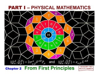
  • 1. BAAABAAA XQQPQQ βαβαµ µ βαβα εδσ == },{2},{ and&& From First Principles PART I – PHYSICAL MATHEMATICS January 2017 – R4.2 Maurice R. TREMBLAY BAAABAAA XQQPQQ βαβαµ µ βαβα εδσ == },{2},{ and&& Chapter 2
  • 2. Contents PART I – PHYSICAL MATHEMATICS Useful Mathematics and Infinite Series Determinants, Minors and Cofactors Scalars, Vectors, Rules and Products Direction Cosines and Unit Vectors Non-uniform Acceleration Kinematics of a Basketball Shot Newton’s Laws Moment of a Vector Gravitational Attraction Finite Rotations Trajectory of a Projectile with Air Resistance The Simple Pendulum The Linear Harmonic Oscillator The Damped Harmonic Oscillator General Path Rules Vector Calculus Fluid Mechanics Generalized Coordinates 2016 MRT The Line Integral Vector Theorems Calculus of Variations Gravitational Potential Kinematics of Particles Motion Under a Central Force Particle Dynamics and Orbits Space Vehicle Dynamics Complex Functions Derivative of a Complex Function Contour Integrals Cauchy’s Integral Formula Calculus of Residues Fourier Series and Fourier Transforms Transforms of Derivatives Matrix Operations Rotation Transformations Space Vehicle Motion Appendix 2
  • 3. Mass m is a property possessed by all material bodies. Classically, it is a property which describes the effort necessary in giving the body a change in motion. 2016 MRT Newton’s Laws aF m= Newton’s first law is a special case of the second law when F=0. It states that if no force acts on the particle, it will remain at rest or continue to move in a straight line with constant velocity. The equilibrium concept in statics is based on the first law, and the converse of the above statement requires that the resultant of all forces acting on a particle in equilibrium must be zero. The extension of Newton’s laws to a group of particles necessarily involves the action between particles. Actual bodies can be viewed as a group of particles, and to deduce the behavior of such bodies, he introduced Newton’s third law which states: For every action, there is an equal and opposite reaction. Thus if particle 1 exerts a force f12 on particle 2, particle 2 must exert a force f21 on particle 1, where f12 =−f21. 3 Its precise definition is embodied in Newton’s second law, which states that: For a given particle we can write F1/a1 =F2/a2 =F3/a3 =constant where F and a are in consistent set of units. The ratio F/a which is found to be constant for any given particle, is a property of the particle, which is designated as mass, labelled by m. We can therefore write Newton’s second law as: A particle acted upon by a force F will move with an acceleration a proportional to and in the direction of the force; the ratio F/a being constant for any particle.
  • 4. tav = 0 1 s 2 s 3 s 4 s 5 s 6 s 0 5 m/s 7.5 m/s 10 m/s 12.5 m/s Speed v(t): Time t: 2.5 F 2 2 1 tas= 0 5 m 11.25 m 20 m 31.25 m 45 m Distance s(t): 1.25 When a constant force F is applied to a mass m it will move with constant acceleration a. 0 2.5 m/s2 Acceleration a=|a|: 2 m/s2.5=a2.5 m/s22.5 m/s22.5 m/s22.5 fkBut if a friction force fk (=µN) is present (i.e., µ ≠ 0) it will oppose the acceleration. N =+mg Nµ µ 40≅ = gmfk 1 s 2 s 3 s 4 s 5 s … s Imagine that a mass m of 4 Kg (4⋅1000 g) is being pushed by a constant force F of 10 Newtons [N]. a) Calculate the uniform acceleration a of the mass m over a distance of 45 meters [m]. b) Represent the motion using a strobe graph in 1-second [s] time intervals and show the various distances s(t) and velocities v(t) corresponding to these time t intervals. Assume that there is no friction between the block and the surface (µ=0): Imagine a 4 Kg block of ice sliding on ice! 2 2 m/s Kg m/sKg Kg Newtons 5.2 4 10 4 10 = ⋅ ==⇒== a m a F a In this case, Newton’s 2nd law is simply F=ma. Dividing this equation by m on both side of the equality sign, we get: Every1s, astrobe ‘ ’ captures the motion of a 4Kg mass under an applied 10N ‘constant’ force… 2016 MRT The acceleration increases by 2.5 m/s (constantly) every second – 2.5 m/s /s! The acceleration due to gravity g is 9.8 m/s /s! 4 TAPE
  • 5. M M m h d T Mg +a T +a (1) (2) As an application of an accelerated motion consider Atwood’s machine. It was an apparatus that allowed a direct measurement of Newton’s second law. It could also be used to measure the gravitational constant g (we’ll use m/s2). Two equal blocks of mass M hang on either side of a pulley (see Figure). A small square rider of mass m is placed on one block. When the block is released, it accelerates for a distance h until the rider is caught by a ring that allows the block to pass. From then on the system moves at a constant speed which is measured by timing the fall through a distance d. Show that: 2016 MRT Decomposing the vertical components of the net force: 2 2 2 2 1 2 2 2 )2( th d m mM thm dmM g ⋅⋅ + = + = maMamgMgTF MaMgTMaMgTF y y −−=−−+= +=⇒+=−+= ∑ ∑ (2) (1) and finally for h to d, d =vt which implies v= d/t so we get g ! From 0 to h, v2 =+2ah which implies that a=v2/2h and: g h v m mM =      + 2 2 2 maMamgMgMaMg −−+=+ With T from Eq. (1) we put it into Eq. (2) to obtain: An Atwood machine. where t is the time moved at constant speed. In the lab, one only has to find this time t! (1) (2) 5 ga m mM gmamaM =      + ⇒=+ 2 2 so that:
  • 6. mg y Ncosθ N θ θ Nsinθ x fs As an application of a friction force let us consider the scenario depicted in the Figure. A car travels in a horizontal circle around a curve of radius R banked at an angle θ to the horizontal. If µs is the coefficient ofstatic friction, but assuming that µs tanθ <1 and that aR = (v2/R)êR, show that the maximum speed possible without sliding sideways is: 2016 MRT A car is traveling on a banked road at a constant speed v. We start by decomposing the components of the net force: 0sincos 0cossin =−−+= =−−−= ∑ ∑ θθ θθ cy csx FgmNF FgmfF From Eq. (1) above, we get since fs =µs N :     → → =⇔        − + = 0 0tan tan1 tan θµ µθ θµ θµ if if maxmax gR gR vgRv s s s s aR θ θµ θ θ cos sin cos sin gmNgmf F ss c + = + = whereas from Eq. (2) above, we obtain: θθ sincos cFgmN += Thus: θθµµ θ θµθµ tantan cos sincos gmFgm Fgm F css css c ++= + = and finally with Fc =maR =mvmax 2/R and we get vmax above.         − + =⇒+=− θµ θµ θµθµ tan1 tan )tan()tan1( s s cssc gmFgmF and then: (1) (2) 6
  • 7. Newton’s laws of motion were formulated for a single particle. If the mass m of a particle is multiplied by its velocity v, the resulting product is called the linear momentum: 2016 MRT vp m= The velocity v here is measured with respect to an inertial frame of reference so that, if the position of the particle is defined by its displacement vector r, the velocity is v=dr/dt. Newton’s second law states that: The time rate of change of momentum is equal to the force producing it, and this change takes place in the direction in which the force acts: p p F &== td d where the dot ‘⋅⋅⋅⋅’ is shorthand for d/dt. With m constant, this equation can also be written: rvF rrvv F &&& mm td d m td d td d m td d m td md ===      === or2 2 )( Newton’s first law, which forms the basis for statics, is a special case of the second law when the force F is zero. It states that: If the forces acting on a particle balance to give a resultant force of zero (i.e., F=p=0), the particle remains at rest (i.e., p=0), or continues to move in a straight line with constant velocity or momentum (i.e., p=constant). ⋅⋅⋅⋅ 7
  • 8. mm mm Impact (e=1) V1 V2> v1 v2< If the force F is multiplied by an infinitesimal amount of time dt and integrated, we get: 1212 )(2 1 2 1 2 1 2 1 2 1 vvvvvv vp F mmmmdmtd td d mtd td d td t t t t t t t t t t −=−===== ∫∫∫∫ The time integral on the left side of the equation is called the impulse of the force, so that the above equation states that: The change in momentum of a particle is equal to the impulse of the force acting on the particle. 2016 MRT Momentum before impact is equal to momentum after impact. When no energy is dissipated, the impact is elastic and e= 1 (∆V = ∆v), whereas for the completely plastic impact the relaxation impulse is zero and e =0. In general e depends on the material, shape and the velocities of the two bodies. When two bodies collide, a large force F(t) acts for a short time, and the impulse ∫Fdt exerted on the two bodies must equal and opposite according to Newton’s third law. Since impulse is equal to the change in momentum, for the two bodies considered together as a system, the impulses of collision cancel each other. Thus the change in momentum of the system is zero, and the momentum before impact must equal the momentum after impact. Energy however, is generally dissipated during impact, in which case the impulse during relaxation is less than the impulse during compression. ( ) ( ) approachofVelocity separationofVelocity ncompressio relaxation = ∆ ∆ = − − == ∫ ∫ V v VV vv F F 12 12 td td e The sequence of events is illustrated for e=1 in the Figure. 8 For central impact we let this ratio be e, the coefficient of restitution, and it can be shown that e is also expressible in terms of the velocities as:
  • 9. The moment about an arbitrary point O of the momentum p=mv=mR of a particle is: RrprL &m×××××××× ==o where R is the absolute velocity of m and r is drawn from O to P as shown in the Figure (a moment ∆t later, the particle is at P′). Differentiating the equation above, we obtain: Substituting R=Ro ++++r and noting that r××××r=0, this equation becomes: ⋅⋅⋅⋅ ⋅⋅⋅⋅ 2016 MRT Moment about O of momentum mR is r××××mR. ⋅⋅⋅⋅⋅⋅⋅⋅ Moment of a Vector RrRr pr L &&&&& mm td d ××××++++×××× ×××× == )( o ⋅⋅⋅⋅ ⋅⋅⋅⋅ ⋅⋅⋅⋅ ⋅⋅⋅⋅ ⋅⋅⋅⋅ rRRrL &&&&& mm ××××−−−−×××× oo = To establish the relationship between Lo and the moment Mo of the force F=mR (or sum ΣiFi) acting on m, we have: ⋅⋅⋅⋅ ⋅⋅⋅⋅⋅⋅⋅⋅ rRrrrRrRrM mm td d mm ××××−−−−××××++++×××××××× ooo )()( &&&&&&&&& === Substituting Mo =r××××mR into Lo = r ×××× mR– Ro ××××mr above, we can also write: ⋅⋅⋅⋅⋅⋅⋅⋅ ⋅⋅⋅⋅ ⋅⋅⋅⋅ ⋅⋅⋅⋅⋅⋅⋅⋅⋅⋅⋅⋅ rRLM &&& m××××++++ ooo = Generating the moment vector Mo on a diagram is hard to visualize in terms of this sum of the time rate of change of Lo, Lo, and the cross product of the time rate of change of both Roand mr, Ro ××××mr, at the same time. In the Space Vehicle Motion chapter, a physical description using angular rotations and moments of inertia will help us to better visualize the moment Mo in the case of the thrust misalignment of a rocket! ⋅⋅⋅⋅ ⋅⋅⋅⋅ ⋅⋅⋅⋅ 9 y x z R m Ro r O R ⋅ y x z R m Ro r Lo Lo R ⋅ t t + ∆t s s P P′ O′ Lo ⋅⋅⋅⋅ r⋅⋅⋅⋅ Ro ⋅⋅⋅⋅ r⋅⋅⋅⋅ Ro ⋅⋅⋅⋅ m m Mo Lo ⋅⋅⋅⋅ ⋅⋅⋅⋅ Ro ××××mr⋅⋅⋅⋅ Ro ××××r
  • 10. Several conclusions can be drawn now: oo LM &= 2. If point O is moving with constant velocity, Ro =0, and: 1. If point O is fixed in space, then Ro =Ro =0 and r=R, which results in the simplified equation: 3. If either Ro or r or Ro and r are parallel, again the simplified equations are valid; 4. If the system consists of more than one mass, labelled by i=1,2,… ,n, the second term of the equation Mo =d(r××××mr)/dt–Ro ××××mr obtained earlier becomes −Ro ××××Σimiri which is zero (Σimiri=0) when the point O coincides with the center of mass. The moment equation is then the same as in Case 2). ⋅⋅⋅⋅ ⋅⋅⋅⋅⋅⋅⋅⋅ ⋅⋅⋅⋅ ⋅⋅⋅⋅ ⋅⋅⋅⋅⋅⋅⋅⋅ which states that the moment is equal to the rate of change of the apparent moment of momentum (or angular momentum) expressed in terms of the relative velocity r; Fr rr r rrrM ×××× ×××××××××××× = === && & & m td d mm td d )(o ⋅⋅⋅⋅ ⋅⋅⋅⋅⋅⋅⋅⋅ ⋅⋅⋅⋅ ⋅⋅⋅⋅ ⋅⋅⋅⋅ ⋅⋅⋅⋅⋅⋅⋅⋅ ⋅⋅⋅⋅⋅⋅⋅⋅ 2016 MRT 10
  • 11. [9,6,−2] A(1,−3,2) P(4,−1,7) x y z r F Mo Let’s get right into the physics of the cross product: the Moment of a Vector! This time we will use the concept of the force vector to visualize the moment of a vector... The moment Mo will be independent of where r terminates on F or on its line of action. nFrM ˆ)sin(o ϕrF== ×××× 2016 MRT The moment of force vector Mo normal to plane of position vector r and force vector F is r××××F. ˆ Exercise: A force of 5 lb which acts through the point P(4,−1,7) in the direction of the vector [9,6,−2]. Find the moment of this force about the point A(1,−3,2). We consider a vector F and any point O in 3D space. If we draw a vector r from O to any point on F or on the line of action of F (see Figure) and form the cross product with r as the first vector, then the result will be a moment of force Mo about the axis through O in a direction perpendicular to the plane containing r and F, the direction of which is indicated by the unit vector n: 11 Mo nˆ r ϕ In a plane (e.g., 8½×11 paper) The vector Mo comes out of front of page. F O Solution: The position vector is r =(4 −1)i ++++(−1 +3)j ++++ (7−2)k = 3i ++++2j ++++ 5k and |r|=√(32 +22+52)= √(38)≈6 [ft] while the force vector is F=(9− 4)i ++++(6 −1)j ++++ (−2 −7)k =5i +5j−−−− 9k and |F|=5 [lb]. The formula for the moment is Mo = (|r||F|sinϕ )n but ϕ is unknown so we will have to compute Mo =r ×××× F= =(−18− 25)i −−−− (−27 −25)j ++++ (15 −10)k =−43i −−−−52j ++++ 5k and |Mo |=√(422 + 522+52)= √(4578)≈68 [lb⋅ft]. Since r •F=3⋅5 +2⋅5 +5⋅−9 =−20 = |r||F|cosϕ =6⋅5 cosϕ gives cosϕ =−20/30 so we get ϕ =132°. 955 523 ˆˆˆ − kji ˆ ˆ ˆ ˆ ˆ ˆ ˆ ˆ ˆ ˆ ˆ ˆ ˆ ˆ ˆ ˆ ˆ ˆ ˆ
  • 12. l=30 cm Biceps (Tension T) 4 cm θ = 10° d +ττττ wArm wBall FH FV T +g Humerus Radius Ulnaττττ d l As an application of a moment of force (here torque ττττ is used in a context of an applied weight w=−mg)letus considerthe scenario depicted in the Figure which shows a diagram of an arm and the biceps muscle. The muscle is attached at a point about 4 cm from the socket which acts as a pivot point. If a weight of 50 N is held in the hand, what is the ten- sion in the muscle? (Assume that the forearm is a horizontal uniform rod of weight 15 N and lengthl=30cm andthattheforce exertedby the muscle acts at10° to the vertical.) The Figure (ττττ out of page) shows the forces acting on the forearm, where FH and FV are the horizontal and vertical components of the force exerted by the pivot of the forearm. 2016 MRT Since the muscle is close to the pivot point, it must exert a force much larger than the weight of the ball (i.e., using wBall =mg: 50 N =m⋅ 9.8m/s2 ⇒ m ≅ 5 kg). By taking torques about the pivot we avoid the force exer- ted by the pivot. Thus, using the components of the torque ττττ =r ××××F (i.e., with its magnitude being |ττττ|=|F||r|sinθ for d, l and T instead) explicitly under static equilibrium conditions: 0)1()3.0()50()1( 2 3.0 )15()1()04.0()10cos( 090sin90sin 2 90sincos =⋅⋅−⋅      ⋅−⋅⋅= =⋅⋅−⋅⋅−⋅⋅+=∑ mN m Nm BallArm o ooo T lw l wdT θτ Thus, T = |T|=438 N, which is considerably greater than the weight wBall (i.e., 50 N or ∼10×). As for the forces FH and FV : V y H x wwTF TF F F ==−−= −−= === = ∑ ∑ NNNN NN BallArm 3665015)10)(cos438( cos 76)10)(sin438( sin o o θ θ 0wlw l Tdτ ==∑ BallArm ××××−−−−××××−−−−××××++++ 2 12 Humerus
  • 13. m m ev N θ ⋅⋅⋅⋅ l CM Problem: A dumbbell idealized by two masses on a stiff, weightless rod of length l is dropped without rotation, and the left mass strikes a ledge with velocity v. Assume a coefficient of restitution to be e (e.g., e=1 collide elastically, e<1 collide inelastically and for e=0, objects effectively stop at the collision, not bouncing at all). Determine the angular rotation of the dumbbell immediately after the impact. Solution: The dumbbell immediately after impact is as shown. ⋅⋅⋅⋅ )2( 2 2 mv l vemtdN −−      −=∫ θ& where N is the normal force and the change about the angular momentum about the center of mass is equal to the moment about the center of mass of the impulse ∫Ndt and is: θ& 2 2 2 2       =∫ l mtdN l Eliminating the impulse integral, the angular velocity immediately after the impact is: )1( e l v +=θ& 2016 MRT The velocity vCM of the center of mass immediately after the impact is ev−(l/2)θ, and the change in the linear momentum mv is: 13
  • 14. The basic concepts of mechanics are space, time, and mass(or force),which are more or less understood intuitively by most beginning students. To be useful for quantitative analysis, however, these notions must be viewed as mathematical concepts related to each other by fundamental laws. Such a formulation was introduced by Newton in his three laws of motion which have become the foundation for the classical mechanics or Newtonian mechanics. Although the likes of Le Verrier or Herschel would be jealous! Newton’s laws were formulated for a single particle and our notion of a particle is that of a material body of infinitely small dimensions. In mechanics we can expand this notion to include any material body whose dimensions are small in comparison with distances or lengths involved in defining its position or motion. Thus planets can be considered to be particles when their position in the solar system is taken under consideration. Gravitational Attraction In defining the position of a particle in space, a frame of reference is necessary. For this purpose, three perpendicular lines intersecting at a common point called the origin are adequate. The position of the particle can then be defined in terms of distances along these lines. Each component is squared then summed and the result square- rooted to give a position vector. To describe the motion of a particle, the concept of time is required. By noting the position of the particle as a function of time, its motion (e.g., described by its displacement, velocity, and acceleration) is completely defined. Force is known to us intuitively as a push or a pull which is represented by the action of one body on another, exerted by contact or through a distance as in the case of the gravitational (or electromagnetic) force. To describe a force, it is necessary to know its magnitude, its direction, and its point of application. 2016 MRT 14
  • 15. PT′ r R Q T t m Q′ 1444442444443 D R′ The most interesting case of gravitation attraction is, of course, the attraction exerted by the Earth. We shall take the Earth to be a solid sphere of mass M⊕ per unit volume (and surface radius Rs) and calculate the force that the sphere exerts on a mass m. The calculation of the gravitational attraction that a thin spherical shell exerts poses a problem in itself. Suppose that an object of mass m is located at point P (see Figure) which is D units from the center O of the shell. The shell has a thickness that we shall denote by t. The parts of the shell are all at different distances from P, and so we cannot apply the law of gravitation (i.e., F=GmM⊕/r2 below) at once to the shell and the mass m. The force which the Earth exerts on any object at any distance from the Earth’s center is given by the famous axiom of physics known as Newton’s law of gravitation. This law states that any two objects in the universe attract each other, and the force with which each attracts the other is given quantitatively by the formula: In this formula G =6.674×10⁻¹¹ N⋅(m/kg)2 is the gravitational constant; it is the same number no matter what the masses involved and no matter what the distance r between them. The quantities m and M are the masses of the two objects.         === ⊕ 2 s ss2 R MG ggm r Mm GF if An object of mass m is located at point P. 2016 MRT 15 We can regard the shell as composed of small zones. Thus the circles QR and Q′R′ bound a zone on the outer sphere of the shell, and if we take this zone to have the thick- ness t of the shell, we may regard the shell as composed of a number of such zones. O
  • 16. O P r R′ R Q′ Q T m t f T′ U A U′ θ dθ ∠OPQ a dV D r aD PQ OA PQ AP OPQ θcos )cos( − = − = =∠ Let us consider, then, the attraction exerted by any one zone on the mass m. We think of the zone (see Figure) as made up of equal little pieces such as U′U TT′, each of which pulls the mass m. What we should seek is the component PO that each piece of the zone exerts. These components can all be added to obtain the attraction caused by the zone because they are in the same direction. The little pieces of any one zone all make about the same angle with PO, namely the angle∠OPQ, and each piece is the same distance r from the mass m. Hence the compo- nent of the force f along PO that each piece of the zone exerts is the same. If we let ∆V be the volume of each piece of the zone, then M∆V is the mass of the piece (we will also keep M as unspecified from now on). The force exerted by this piece along PO is: The sum of all these components is: where θ is the angle shown in the Figure. )cos(2 OPQ r mMG dV ∠⋅ An object of mass m is located at point P. 2016 MRT )cos( )( 2 OPQ r mMVG ∠ ∆ where V is the volume of the zone. This volume is approximately t times the area of the zone (i.e., dV=t⋅dA). The area is approximately the circumference of the circle QR multiplied by the arc length QQ1. This area is: θθθ daadaQAAd sinπ2π2 =⋅⋅= 16 OP
  • 17. Then the component along PO of the force f exerted by the entire zone is: since dV=t⋅dA and dA=2πasinθadθ. If we denote this component of f by f , we get: r aD PQ OAOP PQ AP OPQ θcos )cos( − = − ==∠ 2016 MRT )cos(sinπ2)cos()cos( 222 OPQ r mGM daatOPQ r mGM AdtOPQ r mGM Vd ∠⋅⋅=∠⋅⋅=∠⋅ θθ Let us now find an expression for ∠OPQ in this last equation. We have from the previous Figure that: )cos( sinπ2 2 2 OPQ r datmGM f ∠ ⋅ = θθ where D is the distance from the center of the sphere, O, to the mass m at P. Then: r aD r datmGM f θθθ cossinπ2 2 2 − ⋅ ⋅ = This last equation contains two variables (i.e., θ and r) and we must eliminate one of these to obtain the integrand of our ultimate definite integral. Fortunately, the law of cosines, c2 =a2 +b2 −2abcosC, applied to triangle OPQ furnishes us with the relation: θcos2222 aDDar −+= This equation defines r as a function of θ. 17 ab c A B C ra D θ≡ →
  • 18. By differentiating r2 =a2 +D2 +2aDcosθ with respect to θ, we obtain: To eliminate the remaining term in θ, we again use r2 =a2 +D2 +2aDcosθ. From it we have that: 2016 MRT θθ dDardr sin= The use of this relation to replace asinθ in our last equation for f yields: r aD rD rdratMmG f θcosπ2 2 − ⋅ ⋅ = θθ cos 2 cos22 222 2222 aD D aDr DaDaDr −= −+ ⇒−=−+ If we use this result in our result for f above, we have: rd r aDr D atGmM rf 2 222 2 π )( −+ ⋅ ⋅ = The quantity f(r) is the attractive force along PO which is due to the single zone formed by QRR′Q′. To obtain the attractive force due to the entire shell, we must first sum all elements of the form f(r) above one for each zone, and then let the number of zones become infinite while the width dr (or ∆r) of each zone approaches 0. If we visualize the various zones that fill out the spherical shell in the first Figure, we see that r will range from the value PT for the nearest zone to P to PT′ for the farthest zone from P. Then r ranges (i.e., the bounds of integration) from D−a to D+a. 18
  • 19. Then our definite integral for the attractive force of the entire shell is: This integral is readily evaluated. It is, first of all, the sum: 2016 MRT ∫∫ + − + −         − + ⋅ == aD aD aD aD rd r aD D atGmM rdrfF 2 22 2 1 π )( The results of the integration are: ∫∫ + − + − ⋅− ⋅ +⋅ ⋅ aD aD aD aD rd r aD D atGmM rd D atGmM 2 22 22 1 )( π 1 π By factoring D2 −a2 and by other simple algebraic steps (Exercise), we obtain:       − + + − − ⋅ +−−+ ⋅ aDaD aD D atGmM aDaD D atGmM 11 )( π )]()[( π 22 22 Then: )]()()()[( π 2 aDaDaDaD D atGmM ++−−−−+ ⋅ 2 2 π4 D atMGm F ⋅ = Because the surface area of a sphere of radius a is 4πa2 and because the mass per unit volume of the sphere is M, the quantity Mt ⋅4πa2 is the mass of the shell. The quantity m is the mass at P, and D is the distance from the center of the shell to P. 19
  • 20. O P mx D dx R The force F is exactly what one would obtain by regarding the mass of the shell as concentrated at the center of the shell and by applying the law of gravitation to the two masses m and Mt⋅πa2 separated by the distance D. In other words, a spherical shell acts, insofar as its gravitational attraction on an external mass is concerned, as though the mass of the shell were concentrated at the center (e.g., you can call that Gauss’ theorem for gravity – technically expressed as ∫∫S g•dS=−4πGM with g=−∇∇∇∇φ). We are now able to consider the gravitational force that a solid sphere of radius R exerts on an external particle (point mass) of mass m. We shall regard the sphere as a sum of n spherical shells (see Figure). However, in place of the notation t for the thickness of each shell we shall use the quantity ∆D or dx. An object of mass m is located at point P. 2016 MRT We did already show that the gravitational attraction of a thin shell may be computed by regarding the mass of the shell as concentrated at its center. Hence, with F= GmMt⋅4πa2/D2, the force that the typical shell exerts on the particle of mass m is: xd D xGmM xdxF ⋅ ⋅ =⋅ 2 2 π4 )( where D is the distance OP, that is, the distance from the center of the location of the particle. The calculations of the gravitational force exerted by the Earth is not really disposed of by all the previous or following text, for the Earth is not a sphere but an oblate spheroid, that is, one type of ellipsoid and to, say, calculate the moon’s motion the elliptical shape must also be taken into account! 20
  • 21. To obtain the gravitational force exerted by the solid sphere, we sum the forces exerted by the n concentric shells while the width of each shell approaches 0. Such a limit of a sequence of sums is a definite integral. To write down the definite integral, we need only the additional knowledge that x varies from O (i.e., 0) to R. If we let F be the force exerted by the solid sphere, then: or: 2016 MRT ∫ ⋅ = R xd D xGmM F 0 2 2 π4         =        ⋅ = ⋅ = ∫ 3 π4 3 π4π4 )( 3 2 3 20 2 2 MR D GmR D GmM xdx D GmM RF R This result has a very simple physical interpretation.The quantity 4πR3M/3 is the mass of the entire sphere. Because D is the distance from the center of the sphere to the particle at P, we see that the whole sphere acts on the external particle as though the sphere’s mass were concentrated at the center. The usual law of gravitation applies to the two masses with the distance between them the distance from the center of the sphere to P. The question also arises as to how does the Earth act on a particle inside (e.g., ass- ume that a tunnel is dug through the Earth to reach Australia)? If we were to make the calculation we would find that a thin spherical shell exerts no attractive force on any point mass or particle inside the shell. This also applies to shells of any thickness, i.e., even a shell of finite thickness exerts no force on a particle interior to it! 21
  • 22. From his interest in astronomy, and from the calculation outlined above to show that all the mass is as if it were concentrated at the center, Newton formulated the law of gravitation between two particles. The law states that any two particles attract one another with a force of magnitude: 2016 MRT 2 21 r mm GF = where m1 and m2 are the masses of the particles 1 and 2, r is the distance between them, and G is the universal constant of gravitation. gmw = and by comparison with the previous equation, we arrive at the result g=GM⊕/R⊕ 2. We find then that the acceleration of gravity g will vary inversely with R⊕ 2. Since m is a pro- perty of the body which is fixed, its weight will then vary with g and R⊕, and so we find a given body weighing somewhat different amount at different places on the Earth’s surface. At the Earth’s surface g=gs is nearly 32 ft/sec2 [CGS] or 10 m/s2 [MKS]. 22 Application of this law to a particle on the Earth’s surface gives us an understanding of the relationship existing between mass and weight. Letting m1 = M⊕ and m2 =m be the mass of the Earth and that of another body as the Earth’s surface, a distance equal to the radium r=R⊕ from the center, the attraction of the Earth on the body, which is called the weight, w, is given by interpreting the above equation as w=m(GM⊕/R⊕ 2)! If this force is not opposed to a support of some kind, the body will fall toward the center of the Earth with an acceleration g. Thus from Newton’s second law, we can write:
  • 23. We know that the force of gravity varies from place to place on the surface of Earth. There are two reasons behind this variation: the shape of Earth and the rotation of Earth. The Earth is not a perfect sphere, but bulges at the equator. Therefore if a body is taken from pole to equator its distance from the centre of the Earth will change. Consequently, the gravitational force also varies, although totally imperceptible to us on any given day! 2016 MRT 2s ⊕ ⊕ = R M Gg Consider the variation of gs when a body moves distance upward or downward from the surface of Earth. Let gs be the value of acceleration due to gravity at the surface of Earth and gh at a height h above the surface of Earth. If the Earth is considered as a sphere of homogeneous composition, then gs at any point on the surface of the Earth is: 23 Now we will determine the value of gs at a distance R⊕ +h from the center of the Earth. The acceleration due to gravity is: 2 )( hR M Ggh + = ⊕ ⊕ Then: 2 2 22 2 2 2 s )()( )(         + = + =⋅ + = + = ⊕ ⊕ ⊕ ⊕ ⊕ ⊕ ⊕ ⊕ ⊕ ⊕ ⊕ ⊕ hR R hR R M R hR M R M G hR M G g gh
  • 24. Pushing now to simplify things we get by dividing numerator and denominator by R⊕: 2016 MRT Using the binomial theorem: 24 and considering the replacement of x and n by h/R⊕ and −2, respectively, to obtain: which means that the value of g at a height h above the surface of Earth, gh, is 1−2h/R⊕ times that of gs, the acceleration due to gravity at the surface of Earth (i.e, R⊕): 222 s 1 1 1 − ⊕⊕⊕ ⊕         +=        + =        + = R h RhhR R g gh xnx n +≅+ 1)1( ⊕ −≅ R h g gh 2 1 s s 2 1)( g R h hggh         −≅= ⊕ If the height h above the surface of Earth is about half the Earth’s radius, ½R⊕, away then the value of Earth’s gravity at that height is g½R⊕ =(1−1)gs=0 (i.e., total weightlessness). At half that distance, ¼R⊕, you would only feel half your weight since g¼R⊕ =(1−½)gs=½gs.
  • 25. gh R⊕ gs h • h R(φ) Space Shuttle Orbit ti tf = ti + T • • •O gs is the value of g at Earth’s surface (9.807 m/s/s or m/s2), R⊕ is the radius of the Earth (6.38×10⁶ m), h is the altitude above Earth [m], gh is the value of g at altitude h [m/s/s]. The percentage difference in radii is 1.0025%! These different values for the Earth’s radius is a characteristic of the Earth’s oblateness (i.e., the Earth is an oblate spheroid!) The Earth’s equatorial radius of curvature in the ‘meridian’ is b2/a or 6335.437 km. The Earth’s ‘polar’ radius of curvature is a2/b or 6399.592 km. Difference is ∆ ≅ 1%! The Earth’s radius at a geodetic latitude,φ, is given by the radius of the Earth formula: = gsgh 22 2222 )sin()cos( )sin()cos( )( φφ φφ φ ba ba RR + + ==⊕ 2016 MRT 2         +⊕ ⊕ hR R 25 The plot of: in Excel shows that gh will decrease linearly with altitude (e.g., The space shuttle reaches an altitude of 300 km). C e l l gh =gs*(R/(R+h))^2
  • 26. So far we have avoided one very important question regarding the frame of reference used in the measurement of the motion. 2016 MRT 26 Newton assumed that there was a frame of reference whose absolute motion was zero. He considered such an inertial frame fixed relative to the stars to be one of absolute zero motion, and his laws of motion to be valid when referred to such a reference. Controversies regarding the existence of such reference frames of absolute zero motion led to the formulation of the theories of relativity for which Newtonian mechanics is a special – or ‘limited’ or even better coined as the ‘effective limit’ – case. In arriving at the concept of weight, it was necessary to measure gs relative to the surface of the Earth which is not at rest. Thus the acceleration of the Earth’s surface due to its rotation must be accounted for in a more exact analysis. For many problems this error is insignificant, in which case the Earth’s surface will be found to be an adequate reference. There are other problems, however, such as navigation for space flight, where the Earth’s surface cannot be considered stationary. In general, problems in space dynamics are involved with rotating and accelerating coordinates, and the subject of relative motion and transformation of coordinate play an important role.
  • 27. Finite angular rotations of a rigid body do not obey the law of composition (which states that the sum of two vectors is represented by the diagonal of a parallelogram formed by the two vectors as sides). It has magnitude equal to the angles of rotation, which can be directed along the axis of rotation. However, two such rotations along different axes are not commutative and will not add up to the diagonal of a parallelogram (e.g., Pick up an iPhone and lay it flat in your right hand so that your fingers can wrap around it. Rotate it 90° about the 1- and 3-axes with your left hand. You need to hold it up sideways! Then repeat the procedure in the reverse order. You will need to hold it up facing you! Thus finite angular rotations are shown to be non-commutative: 1⋅3≠3⋅1) Infinitesimal rotations however can be shown to be commutative (i.e., R⋅R−R⋅R=0 so here we have 1⋅3=3⋅1⇒1⋅3−3⋅1=0) and to possess all the properties of a vector. 2016 MRT The angular velocity represented by a vector. To show this, consider the displacement of a point P(r) due to two infinitesimal rotations ω1 dt and ω2 dt about any two axes, where ω1 and ω2 are their respective rotational speeds. Let the direction of each of the axes of rotation be indicated by unit vectors ê1 and ê2 as shown in the Figure, and we will perform the rotations in the order 1 and 2, then repeat in the reverse order to examine the final result. Because of the infinitesimal rotation (ω1 dt)ê1, the end of the displacement vector r defining the position P will be displaced to P′ by an amount (see Figure): re ××××11 ˆ)ω( td and the new position is defined by the vector (see Figure): rerr ××××++++ 111 ˆ)ω( td= Finite Rotations ê1 r ω1 r1 O ê2 ê3 ω2 ê1 r ê1×××× r P P (ω1 dt)ê1×××× r 27 P′
  • 28. r1 ω2 r2 P ê1 ê2 O ê3 ω1 r ê1 r Next allow the second infinitesimal rotation (ω2dt)ê2, starting from P′, in which case the final position is P(r2) and is defined by the vector r2: reererer rerererrerr ××××××××++++××××++++××××++++ ××××++++××××++++××××++++××××++++ 11222211 11221112212 ˆ)ω(ˆ)ω(ˆ)ω(ˆ)ω( ]ˆ)ω([ˆ)ω(]ˆ)ω([ˆ)ω( tdtdtdtd tdtdtdtd = == 2016 MRT Neglecting the second-order term (i.e., ω1ω2(ê2××××ê1××××r)dt2) above, we arrive at the result: tdtd rrreerr ××××ωωωω++++ωωωω++++××××++++++++ )()ˆωˆω( 2122112 == since ωωωωn=ωnên. If we repeat the operation in the reverse order, we will find the equation for r2 to be identical to the case above, indicating that infinitesimal rotations are commutative (at least to first-order since we neglected the second-order – or quadratic – term.) 28 P′
  • 29. ê2R(ϕ)ê2 R(ϕ)ê1 ê1 O ϕ ϕ You can skip this… Consider a system symmetric under a rotation in a plane, around a fixed point O. If we adopt a Cartesian coordinate frame on the plane with ê1 and ê2 as the other normal basis vectors (see Figure). Denoting the rotation through the angle ϕ by R(ϕ), we obtain by elementary geometry (see the Matrix Operations chapter): ϕϕϕϕϕϕ cosˆsinˆˆ)(sinˆcosˆˆ)( 212211 eeeeee ++++++++ −== RR and R(ϕ) has interesting properties such as two rotation operations can be applied in succession, resulting in an equivalent single rotation R(ϕ2)R(ϕ1)=R(ϕ2+ϕ1) (i.e., techni- cally here, R(ϕ1) goes first then R(ϕ2) next) but R(ϕ1)R(ϕ2)≡R(ϕ2)R(ϕ1) which equates to reversing the order of operation of the rotation with no change in the outcome! A rotation by and angle ϕ of two unit vectors ê1 and ê2 in a plane. J is the generator of rotation. The differentiability of R(ϕ ) in ϕ requires that R(dϕ) differs from R(0)= 1 (i.e., the identity – or ‘nothing happens’ or it ‘ends up the same’) by only a quantity of order dϕ which we define by (i2 =−1): JdidR ⋅−= ϕϕ 1)( 2016 MRT where the quantity J is independent of the rotation angle dϕ. Next, consider the rotation R(ϕ +dϕ), which can be evaluated in two ways: ϕ ϕ ϕϕϕϕ ϕϕϕϕϕϕϕϕϕ d Rd dRdR JRidRJdiRdRRdR )( )()( ])([)()1)(()()()( +=+ −+=⋅−==+ Comparing the two equations, we get the differential equation: 0)( )( )( )( =+⇒−= JRi d Rd JRi d Rd ϕ ϕ ϕ ϕ ϕ ϕ with solution R(ϕ )=exp(−i ϕ J) and boundary condition R(0)=1.       − =⇒    −= += ϕϕ ϕϕ ϕ ϕϕϕ ϕϕϕ cossin sincos )( cosˆsinˆˆ)( sinˆcosˆˆ)( 212 211 R R R eee eee ++++ ++++       − −− =             − ==− ϕϕ ϕϕ ϕ ϕ ϕ ϕ ϕ ϕ ϕ ϕ ϕ ϕ ϕ sincos )cos(sin cossin sincos )( )( d d d d d d d d d Rd JRi       − =      + −       − − ϕϕ ϕϕ ϕϕ ϕϕ sincos cossin 0 0 cossin sincos i i i       + − = 0 0 i i JJ istheif generator 29
  • 30. vx i vy j −kvy j −kvxi Gravity Velocity v Air Resistance −mg Fair=−kv Below is a free body diagram (not to scale) for a projectile that experiences air resistance and the effects of gravity (the dashed vectors are the x and y components of velocity and air resistance). Here we assume that the air resistance is in the direction opposite of the projectile’s (e.g., baseball) velocity. Trajectory of a Projectile with Air Resistance When the velocity of the projectile is 4 m/s, the air resistance is 7 N. When we double the velocity to 8 m/s, the air resistance doubles to 14 N accordingly. In this case, k=7/4= 1.75 N⋅s/m – i.e., 75% more resistance to travel than without air resistance! We can write that the air resistance is an inverse linear function in the velocityv with k as the drag coefficient (N.B., Atmospheric drag is highlighted below but not considering uncertainties in atmospheric fluctuations, Earth’s oblateness, &c. If we consider only the cross-sectional area A perpendicular to the direction of motion, the dimensionless drag coefficient CD associated with A, and other parameters such as the speed of the mass m relative to the atmosphere va and the atmospheric density ρ at the mass’ altitude): 2016 MRT tCoefficien Ballistic 1 2 1 =   −=−= mg ACD aD vACvkF ρAir ˆ ˆ ˆ ˆ 30
  • 31. Neglecting the Magnus effect (i.e., basketball rotation via (16/3)π2rbasketball ρ ωωωω××××v) the formula for calculating the drag force of an object moving through a fluid is thus: 2 2 1 aDD vACF ρ= where ρ is the density of the fluid and A is the area of the ball. If the fluid is air, then for air at sea level we have ρ=1.2 Kg/m3.The coefficient of drag for this shape is CD ~0.5 (i.e., for most spheres for most sports conditions.) For a basketball with v=20 m/s and area A=0.046 m2, we then have FD =½⋅1.2⋅400⋅0.5⋅0.046=5.5 N. The weight of the ball is w=mg=4.5⋅1.31=6 N so this is comparable to drag force. CD is not a fixed number but depends on Reynolds number and surface smoothness. This calculation of drag force is close enough. Given a range R of a ball launched at 45 degrees, from kinematics we have R=vo 2/g where vo is the launch velocity assuming the ball is launched from the height of the basket – i.e., a tall man with jump shot. For a 3 point shot, R=24 feet=7.3 m. Given g=10 m/s2, vo =√(Rg)=√(7.3⋅10)=8.5 m/s. For a 3 point shot, launch velocity in vacuum is 8.5 m/s so the drag force is FD =(8.5/45)2=0.036≥3.6% of its weight. Since the range varies as the square-root of the kinetic energy,√T, and that the drag force is proportional to the loss of total energy, the range is reduced by about 1.8% or 0.13 m (i.e., 13 cm). The basket has an allowance of 0.15/2 m so the loss of range doesn’t cause a clean miss! The players obviously practice shooting at the actual target hoop to get used to the way it looks and to get the feel for the launch velocity from experience. For shorter shots, the change in range is considerably smaller due to the launch velocities which are much smaller than that of the terminal velocity. 2016 MRT 31 2
  • 32. Now back to the resistance problem. Here we assume that the air resistance is in the direction opposite of the projectile’s velocity. We can write that the air resistance is an inverse linear function in the velocity v with k as the drag coefficient: because initial assumptions of proportionality implies that the air resistance and the velo- city differ only by a constant arbitrary factor, and that when v is increased by a factor of, say, p, the air resistance increases by a factor of p also. vF k−=Air To derive relationships to represent the motion of the particle, we first apply Newton’s Second Law (i.e., the sum total of all vector forces F=FWeight++++FAir equals the product of the scalar mass m by its vector acceleration a: ΣF=ma=m(axi++++ay j)=0) for both the x and y components: ˆˆ The weight mg term is positive because the value of g is already negative and subtracting it would result in a positive number. Note that acceleration is just the derivative (i.e., infinitesimal rate of change) of velocity with respect to time (i.e., a=dv/dt). 0=+=∑ x x x kv dt dv mF 2016 MRT 32 0=−+=∑ mgkv dt dv mF y y y and
  • 33. Solving the first of these equations, mdvx /dt=−kvx, is an elementary problem in solving differential equations that we will show next, starts by re-writing it in the standard form: and we get: where A is an arbitrary constant. The quantity exp[−∫p(x)dx] is referred to as the integrating factor. xdxp y yd yxp xd yd )(0)( −=⇒=+ ∫− =⇒−== ∫∫ xdxp Ayxdxpy y yd )( e)(ln nIntegratio tables We now multiply the original equation dy/dx+p(x) y=q(x) by the inverse of the integrating factor. On multiplying it by exp[+∫p(x)dx] we obtain: ∫∫ =      + xdxpxdxp xqyxp xd yd )()( e)(e)( 2016 MRT We now solve the corresponding homogeneous equation (i.e., with q(x)=0): 33 this differential equation in vx is of the general form dy/dx+p(x) y=q(x) and is called a first-order linear differential equation. Notice the similarity of dy/dx+p(x) y=q(x) with dvx /dt+(k/m)vx=0 by making the changes y →vx, x →t, p(x)→k/m and q(x)→0. 0=+ x x v m k xd vd
  • 34. Since: our last equation (i.e., [dy/dx+p(x) y]exp[∫p(x)dx] =q(x)exp[∫p(x)dx]), may be written as: Integrating this equation, we get: or: This is the general solution of the differential equation dy/dx+p(x) y=q(x). where C is an arbitrary constant of integration. Finally, when p(x) is independent of x it is a constant, say po, and the differential equation is dy/dx+po y=0 and its solution becomes y=Cexp(−po ∫dx)=Cexp(−po x). Note this since we will be using it again soon. 2016 MRT ∫∫ = xdxpxdxp xqy xd d )()( e)(]e[ ∫∫∫∫       +=+=⋅ xdxpxdxpxdxpxdxp yxp xd yd xpy xd yd y xd d )()()()( e)(]e)([e]e[ Cxdxqyyd xdxpxdxpxdxp +== ∫∫ ∫∫∫ )()()( e)(e]e[ ∫−∫∫− += ∫ xdxpxdxpxdxp Cxdy )()()( eee )(xq ∫− = xdxp Cy )( e When q(x)=0, the differential equation reduces to dy/dx+p(x) y=0 and it has the solution: 34
  • 35. As a simple application let us consider (Jacob) Bernoulli’s (1654-1705) equation: This differential equation is non-linear since it contains a non-linear term in the dependent variable, yn, but it can be reduced to the linear form. To reduce dy/dx+p(x) y= q(x)yn to the linear form, we first make a change of variable. Let: so that: On multiplying dy/dx+p(x) y=q(x)yn by (1−n)y−n, we obtain: which is the linear form that was sought. This differential equation is the required linear form. It can be solved by use of the method just outlined and its solution is (N.B., n>1): 2016 MRT ( )1)()( ≠=+ nyxqyxp xd yd n n yz − = 1 xd yd yn xd zd n− −= )1( )()1()()1( xqnzxpn xd zd −=−+ In terms of the variable z, we write: )()1()()1()1( 1 xqynxpyn xd yd yn nn −=−+− −− ∫−−∫−∫−− +−= ∫ xdxpnxdxpnxdxpn Cxdxqnz )()1()()1()()1( ee)()1(e 35
  • 36. Now, I could not pass the chance of discussing a simple application of the first-order linear differential equation – that of radioactive decay. Radioactivity was discovered in 1896 by Becquerel (1852-1908) while working on phosphorescent materials. In the ra- dioactive decay of unstable nuclei, we find that the process is governed by the following differential equation. The time rate of change of N(t) is proportional to decreasing N(t): where N(t) represents the number of parent atoms present at time t, λ is the decay (or disintegration) constant which is characteristic of the particular element involved, and the negative sign is used to indicate that the number of parent atoms decrease with time. where the minus sign indicates that dN is always negative or decreasing. The probability of disintegration per unit time (i.e., seconds [s]) λ is: 2016 MRT ( )o)0()( )( NtNtN td tNd ==−= λ N Nd −=tiondisintegraofyProbabilit If N represents the number of atoms present at a given time t and dN represents the number of disintegrations during an infinitesimal time interval dt, then: constant=−= − = td Nd Ntd NNd 1)( λ where λ is identified as the disintegration constant. The activity of a sample is defined by A=|dN/dt|=λN disintegrations/s and represents the rate at which disintegrations of nuclei occur – units being the Curie [Ci] which represents 3.70×10¹⁰ disintegrations/s. 36
  • 37. The λ=−(1/N)dN/dt equation can be rewritten in a slightly different form, and if there are No initial atoms at t=0, then: where ln is the natural logarithm (N.B., ln(ξ1)±ln(ξ2)=ln(ξ1ξ2 ±1)) whereas in exponential form it becomes: or, in logarithmic form: 2016 MRT tttNtN NtN N tN λλλ −−− =⇒== e)(e )( ee o o ])([ln o or where exp(lnξ )=ξ. When the above equation (i.e., N=Noexp(−λt)) is multiplied through by λ, it becomes λN=λNoexp(−λt) where λNo =Ao is the initial activity and λN=A is the activity at some time t. This gives for the activity: t AtA λ− = e)( o t N tN NtNNtd N Nd N N t t N N λλ −=      ≡−=−= ∫∫ = o o 0 )( ln]ln[)](ln[ln o o or tAA λ−= olnln The half-life T½ of a radioisotope is defined as the elapsed time in which the number of atoms decays to one-half the initial number, or the time in which the activity drops to one-half the initial activity. When t=T½, then, the number of atoms of a given kind present is N=½No and, from N=Noexp(−λt), we get ½No =Noexp(−λT½) or ½=exp(−λT½). By taking the logarithm of both sides gives −ln2=−λT½ or the half-life is T½=ln2/λ = 0.693/λ. 37
  • 38. 20 40 60 80 Naturallogarithmofactivity 12.0 11.0 10.0 9.0 8.0 7.0 T½ lnA = lnAo − λt Time, t [days] lnAo ln½Ao (0,10.8) (78,0) 20 40 60 Ao Activity,A[(counts/min)×10−3] 50 40 30 20 10 0 ½Ao T½ 14.3 A =Ao e−λt Time, t [days] Here is a typical example that is meant to portray in graphic form an exponential function and a linear slope as well as a practical way to figure out an isotope’s T½. Then we can use T½=0.693/λ to calculate the half-life of 32P as being T½ 32P =14.3days! 1 days− == − − = 0.049 78 8.3 078 0.78.10 λ 2016 MRT The curve shows the exponential decay of the Phosphorus-32 isotope, which has a half-life of 14.3 days. The sample originally had an activity of 50,000 disintegrations/min. When the natural logarithm of A=Aoexp(−λt) is taken, it gives lnA=lnAo −λt. When lnA is plotted against t, it gives a straight line with a slope equal to −λ. The exponentialdecay() ofactivityof thePhosphorus-32 isotope(32P with 15 protons and 17 neutrons) is shown in the Figure - Left. If the natural logarithm of the activity is plotted against time as in the Figure - Right, according to lnA=lnAo −λt it will produce a straight line () that has a slope equal to −λ. The disintegration constant λ for 32P from the slope of the line in the Figure - Right is: 38
  • 39. Inductor Inductance: L Units: Henry [H] Voltage drop: td Id L L I → C Resistor Resistance: R Units: Ohm [Ω] Voltage drop: IR R Capacitor Capacitance: C Units:Farad [F] Voltage drop: q C 1 I → I → L C RE I → q E(t) ∼∼∼∼ or q Problem: Derive the expression for the current in the circuit in the Figure if it is compri- zed of a single loop series containing only an inductor and a resistor (i.e., no capacitor). Solution: In reviewing the circuit, we see that the current (e.g., after a switch is closed) is denoted I(t) and the charge on a capacitor at time t is denoted q(t). The letters L, C, and R are known as the inductance, capacitance, and resistance, respectively, and are gene- rally constants. Now according to Kirchhoff’s second law, the voltage E (constant) on a closed loop must equal the sum of the voltage drops in the loop. Since the current I(t) is related to the charge q on the capacitor by I=dq/dt, we can add the three voltage drops: 2016 MRT An LRC-series circuit: a resistor, inductor and capacitor. The current I(t) and charge q(t) are measured in amperes [A] and coulombs [C], respectively. Setting the sum of these drops to the impressed voltage E, we obtain a second-order differential equation in the charge q(t): )( 1)( )( )()( 2 2 tq Ctd tqd RtIR td tqd L td tId L and, == Etq Ctd tqd R td tqd L =++ )( 1)()( 2 2 This equation is quite complicated and truthfully, it does not provide an answer to our question since current is not explicit! ( )capacitornoEtIR td tId L =+ )( )( To answer the question, we must find a differential equation in the current I(t) . Furthermore, when we remove the capaci- tor, the differential equation reduces to a first-order linear diffe- rential equation leads us to this differential (N.B., I(t=0)=0): 39
  • 40. The standard form of this differential equation is: since E is a constant (more complicated problems do consider E(t), e.g., using a sine wave E(t)=Esinωt through the use of an oscillator, where E, the amplitude or the peak deviation of the function from zero, and ω=2πν, the angular frequency or the rate of change of the function argument in units of radians per second –ν is the ordinary frequency or the number of oscillations (cycles) that occur each second of time.) LtRLtRLtRLtR C R E Ctd L E tI −−− +=+= ∫ eeee)( 2016 MRT R E CC R E tII =⇒+===≡ 0)0(o Hence the required expression for the current (as a function of time) in a circuit comprised of only a resistor(withresistanceR) and an inductor(of inductanceL)is: ( )capacitorno)e1()e1()( o LtRLtR R E ItI −− −=−= With p(x)→R/L and q(x)→E/L in y=exp[−∫p(x)dx]∫q(x)exp[∫p(x)dx]dx+Cexp[−∫p(x)dx] (N.B., C here is an integration constant – not the capacitance) we obtain: L E tI L R td tId =+ )( )( Also note that the integration constant C can be found using the known initial condition: 40
  • 41. Going back to our problem of solving dvx /dt+(k/m)vx=0 given that we now know that the solution is (i.e., since k/m is a constant it reduces to po hence y=Cexp(−po x)): since vo and cosθ are constants they are not subjected to the integration. At t=0, there is no distance travelled, so x=0. Thus: and finally we get the horizontal distance travelled x as a function of time t: Notice how the drag coefficient, k, affects the horizontal component of initial momentum, mvo, that is to say mvocosθ/k. C mk vtdvx mtk mtk ′+         −== − − ∫ e cosecos oo θθ tmk x Cv )( e− = 2016 MRT From the initial condition that vx =vo cosθ, this solution reduce to, first for t=0: mtk x mk x v td xd vvCCv −⋅− ==⇒=== ecoscose oo 0 θθ since exp(0)=1. Integrating again, this time over dt, we then get: k vm CC k m vx mk θ θ cos 0ecos o0 o =′⇒=′+      −= ⋅− )e1( cos )( cos e cos ooo mtkmtk k vm tx k vm k vm x −− −=⇒+−= θθθ 41
  • 42. The second equation for y, mdvy /dt+kvy−mg=0, will be solved in the same way. Note that in this case we use the initial conditions vy =vo sinθ, and y=0 for t=0. So, we have: and integrating: where we have included the initial values, solved for C and substituted with the result for C. Because we have the absolute value function in our equation, we would normally have to solve four different cases (two for each term in the absolute value signs). How- ever, the absolute value term in the left-hand member is always negative, since the term −kvy can never exceed mg (otherwise air resistance would cause the object to move up- ward against gravity). And because we are only considering the case where 0°≤θ ≤180°, the right-hand member within the absolute value signs is always negative, since vo can never exceed vy (and thus −kvo cannot exceed mg) and sinθ ≥0. Thus when we go to combine the two terms in the next step, the quotient that appears is always positive. C m t gmvk k td m vd gmvk yy y +=+−−⇒      =         +− ∫∫ ln 111 td mgmvk vd y y 1 = +− 2016 MRT And using the initial conditions we get: gmvk km t mgkv k y +−−=+−− )sin(ln 1 ln 1 o θ 42
  • 43. Since the absolute value signs can be omitted, we get: hence: Now: then: and: g m tk k m k mv y mtkmtk       −+−−= −− 1e)e1( sin 2 2 o θ Ct k gm k mv g k m y mtkmtk ++−= −− e sin e o 2 2 θ ∫∫       ++−=⇒++−= −−−− td k gm v k gm yd k gm v k gm td yd mtkmtkmtkmtk θθ sineesinee oo k gm v k gm v mtkmtk y ++−= −− θsinee o mtkyy gmvk gmvk m tk gmvk gmvk − = +− +− ⇒−=        +− +− e sinsin ln oo θθ 2016 MRT (1) or, finally: )e1( sin )( 2 2 o mtk g k m k mv t k gm ty − −         ++−= θ 43
  • 44. Looking back at the equation for the y-component for velocity in Eq.(1) above, we can find a good way of calculating a numerical value for k. If we take the limit of Eq.(1) as t→ ∞, we see that exp(−kt/m)→0, and all disappears but the mg/k term. Note also that vy is also affected by time, but it does not grow indefinitely: the projectile will approach its terminal velocity vt (in the y direction) as time passes indefinitely, which we’ll call vt. Using this in Eq.(1) gives us: Also, for interest’s sake, the solutions for vy and y in the case where 180°≥θ ≥0° are: and (the solutions for vx and x are not affected): )e1( sin )( 2 2 o mtk g k m k mv t k mg ty − −         ++= θ mkt y v k mg k mg dt dy v −       −+== esino θ k mv x θcoso =max tv mg k = 2016 MRT Also worth noting is that if we take the limit as t→∞ in x(t)=[(mvocosθ )/k][1−exp(−kt/m)] we see that there is a maximum value that can be reached by x (if the projectile doesn’t hit the ground first). This is given by: 44
  • 45. To find the general formula for the motion of a projective in an x-y (vertical) plane, we use x(t)=[(mvocosθ )/k][1−exp(−kt/m)] and solve for t: θ θ cos e1)e1( cos o o vm xk k vm x mtkmtk =−⇒−= −− thus:         −=−⋅=⋅==⇒−= −−−− θθ cos 1ln)(eln)e(ln)ee(ln)e(ln cos 1e oo vm xk m k t vm xk mktmktmtkmtk and:         −−= θcos 1ln ovm xk k m t Substituting these values for 1−exp(−kt/m) and t into y(t)=−(mg/k)t +[(mvocosθ )/k+ (m2/k2)g][1−exp(−kt/m)]:                 ++                 −−−= θ θ θ cos sin cos 1ln o 2 2 o o vm xk g k m k mv vm xk k m k gm y we get the final result for the trajectory of a mass, m, subjected to drag (with coefficientk): g vm xk k m v x g k m vxy         −+      += θθ θ cos 1ln cos sin)( o 2 2 o o 2016 MRT 45
  • 46. x x x vk td vd mam −== If g is the acceleration due to gravity – usually taken to be 9.81 m/s2 near the Earth’s surface; θ the angle at which the projectile is launched; v the velocity at which the projectile is launched; yo the initial height of the projectile; d the total horizontal distance travelled by the projectile (e.g., a baseball): (52.0m, 31.7m) @ 2.26s Values for the mass and terminal velocity for a baseball: m = 0.145 kg (5.1 oz) vo = 44.7 m/s (100 mi/h) g = −9.81 m/s² (−32.2 ft/s²) vt = −33.0 m/s (−73.8 mi/h) k vm x θcoso =max (203.6m, 0.0m) @ 6.44s g gyvv v d t o 2 2)sin(sin cos ++ == θθ θ The total horizontal distance d traveled by the projectile (k = 0):       = − 2 1 sin 2 1 v gd θ With Air Resistance Without The time of flight t is the time it takes for the projectile to finish its trajectory. (k = 0) is: The dark red path is the path taken by our projectile modelled by the equation above, and the green path is taken by an idealized projectile, one that ignores air resistance altogether. Ignoring air resistance isn’t a very good idea. In some cases it's more accurate to assume Fair ∝ v 2 meaning when air resistance increases by a factor of p the resistance increases by p 2. To go back to the first example of proportionality, when we doubled the velocity to 8 m/s, the air resistance would instead be quadrupled to 28 N – this only adds to the large amount of error in neglecting air resistance. o 45,0431.0 0.33 )81.9)(145.0( == − − == θKg/s m/s m/sKg 2 tv gm k x = 250 Components along x: Components along y: gmvk td vd mam y y y +−== Maximum value that can be reached by x: Turns out that ignoring air resistance isn’t a very good idea (in this case at least): without it a pitcher could throw a home run with 270 ft to spare! (N.B., The mechanics of pitching at 45 degrees notwithstanding!) )e1( sin )( 2 o mtk k gm k vm t k mg ty − −      ++−= θ is the angle θ at which a projectile must be launched in order to go a distance d, given the initial velocity v (k = 0). y 2016 MRT g vm xk k m xg vk m xy         −+        += θθ θ cos 1ln cos tan)( o 2 2 o y x 46 ]2)sin(sin[ cos o 2 gyvv g v d ++= θθ θ (83.5m, 0.0m) @ 5.17s (101.7m, 50.9m) @ 3.22s
  • 47. w lθ mat T ≡≡≡≡ g man Most of the vibrations encountered in physics and engineering applications can be represented by a simple harmonic motion (e.g., a harmonic of a wave is a component frequency of the signal that is an integer multiple of the fundamental frequency – i.e., if the fundamental frequency is ν, the harmonics have frequencies 2ν, 3ν, 4ν, … &c.) 2016 MRT A simple pendulum and its associated forces. Consider a simple pendulum with a bob of mass m attached to a string (or ‘weightless’ rod – i.e., of negligible mass) of length l, which can oscillate in a vertical plane (see Figure). At a given time t, the string forms an angle θ with the vertical. The forces acting on the bob are its weight w (i.e., mg) and the tension T exerted by the string. Resolving the vector ma into tangential and normal components, with mat directed to the right (i.e., the positive direction), that is, in the direction corresponding to increasing values of θ, and observing that the arc s of a circle of radius l is related to the central angle θ by the formula s= lθ . Hence the tangential angular acceleration is: θ θ &&l td d l td sd at === 2 2 2 2 we may then write: θθ &&lmgmamF tt =−=Σ sin: Dividing through by ml and rearranging, we obtain: 0sin)( =+ θθ lg&& For oscillation of small amplitude, we can replace sinθ by θ: 0)( =+ θθ lg&& mgsinθ w= mg mgcosθ θ s 6 !5!3 sin 3 53 θ θ θθ θθ −≈ −+−= K The Simple Pendulum 47
  • 48. The differential equation d2θ/dt2 +(g/l)θ =0 is a differential equation. Technically, it is called a second-order homogeneous differential equation with constant coefficients. Yes, it is quite a mouthful! By the way, g/l is the constant coefficient. It has the general form: 0oo2 2 =++ yq xd yd p xd yd where po and qo are constants. You can already notice the similarity of the above differential equation with d2θ/dt2 +(g/l)θ =0 by making the changes y →θ, x →t, po →0 and then qo→g/l. If the define the linear operator D by D=d/dx our differential equation above can be written as: 0)( oo 2 =++ yqDpD The algebraic equation D2 +po D+qo=0 is called the auxiliary or characteristic equation. To solve d2y/dx2 +po dy/dx+qo y=0 above involves treating D2 +po D+qo=0 algebraically! Like any other quadratic equation you’ve learned to solve in high school (i.e., remember this fellow: ax2 +bx+c=0?So it’s the same thing if you take a=1!), this clearly leads us to con- sider three Cases which characterize the roots (e.g.,∆) of a quadratic equation, that is, the roots may be 1. Real and unequal (e.g., with solution y=C1 exp(ax)+C2 exp(bx)); 2. Real and equal (e.g., with solution y=(Ax+B)exp(ax)); or 3. A complex-conjugate pair (e.g., complex since we will be dealing with the imaginary number i=√(−1).) (N.B., This last case satisfies our condition above for the representation of the roots of D2 +g/l=0.) 2016 MRT 48
  • 49. For our differential equation d2θ/dt2 +(g/l)θ =0 the characteristic equation is D2 +g/l =0 so the roots are D=±√[−(g/l)]=±(g/l)i, a complex-conjugate pair of roots. So we are dealing with Case 3) A complex-conjugate pair. With that, if we suppose that a and a* (i.e., the complex-conjugate of a) are the imaginary roots of the general characteristic equation D2 +po D+qo=0 we may then write: 0*))(( =−− yaDaD or: 0*)(0)( 21 =−=− yaDyaD and By use of the solution we obtained for the first-order linear differential equation in the Kinematics chapter (i.e., y=Cexp(−po x)), we obtain: xaxa CyCy * 2211 ee == and The general solution of d2y/dx2 +po dy/dx+qo y=0 is a linear combination of the two linearly independent (I will forgo the proof of this – look up Wronskian if you wish!) solutions y1 and y2. That is to say: xaxa CCxy * 21 ee)( += where C1 and C2 are arbitrary constants. 2016 MRT 49
  • 50. 0oo2 2 =++ yq xd yd p xd yd x y λ e= 0oo 2 =++ qp λλ o 2 o 4qp −=∆ ?0>∆ ?0<∆?0=∆ )(½ )(½ o2 o1 ∆−−= ∆+−= p p λ λ ∆= ¼ω x x y y 2 1 e e 2 1 λ λ = = xy xy xp xp ωsine ωcose 2 2 2 1 o o − − = = 2 2 2 1 o o e e xp xp xy y − − = = 2211 yCyCy += 21 yByAy ′+′=21 yByAy += 2)4( 2 2)4( 1 o 2 ooo 2 oo ee xqppxqpp CCy −−−−+− += 2 o 2 oo 2 o o e)]4½sin()4½cos([ xp xqpBxqpAy − −′+−′=2o e)( xp xBAy − += Root Case 1. Case 3.Case 2. Second-order homogeneous differential equation with constant coefficients Characteristic equation Trial solution (Above we use D2 +po D+qo=0) (Above we use x2 +bx+c=0 hence ∆ =b2 − 4c) Here is a flowchart for solving d2y/dx2 +po dy/dx+qo y=0 to help sort it out in the future. 2016 MRT 50
  • 51. 2016 MRT Now the solution to our differential equation d2θ/dt2 +ω2θ =0 will be of the form: tBtA titBtitABAty titi ωsinωcos )ωsinω(cos)ωsinω(cosee)( ωω ′+′= −++=+= − where ω is the angular frequency, ω=√(g/l). The arbitrary constants A′=A+B and B′=i(A −B) must be determined from initial conditions. We also used exp(±iωξ)=cosωξ ±icosωξ. The period of the motion is determined by requiring that (i.e., that it be ‘periodic’!): )()( Ttyty += where T is the period (e.g., in this case of the pendulum but it could also apply to a mass attached to a spring). Hence, by using addition and subtraction formulas for angles: )ωcosωsinωcosω(sin)ωsinωsinωcosω(cosωsinωcos TtTtBTtTtAtBtA +′+−′=′+′ βαβαβαβαβαβα cossincoscos)cos(sincoscossin)sin( −=++=+ and we get: We now require that: ( )K,3,2,1π2ω0ωsin1ωcos ==== nnTTT orand Therefore, the period of the pendulum is given by: g l n n T π2 ω π2 == 51
  • 52. Plot of T =2*PI()*SQRT(L/9.807) in Excel 0.00 0.50 1.00 1.50 2.00 2.50 3.00 3.50 4.00 0.00 0.50 1.00 1.50 2.00 2.50 3.00 Period[s-1] Length [m] Pendulum Period 0.25 (0.25 m,1.00 s) C e l l g L T π2= For a 0.25 m (25 cm) long plastic rod to which is attached a mass m, the period of the pendulum will be 1 s. For the pendulum system these forces have two components, one tangential to the arc described by the weight's motion, and the other in the radial direction (perpendicular to the arc described by the weight's motion). Since the weight doesn't move in the radial direction (the length of the rod is constant), we can concentrate on the tangential form of Newton’s second law, which states (as we have seen) that the tangential force is proportional to the tangential acceleration: F=ma. The mathematical and physical conclusions we have obtained is that: • The period T is independent of the bob weight. Mass, m, is not present: T = f (L). • The period is independent of the amplitude. • The square of the period varies directly with the length L. Mathematically, this means: L g L T ×≅= 4 π4 2 2 on Earth g L T π2= or, by taking the square root on both sides: [s]Period 2016 MRT 52
  • 53. The formula T=2π√(l/g) is only an approximation. To obtain an exact expression for the period of the oscillations of a simple pendulum, we must return to d2θ/dt2 +(g/l)sinθ =0. Multiplying both terms by 2θ (the dot ‘⋅’ here is differentiation with respect to time, d/dt): ⋅⋅⋅⋅ θθθθ &&&& )(sin22 l g = and we have: C l g += θθ cos 2 )( 2& where C is the constant of integration. 2016 MRT Now, the left side is the derivative with respect to t of (θ )2 and the right side is the derivative with respect to t of (2g/l)cosθ. Hence, if we integrate both sides of the above equation, we have: ⋅⋅⋅⋅ To fix C, let us suppose that when the bob is initially pulled aside, the string makes an angle θo with the vertical and the bob is then released. This means that the bob starts out with an initial angular velocity of 0. Thus, our initial condition is that θ =0 when θo =0. From the equation right above us, we get: ⋅⋅⋅⋅ ocos 2 θ l g C −= ooo 2 coscos 2 )cos(cos 2 )cos(cos 2 )( θθθθθθθθ −±=−±=⇒−= l g l g l g && 53
  • 54. We see that θ, which is of course dθ/dt, is a function of θ =θ (t). Because the right side is a function of θ, we shall consider: Since we are usually interested in the period T of the pendulum, let us calculate the quarter-period (Why the quarter period you ask? Look at the Figure again. If it starts at the bottom, it goes up to the right – T/4 – then swings back to the bottom then up to the left and back to the bottom. That’s why!) between θ =0 and θo =0. Also as the bob moves from θ =0 to θo =0 during any one of its swings, dθ/dt and so dt/dθ is positive. Hence: 2016 MRT Then: ⋅⋅⋅⋅ ocoscos 2 θθθ − ± = g l d td ∫ − ±= θ θθ d g l t ocoscos 1 2 ∫ − = o 0 ocoscos24 θ θθ θd g lT The integration of this equation presents a problem: It is impossible to express the indefinite integral in terms of elementary functions, and we are going to have to resort to infinite series! The square root also bars us from even considering a development of the cosθ function as an infinite series. Pendulums are complicated! 54
  • 55. Worry not my young padawan! Here is how to solve this problem… First, let us use the trigonometric identity (if you’ve never seen this then I suggest you start by looking it up!):       −=⇒ − =      2 sin21cos 2 cos1 2 sin 2 θ θ θθ (http://en.wikipedia.org/wikiwiki/List_of_trigonometric_identities) and ibid for cosθo. Then: ∫       −      = o 0 2o2 2 sin 2 sin 22 1 4 θ θθ θd g lT The advantage of the use of the trigonometric identities is that we can now make a further transformation which will simplify the radicand √[sin2(θo/2)−sin2(θ/2)] appreciably. We let: 2016 MRT ϕ θθ sin 2 sin 2 sin o       =      or: ϕ θ sin 2 sin k=      where k=sin(θo/2) – that is, we make a change of variables from θ to ϕ. We must also replace dθ by its equivalent in terms of ϕ. 55
  • 56. From sin(θ/2)=ksin(θo/2) we have, by differentiating both sides with respect to ϕ: ϕ θ ϕ θϕ ϕ θθ d k dk d d )2cos( cos2 cos 2 1 2 cos =⇒=⋅⋅      or, in view of sin(θ/2)=ksin(θo/2)sinϕ into our formula for T/4 above and after some cancellation we obtain: where the integral obtained is commonly denoted by K. This integral is one in the class called elliptical integrals. 2016 MRT K L K + +−− ++ − ++=+ Nn N Nnnnnn n ξξξξ ! )1()1( !2 )1( 1)1( 2 that: Then: K g l k d g lT 22 2 sin122 2 4 2π 0 22 = − = ∫ ϕ ϕ It is now possible to apply infinite series. We have first by the binomial theorem: K++++=+ − ϕϕϕϕ 6644222122 sin 16 5 sin 8 3 sin 2 1 1)sin1( kkkk       +++⋅= ∫∫∫ K 2π 0 44 2π 0 22 2π 0 sin 8 3 sin 2 1 14 ϕϕϕϕϕ dkdkd g l T 56
  • 57. Now: Hence: This formula shows that the actual value of the period of a simple pendulum can be obtained by multiplying the approximate value given by 2π√(l/g) by the correction factor 2K/π. Values of the correction factor are given in the Table for various values of the amplitude θm.* 2016 MRT 2K/π 1.000 1.002 1.008 1.017 1.073 1.180 1.373 1.762 ∞ K 1.571 1.574 1.583 1.588 1.686 1.854 2.154 2.768 ∞ θm 0 10° 20° 30° 60° 90° 120° 150° 180° * We note that for ordinary engineering computations the correction factor can be omitted as long as the amplitude does not exceed 10°.       + ⋅ ++= K42 16 π 8 33 4 π 2 1 2 π 4 kk g l T       =      ==−==⋅ ∫∫∫ 16 3π 8 3 sin 8 3 4 π 2 1 sin 2 1 2 π 0 2 π 1 2 2π 0 442 2π 0 222π 0 2π 0 kdkkdkd ϕϕϕϕϕϕ and, or, with k=sin(θo/2):         +≈      +      ⋅+      ⋅+= 16 1π2 2 sin 16 π3 8 3 2 sin 4 π 2 1 2 π 4 2 oo4o2 θθθ g l g l T K         =      +      +      += g lK g l T π2 π 2 2 sin 64 27 2 sin 4 1 1π2 o4o2 K θθ and, finally: 57
  • 58.         >      == 0ω 41 lm g m k with If we include damping and the correct representation of angular dependence, as well as a forcing function, f (t) (e.g., of an amplitude A coupled to its influence over a function of time over the period g(t), i.e., f (t)=Ag(t)), the general equation of motion of the pendulum is: where β =b/2m, which has the dimensions of a frequency, and is called the damping parameter and ωo =√(k/m) is called the natural frequency of the oscillator (in this case the oscillator is the pendulum). If we assume a linearized version of the first, this case is called the small angle approximation (i.e., for we have for any small θ that sinθ (t)~θ (t)): When the pendulum is linear, it is missing the damping (friction) term in its motion which is apparent since there is no forcing function on the right hand side of the equation. The motion of the pendulum can be described as a simple, ideal, linear Equation of motion of a harmonic oscillator such as the pendulum: )()(ω)(2)( 2 o tfttt =++ θθβθ &&& 0)(ω )( 2 2 2 =+ t dt td θ θ 2016 MRT Problem: Discuss the behavior of the solution for each of the following cases (assume that thereisno time-dependentforce applied, i.e., f(t)=0):a)β =0; b)β <ωo (light or under- damping); c) β =ωo (critical damping); and d) β >ωo (heavy or over-damping). )()(sinω)(2)()()(sin)()( 2 o tfttttgAtktbtm =++⇒=++ θθβθθθθ &&&&&& 58
  • 59. This last equation (i.e., d2θ(t)/dt2 +ω2θ(t)=0) is kind of a subset (i.e.,with constant co- efficient qo=ω2) of the second-order homogeneous equations with variable coefficients. The differential equation d2y(x)/dx2 +p(x)dy(x)/dx+q(x) y(x)=0 above may be rewritten as: 2016 MRT 0)()( )( )( )( 2 2 =++ xyxq xd xyd xp xd xyd is a power series method due to Frobenius (1849-1917) and Fuchs (1833-1902). Here we concentrate on developing a solution to the differential equation above near the origin, x=0. Here, the variable coefficients are p(x) and q(x) (notpo andqo). Say it ain’t so! The common method used to solve differential equations of the form: ( )0)( 0 0 ≠= ∑ ∞ = + axaxy k λ λ λ So… if p(x) and q(x) are singular at x=0 but xp(x) and x2 q(x) are regular at x=0, then there will always be at least one solution of the differential equation above of the form: 0)( )()()()( 22 2 =++ xy x xg xd xyd x xf xd xyd where f (x) and g(x) are regular at x=0, and may therefore be expanded as: ( ) ( )0)(0)( 0 0 0 0 ≠=≠= ∑∑ ∞ = ∞ = cxcxgbxbxf γ γ γ β β β and 59
  • 60. On differentiating the power series y(x)=Σλaλ xλ+k twice with respect to x, we obtain: The resulting equation for the lowest power series of x is the indicial equation (Exercise): 2016 MRT ∑∑ ∞ = −+ ∞ = −+ −++=+= 0 2 2 2 0 1 ])1)([( )( ])[( )( λ λ λ λ λ λ λλλ kk xkka xd xyd xka xd xyd and Substituting the series y(x)=Σλaλ xλ+k, the functions f (x)/x=Σβ bβ xβ −1 & g(x)/x2 =Σγ cγ xγ −2, and the differentials dy/dx=Σλaλ [(λ+k)xλ+k−1] & d2y/dx2 =Σλaλ [(λ+k)(λ+k−1)xλ+k−2] into d2y/dx2 +[ f (x)/x]dy/dx+[g(x)/x2] y =0, we obtain the series development: 0)1( 00 =++− ckbkk The remaining coefficients in the series development above yield a recursion (i.e., one- after-another) formula for evaluating the coefficients of corresponding powers of x. 0)()1)(( 00 2 0 1 0 1 0 2 =                 +         +         +−++ ∑∑∑∑∑ ∞ = + ∞ = − ∞ = −+ ∞ = − ∞ = −+ λ λ λ γ γ γ λ λ λ β β β λ λ λ λλλ kkk xaxcxkaxbxkka or: 0)1( 00 2 =+−+ cbkk 60
  • 61. We now consider a simple example based on our prior result for d2θ(t)/dt2 +ω2θ(t)=0 to illustrate the method. But you are forewarned that we have already obtained the solution to the d2θ(t)/dt2 +ω2θ(t)=0 equation beforehand (i.e.,recall the resulting equation y(t)=A′cosωt +B′sinωt pretty early on in the The Simple Pendulum chapter). then: 2016 MRT Substituting θ(t)=Σλaλ tλ+k and d2θ/dt2 =Σλaλ [(λ+k)(λ+k−1)tλ+k−2] into d2θ/dt2 +ω2θ =0, we obtain: or: ( )0)( 0 0 ≠= ∑ ∞ = + atat k λ λ λθ ∑∑ ∞ = −+ ∞ = −+ −++=+= 0 2 2 2 0 1 )1)(( )( )( )( λ λ λ λ λ λ λλ θ λ θ kk tkka td td tka td td and 0ω)1)(( 0 2 0 2 =+−++ ∑∑ ∞ = + ∞ = −+ λ λ λ λ λ λ λλ kk tatkka 0]ω)1)(2([)1()1( 0 2 2 1 1 2 0 =++++++−+− ∑ ∞ = + + −− λ λ λλ λλ kkk takkatkkatkka 61 Now we go ahead and solve the differential equation d2θ(t)/dt2 +ω2θ(t)=0 (notice the obvious similarity θ(t) ↔ y(x) , p(x)↔0 and q(x)↔ω2 where you can assume ω=ω(t)). So we assume that the solution is in the form:
  • 62. Since this last series development must be valid for all values of t, we require that: or: 2016 MRT This is the recursion formula. The solution of the indicial equation (i.e., a0 k(k−1)=0) are k=0 and k=1. For k=0, a1 is arbitrary, and we obtain two independent series solutions from k=0 since a0 ≠0 by hypothesis. For λ even, we have: 0ω)1)(2(0)1(0)1( 2 210 =+++++=−=− + λλ λλ akkakkakka and, λλ λλ a kk a )1)(2( ω2 2 ++++ −=+ In this case, the recursion formula becomes: λλ λλ aa )1)(2( ω2 2 ++ −=+ 0 2 0 2 2 !2 ω 12 ω aaa −= ⋅ −=λ=0: 0 4 0 22 2 2 4 !4 ω !2 ω 34 ω 34 ω aaaa =         − ⋅ −= ⋅ −=λ=2: 0 6 0 42 4 2 6 !6 ω !4 ω 56 ω 56 ω aaaa −=         ⋅ −= ⋅ −=λ=4: 62
  • 63. For λ odd, we have: 2016 MRT 1 2 1 2 3 !3 ω 23 ω aaa −= ⋅ −=λ=1: 1 4 1 22 3 2 5 !5 ω !3 ω 45 ω 45 ω aaaa =         − ⋅ −= ⋅ −=λ=3: 1 6 1 42 5 2 7 !7 ω !5 ω 67 ω 67 ω aaaa −=         ⋅ −= ⋅ −=λ=5: The general solution now becomes:         +−+−+         +−+−= +−−++−−+= ++++++++== ∑ ∞ = KK K K !7 )ω( !5 )ω( !3 )ω( ω ω!6 )(ω !4 )(ω !2 )(ω 1 !7 ω !6 ω !5 ω !4 ω !3 ω !2 ω )( 753 1 642 0 7 1 6 6 o 6 5 1 4 4 o 4 3 1 2 2 0 2 10 7 7 6 6 5 5 4 4 3 3 2 21o 0 ttt t attt a tatatatatatataa tatatatatatataatat λ λ λθ and with the series in brackets being cosωt and sinωt respectively, we get – ta-da!: t a tat ωsin ω ωcos)( 1 0 +=θ 63
  • 64. The laws of classical mechanics are valid for systems whose dimensions are greater than the atomic size (i.e., about 1 billionth of a cm – 10−8 cm – compare this to the size of an atom 25 [H] to 260×10−10 cm [Cs] or a nucleus 10−13 cm). The basic equation of motion of a particle or the constituent particles of a classical system is the differential equation form of Newton’s second law (or the various generalizations of this law). The laws of special relativity must also be introduced when the speed approaches the speed of light. 2016 MRT The laws of quantum mechanics are valid for systems whose dimensions are of atomic size (i.e., 10−10 cm). Here the basic equation of motion of a particle or the constituent particles of such a system is Schrödinger’s wave equation. If the speed approaches the speed of light, the laws of special relativity must again be introduced and we use Dirac’s equation. As for the fundamental equation of motion for systems whose dimensions are of nuclear size (i.e., 10−13 cm) we must use Yang-Mills equations (although the Yang- Mills equations remain unsolved at energy scales relevant for describing atomic nuclei). If gravity is also taken into account (even if it’s the square-root of Yang-Mills) such as near a black hole or at the beginning of the universe, those equations are not yet known (maybe supersymmetric or superstring theories could answer the dilemma someday). The many interesting and important physical concepts of quantum physics are the subject of modern physics and quantum mechanics courses (c.f., PART II and PART III- V). But our purpose here is to consider some of the prerequisite mathematical details related to the quantum mechanical solutions of the linear harmonic oscillator (e.g., in PART V – THE HYDROGEN ATOM we will look at the quantum mechanical problemof the motion of an electron in the central force field of a proton which depends on r). The Linear Harmonic Oscillator 64
  • 65. The one-dimensional motion of a mass, m, attached to a spring is governed by the Hooke (1635-1703) force law and is given by the equation (e.g., in the x-direction): 2016 MRT where k is the spring constant, and the spring potential energy is given by: This system provides us with one of the most fundamental problems in physics (i.e., the analysis of the linear harmonic oscillator) and studying it enables us to analyze certain complicated systems in terms of normal modes of motion (i.e., normal modes are equi- valent to oscillators) whenever the interparticle forces are linear functions of the relative displacements of the particles from their equilibrium positions (e.g., such is the case for a covalent bond between the two protons in the H2 molecule where k=1100 N/m). xkFx −= 2 2 1 )( xkxV = The linear harmonic oscillator problem will now be resolved by solving the one- dimensional time-independent Schrödinger wave equation. That is, we must solve: )()( 2 1)( 2 )()()( )( 2 2 2 22 2 22 xExxk xd xd m xExxV xd xd m ψψ ψ ψψ ψ =+−⇒=+− hh where h is Planck’s constant h divided by 2π and E is the total energy of the system. The wave function ψ (x), in quantum mechanics, describes the quantum state of the system (with mass m) and contains all the information about that system (in isolation). 65
  • 66. By use of the following transformations, we can put d2ψ /dx2 +½kx2ψ =Eψ in a simpler (N.B., I know, this takes away the physical units but renders things dimensionless) form: 2016 MRT so that: ω 22 2 4 hhh E k mEkm x ==== λααξ and, since dξ /dx=α. Schrödinger’s wave equation becomes, in the dimensionless variable ξ: 0)()( 2 )( 2 )()()( 2 1 )( 2 2 22 222 2 2 22 =−+−→=+         − ξψξψξ αξ ξψα ψψψ E k d d m xExxkx xd d m hh This is the differential equation we need to solve. But, buyer beware, the solution to this equation is not readily obtainable by direct use of the power series method highlighted before… However, it does reduce to Weber’s (1842-1913) differential equation: 2 2 2 2 2 )( ξ αα ξξ α ξ ξαξ ξ ξ d d d d d d xd d d d d d xd d d d xd d xd d =      ⋅=      =      = or, with some algebra (i.e., mostly doing with manipulating α2 and λ): 0)()( )( 2 2 2 =−+ ξψξλ ξ ξψ d d when λ =1+2n and where ϕ ″=d 2ϕ/dx2 (N.B., ϕ and x are just new transformations). 0)21( 2 =+−+′′ ϕϕ nx 66
  • 67. Now, consider that the differential equation d2ϕ /dx2 +(1−x2 +2n)ϕ =0, as we will show later on, can be reduced to the famous Hermite (1822-1901) differential equation: 2016 MRT where n is a constant. On substituting the series y(x)=Σrar xr+k and dy/dx=Σrar (r+k)xr+k−1 & d2y/dx2 =Σrar (r+k)⋅ (r+k−1)xr+k−2 into d2y/dx2 −2xdy/dx−2ny=0 and rearranging terms, we find that: so that: 0)(2 )( 2 )( 2 2 =+− xyn xd xyd x xd xyd Our plan going forward is to develop the solution of Hermite’s differential equation above by use of the generalized power series method of Frobenius and Fuchs and deduce from this solution the solution of d2ψ /dξ 2 +(λ−ξ2)ψ =0. So, assume that the solution of Hermite’s equation (i.e., d2y/dx2 −2xdy/dx−2ny=0 above) has the form: ( )0)( 0 0 ≠= + ∞ = ∑ axaxy kr r r 2 0 2 2 1 0 )1)(( )( )( )( −+ ∞ = −+ ∞ = −++=+= ∑∑ kr r r kr r r xkrkra xd xyd xkra xd xyd and 0])(2)1)(2[()1()1( 0 2 1 1 2 0 =−+−+++++++− ∑ ∞ = + + −− r kr rr kk xankrakrkrxakkxakk 67
  • 68. By requiring that this series development hold for all values of x, we obtain the indicial equation: 2016 MRT or, for k=0 and k=1: 0)1( 0 =− akk and the recursion formula: rr a rr rn a )1)(2( )(2 2 ++ − −=+ rr a krkr nkr a )1)(2( )(2 2 ++++ −+ =+ 0)1( 1 =+ akk When k=0, a1 is arbitrary because of k(k+1)a1=0, and we obtain two independent series solutions for k=0. The recursion formula, in this case, becomes: For r even, we have: 002 !2 2 12 2 a n a n a −= ⋅ −=r =0: 0 2 024 !4 )2(2 !2 2 34 )2(2 34 )2(2 a nn a nn a n a − =      − ⋅ − −= ⋅ − −=r =2: 0 3 0 2 46 !6 )4)(2(2 !4 )2(2 56 )4(2 56 )4(2 a nnn a nnn a n a −− −=         − ⋅ − −= ⋅ − −=r =4: 68
  • 69. 2016 MRT The general term is: 02 !)2( )22()2()2( a j jnnn a j j +−−− = L For r odd, we have: 113 !3 )1(2 23 )1(2 a n a n a − −= ⋅ − −=r =1: 1 2 135 !5 )3)(1(2 !3 )1(2 !45 )3(2 45 )3(2 a nn a nn a n a −− =      − − ⋅ − −= ⋅ − −=r =3: 1 3 1 2 57 !7 )5)(3)(1(2 !5 )3)(1(2 67 )5(2 67 )5(2 a nnn a nnn a n a −−− −=         −− ⋅ − −= ⋅ − −=r =5: The general term is: 112 !)12( )12()3)(1()2( a j jnnn a j j + +−−−− =+ L where j=1,2,3,… also. where j=1,2,3,…. 69
  • 70. 2016 MRT The solution of the d2y/dx2 −2xdy/dx−2ny=0 differential equation is:         + +−−−− ++         +−−− += ∑∑ ∞ = ∞ = 1 2 1 1 2 0 !)12( )12()3)(1()2( 1 !)2( )22()2()2( 1)( j j j j j j x j jnnn xax j jnnn axy LL 2 )(2 )1)(2( + − ++ −= rr a rn rr a where the first infinite series in the above development for y(x) becomes a finite and even polynomial of degree n when n−2j+2=0 (n is equal to a positive even integer) whereas the second infinite series in the above solution becomes a finite and odd polynomial of degree n when n−2j+1=0 (n is equal to a positive odd integer). where (if r=n−2): nn a nn a 22 )1( 2 ⋅ − −=− nnnn a nnnn a nnnnn a nnn a 422 )3)(2)(1( 22 )1( 42 )3)(2( 42 )3)(2( 224 ⋅⋅ −−− =      ⋅ − − ⋅ −− −= ⋅ −− −= −− where (if n=n−2): 70 We may obtain a single series, in descending powers of x, valid for both even and odd n. The first term of this series is an xn and subsequent terms are given by the recursion formula:
  • 71. 2016 MRT The general term is: !)2( ! 123)12)(2( 123)12)(2( )12()1()12()1( jn n jnjn jnjn jnnnjnnn − = ⋅⋅−−− ⋅⋅−−− ⋅+−−=+−− L L LL Since: The general term may be written as: The required finite solution is: nj j jn a j jnnnn a 2422 )12()2)(1()1( 2 L L ⋅⋅ +−−−− =− and: !2)321)(2222()2()32)(22)(12(242 jjjj j =⋅⋅⋅⋅=⋅⋅⋅⋅=⋅ LLLL nj j jn a jnj n a !)2(2! !)1( 22 − − =− jn N j j j n x jnj n axy 2 0 2 !)2(!2 !)1( )( − = ∑ − − = where: ( ) ( )     − = odd even isif isif n n n n N 2 1 2 71
  • 72. 2016 MRT The standard particular solution is obtained when an is defined as 2n. This solution is: where Hn (x) are known as Hermite polynomials of degree n. where φN (x) is the required polynomial. The generating function for the Hermite polynomials is: ∑ ∞ = = 0 )(),( N N N txxtW φ jn N j j j nn x jnj n xHxy 2 0 2 )2( !)2(!2 !)1( )()( − = ∑ − − == and the Rodrigues (1794-1851) formula is: Generally, a generating function for a polynomial is a function W(t,x) which has a series expansion in the variable t of the form: ∑ ∞ = − = 0 2 ! )( e 2 n nntt t n xHξ )e(e)1()( 22 ξξ ξ ξ − −= n n n n d d H Note that: ξHHHH 128)(24)(2)(1)( 3 3 2 210 −=−=== ξξξξξξξ and,, 72
  • 73. 2016 MRT The following transformation: reduces Weber’s differential equation (i.e., d2ϕ /dx2 +(1−x2 +2n)ϕ =0) to: Here φn(x) is are called Weber-Hermite functions. The substitution in λ =1+2n reduces d2ϕ/dx2 +(1−x2 +2n)ϕ =0 to the equation we set out to solve: )(e)( 22 xyx x− =ϕ which is Hermite’s equation. Hence the solution of d2ϕ /dx2 +(1−x2 +2n)ϕ =0 is: )(e)( 22 ξξψ ξ nn HN − = where ξ =√(mω/h)x and N is a normalization constant (e.g.,N=1/√(2nn!√π)).Therefore: )½(ω += nEn h 0)(2 )( 2 )( 2 2 =+− xyn xd xyd x xd xyd )(e)( 22 xHx n x n − =ϕ Therefore the solution of this differential equation is: 0)()( )( 2 2 2 =−+ ξψξλ ξ ξψ d d and where En represents the eigen energy of the linear harmonic oscillator. The principal quantum number is denoted by n. When n=0, E0 =½hω; this is the zero- point energy which has no classical analog – hence the ‘quantum effect’! 73
  • 74. E0 = ½hω E1 = (3/2)hω E2 = (5/2)hω E3 = (7/2)hω ψ0 = e−ξ 2 /2 ψ1 = 2ξ e−ξ 2 /2 ψ2 = (4ξ 2 – 2)e−ξ 2 /2 ψ3 = (8ξ 3 – 12ξ )e−ξ 2 /2 ψ ξ ψ ψ ψ ξ ξ ξ The behavior of ψn(ξ) for the first four n values is shown in the plot (not normalized): 2016 MRT Exercise: Show that (this is the orthonormalization condition for Hermite polynomials): ( ) ( )mnmnndHH n mn ≠===∫ ∞ ∞− − whenorwhen 0!2π)()(e 2 ξξξξ Exercise: By differentiating both sides of the equation for the generating function for Hn(ξ) with respect to t and equating the coefficients of like powers of t, show that: )(2)(2)( 11 ξξξξ −+ −= nnn HnHH Exercise: By differentiating both sides of the equation for the generating function for Hn(ξ) with respect to ξ and equating the coefficients of like powers of t, show that: )(2)( 1 ξξ −=′ nn HnH Exercise: Evaluate: ∫ ∞ ∞− − ξξξ ξ dH 2 e)]([ 2 0 74
  • 75. Problem: Consider solving the differential equation: 2016 MRT 0)()]([ 2)( 22 2 =−+ xxVE m xd xd ψ ψ h by first making the substitution: h)( e)()( xSi xRx =ψ and separating (i.e., equating corresponding real and imaginary parts) the resulting differential equation into two differential equations. Now show that the solution of the original differential equation is the WKB-approximation: ∫ − =         −= ∫ 2 1 )(2 2 e)]([ 2 exp)()( 2 1 x x i xdVEmx x RxdxVE m ixRx h h ψ Hints: a) Solve the equation resulting from equating imaginary parts: 0ln 2 =               R xd Sd xd d and substitute the result into the differential equation obtained by equating real parts: 0)]([ 2 2 2 22 2 =−+      − RxVE m xd SdR xd Rd hh b) Then use the following approximation (i.e., the Wentzel-Kramers-Brillouin, WKB): 2 242 2 2 2 11)constant(1       =<< xd Sd Rxd Rd R hh which is used as a semiclassical calculation in quantum mechanics. 75
  • 76. In classical mechanics, a simple harmonic oscillator is a system which, when displaced from its equilibrium position, experiences a restoring force F proportional to the vector displacement r according to Hooke’s law (the ‘ − ’ sign is key and indicates that the acts to oppose the displacement): where k is a positive constant dependent on the material used to communicate the force and r(t) is the displacement as a function of time t. The solution for x to this equation is: rF k−= )ωsin( ω )ωcos()( o o t v txtx       ⊕= Period (T) 10.10155.500.500.000.300.3 5.3 +<<×++<<+<<− − zyx z 2016 MRT ω/π2 )(tx ox )time(t y x The Damped Harmonic Oscillator 76
  • 77. Now we consider harmonic vibrations with frictional resistance. So, in addition to the quasi-elastic force (i.e., central forces of the type F=−kr where k is the spring constant), let the particle be subjected to a frictional force, as is actually the case with vibratory motion in practice. Let us assume that this resisting force is proportional to the speed of the particle. A resistance of this kind exists when the particle moves at low speeds in the air or in any other fluid. Friction between solid bodies is, on the contrary, independent of the speed, within wide limits. Whatever the law of dependence of the resisting force on the velocity may be, this force is always opposite in direction to the velocity of the particle. The total force acting on P is therefore: td xd k β−−= rF where β is the damping parameter (N.B., β =b/2m in the The Simple Pendulum chapter). We limit ourselves, in what follows, to rectilinear motion, and call the independent variable using only x (i.e., a 1D space coordinate). Then the equation of motion is: 02 2 =++ xk td xd td xd m β To integrate, we try: 2016 MRT t Cx λ e= 02 =++ km λβλ 77 (N.B., dx/dt=λCexp(λt) & d2x/dt2 =λ2Cexp(λt)) which leads to the characteristic equation:
  • 78. The roots of mλ2 +βλ+k=0 are: In this aperiodic case, corresponding to large damping, the particle gradually returns to its equilibrium position, which it reaches at x=∞. (N.B., Even in the limiting case β2 =4km results in an aperiodic solution and it would seem that a double root of the characteristic equation would yield only one constant of integration. However, it is seen that here Bt exp(λt) is also a solution, so that the general solution is x=(A+ Bt)exp(−βt/2m)=(A+ Bt)⋅ exp[−√(k/m)t].) m k mmm k mm −−−=−+−= 2 2 22 2 1 4242 ββ λ ββ λ and 2016 MRT mt t m k m t m k m BAtx 244 eee)( 2 2 2 2 β ββ − −−−           ′+′= Two cases must be distinguished here: a) β2≥4km. In this case only real quantities appear, and the general solution for β 2>4km is: 78 or: )4( 2 1 )4( 2 1 2 2 2 1 mk m mk m −−−=−+−= ββλββλ and
  • 79. 0 10 20 30 40 50 Time 1.0 0.8 0.6 0.4 0.2 0.0 −0.2 −0.4 −0.6 −0.8 Amplitude T mt 2 e β− b) β2 <4km. There are now imaginary exponents: mt t mm k it mm k i BAtx 244 eee)( 2 2 2 2 β ββ − −−−           ′+′= Applying the Euler (1707-1783) formula (i.e., exp(iξ)=cosξ+isinξ), and introducing new constants of integration, we obtain the real form: mtmt t mm k Ct mm k Bt mm k Atx 2 2 2 2 2 2 2 2 e 4 cose 4 sin 4 cos)( ββ γ βββ −−         −−=         −′+−′= We again have a harmonic vibration whose amplitude, however, decreases exponentially (see Figure). This damped vibration has the following properties: 2 2 4π2 1 mm k β ν −= is the frequency and it is less than νo =(1/2π)√(k/m) (i.e., that of the undamped vibration). The ratio of two successive maximum deflections in the same direction is p =exp(β T/2m). The natural logarithm of this ratio is called the logarithmic decrement δ. If the damping is small, we make no serious error by putting the period of the undamped motion in place of the period T. Thus is obtained the simple expression δ =βT/2m ≈πβ /√(mk). 2016 MRT 79
  • 80. In addition to the forces previously taken to operate during a harmonic vibration, let us assume that a periodic external force is present. This applied force may have the form: tFF ωcoso=α With these three forms (i.e., quasi-elastic, frictional and applied) the equation of motion becomes: 2016 MRT tFxk td xd b td xd m ωcoso2 2 =++ Including the characteristic angular frequency of the free, undamped vibration, ωo 2 =k/m, we have: t m F x td xd mtd xd ωcosω o2 o2 2 =++ β To integrate this equation we use a theorem from the theory of linear differential equations, which states that if g(t) is a particular integral of the non-homogeneous equation, and if f (t,A,B) is the integral of the corresponding homogeneous equation (i.e., d2x/dt2 +(β/m)dx/dt+ωo 2 x=0), then the sum g(t)+ f (t,A,B) is the general integral of the non-homogeneous equation. On account of the linearity of the differential equation d2x/dt2 + (β/m)dx/dt+ωo 2 x=(Fo/m)cosωt (i.e., the absence of products of the dependent variable and its derivatives) the sum g(t)+ f (t,A,B) satisfies the equation, as may be seen by substitution. Since this solution contains two constants of integration, it is also the general solution. 80
  • 81. The integral of the homogeneous equation is known from preceding application for the harmonic vibrations with frictional resistance, and so we need only find a particular integral of the non-homogeneous equation. Since the force Fα is a periodic function of angular frequency ω, the trial of a periodic function of this kind is suggested. But since the first as well as the second derivative of x appears, it is evident that a sine or a cosine function alone cannot satisfy the equation. We thus try: 2016 MRT )ωcos(ωsinωcos)( 22 φ−+=+= tqptqtptx where the coefficients p and q are still undetermined. If we substitute, in the non- homogeneous equation d2x/dt2 +(β/m)dx/dt+ωo 2 x=(Fo/m)cosωt, the condition that the coefficients of cosωt and of sinωt must vanish leads to the following equations for p and q: 0)ωω( ωω )ωω( 22 o o22 o =−−=+− qp mm F m qp ββ and From these we find: 22222 o 2 o 22222 o 2 22 oo ω)ωω( ω ω)ωω( )ωω( β β β +− = +− − = m F q m Fm p and and then: 22222 o 222222 o 2 o22 ω)ωω( ω tan ω)ωω( β β φ β +− == +− =+ mp q m F qp and 81
  • 82. The general solution for small damping (i.e., Case b: β2 <4km) is:         +− − +− +         −−= − 22222 o 222222 o 2 o2 2 2 ω)ωω( ω ωcos ω)ωω( e 4 cos)( β β β γ β β m t m F t mm k Ctx mt The first part represents a damped vibration having the period of the characteristic free vibration of the damped system (i.e., it corresponds to the transient phenomenon determined by the initial conditions, which determine C and γ ). This part dies out after some time. The second part represents a permanent vibration of the same period as the exciting force. This is the steady state. For stronger damping (i.e., Case a: β2≥4km) the first part becomes aperiodic, while the form of the second part remains unchanged. 2016 MRT If a resonance curve were to be plotted, it would look like a2/amax 2 =β2/(4m2 x2 +β 2) where a2=Fo 2/[m2(ωo 2−ω2)2+β 2ω2]=β 2amax 2/[m 2(ωo 2−ω2)2/ω2 +β 2] and from it we would see that half the interval between the two frequencies for which the square of the amplitude has half its maximum value, these frequencies being measured in terms of the free undamped frequency as unit, is approximately equal to the logarithmic decrement (i.e.,δ =βT/2m) divided by 2π: That is, the weaker the damping of the system, the sharper the resonance!       === − m T m T 2π2π4π2ω ωω o o ββδ 82 Now that we’ve figured out differential equations, let us get back to 3D vectors…