SlideShare a Scribd company logo
1 of 50
BROADBAND IN-PLANE RELATIVE
PERMITTIVITY CHARACTERIZATION OF
           Sr(n+1)Ti(n)O(3n+1)
  RUDDLESDEN-POPPER THIN FILMS
             N. D. Orloff
This is for Jaclyn, and
 my Mom, and Dad.
The Story
1. The Setup.
2. The Theory (C. Fennie)
3. The Materials (D. Schlom)
4. The Measurements
Frequency is Important.


  Electric Field tuning is good.
Thin films enables...
                                  



                                               
                      



                 

               

                                   

                                    
Thin films enables...
                                      



                                                      
                      



                 

               
                              Courtesy of D. Muller
                                         

                                            
Sr n+1Ti nO3 n+1/DyScO3/DyScO3(110)
                                                            Sr n+1Ti nO3 n+1 (110)
          Ba(1-x)= 5 (x)TiO3
           700   Sr n = 5
                   700


                               K11(in−plane) at 300 K
K11(in−plane) at 300 K
               n
           600     600
               n=6      n=6
           500 n=4 500 n = 4
                                 400 n = 3 11
                         400 n = 3       K
                         300                            300
                         200                            200
                                       Im(K11)
                                 100 n = 2
                               ~


                         100 n = 2
                           0       0
                            0       05       5
                                             10                           10
                                                                           15     15
                                                                                   20    2
                                                              Frequency (GHz) (GHz)
                                                                     Frequency
                                                        Dispersion means loss.
The Figure of Merit?

                       Multiple Reports & Materials!
                       200
                                             1     (0) − (V)
                                 “FOM” =
     Figure of Merit


                                           tan δ       (0)
                       150
   Figure of Merit


                                 “FOM” = Q · %Tuning

                       100


                        50


                         0
                             0    40    80 120 160 200 240 280 320
                                         Temperature [K]
                                       Temperature (K)
The Figure of Merit?

                       200
                                             1     (0) − (V)
                                 “FOM” =
     Figure of Merit

                                           tan δ       (0)
                       150
   Figure of Merit

                                 “FOM” = Q · %Tuning

                       100


                        50                     BSTO ~ 30
                         0
                             0    40    80 120 160 200 240 280 320
                                         Temperature [K]
                                       Temperature (K)
                                       Bigger FOM is better.
What is strain?
                  




                                               
                                     
                                             
                                       
     


                                   
         



              Lattice mismatch = Strain.
Strained STO is awesome!

                      


  Peak is Critical Temperature.   
Strained STO is awesome!


                    


           Tunability is huge.
Strained STO is awesome?


                 


          Losses are terrible.
           
Craig Fennie has a great idea.

                 SrTiO3 is
                 the n = ∞
                 member
                 of a group of
                 materials…
Called “Ruddlesden-Poppers”
Sr(n+1)Ti(n)O(3n+1)
A simpler picture...
            
    
    
                           
    
                            
    
    
                           
    
                            
    
    
                           
    
                            
How does ferroelectricity
emerge as a function of series
number?
Theory predicts that….
  Courtesy of T. Birol


                         0.0% LSAT
                         1.0% DyScO3
                         1.7% GdScO3


  they should be ferroelectric.
Darrell Schlom says,
            
    
    
                           
    
                            
    
    
                           
    
                            
    
    
                           
    
                            

     I can grow that with MBE.
How does ferroelectricity
emerge as a function of strain?
Successful growth of RPs!
          
                                         


                                                     
        

                                                     


                                                     


                                                     


                                                     
                                 
                                 
# of Peaks is    
       
                   like n...
                                         


                                                     
        

                                                     


                                                     


                                                     


                                                     
                                 
                                 
These are going to be really
really hard to measure.
            


                              
                
                
                                                           
             
             

             

                

                                                 


                         
                                                     
                                                              



                    
                                                  

            
   
                                 
                                

                             

                             
        
    
                             
We can’t use these at HF...
                     20
                                0.1mm

                                                Bad
                                0.325mm
  Capacitance [pF]
                     15         0.875mm
                                1.835mm
                                2.9mm
                     10


                      5


                      0     6               7           8
                          10              10          10
                                    Frequency [Hz]
 they show distributed effects.

        
                          
                                          
                   
                             
                   
                   
                   
                  
                                 


 
                                 

               
                                          
                                                   
                            
                                             
                            
                            
                            
                           
                                                 


         
                                                 
       iω t0                −γ·        iω t1
Vo e                 Vo e          e
Propagation Constant (γ) at 300 K
            50                                       180
                        DyScO3


                                                           GHz )
                                                           −1
            40          Sr7Ti6O19(n = 6)             150
Re[γ](m )
−1


            30                                       120


                                                           −1
                                                           Im[γ / f ](m
            20                                       90

            10                                       60

             0 7        8         9         10       11
             10       10        10         10    10
                           Frequency (Hz)
The effect of the film is really
small. So...
A new metrology approach.
                                                                                    
                                                          
                                                                                       
                                                               


                                       


                                                          


                                                                                                       
                
                                                                                    
                                                                                                                             


                                                                                                                            


                                                                                           
                                                                                                                          


                                                                                                                           


                                                                                                                                  


                                                                              
What it sort of looks like.


                                                           
             
             

             

                

                                                 


                         
                                                     
                                                              



                    
                                                  
The Copper Chuck...
                                                             

                                                      
                                                     
                                                     
             
                       
             
                                                        
                

                                          
                                                                 

                                                          40 mm
                         
                                                       
                                                              



                    
                                                    
We measure this...
                                                        


                                                   


           
                                               
                                                                         


                                                  


                                                              


                                                              
                                                       


                                 for each test wafer.
Sr n+1Ti nO3 n+1
                2500
                                Tc       50 nm/DyScO3(110) #1
                        1 MHz            25 nm/GdScO3(110) #1
                2000
K11(in−plane)


                1500

                1000
                                                      n=5
                                                      n=4
                 500
                                                      n=3
                                                      n=2
                   0
                    0   50 100 150 200 250 300 350 400
                                Temperature (K)
Sr n+1Ti nO3 n+1
                           400
Critical Temperature (K)
                                 DyScO3 #1
                           350   DyScO3 #2
                           300   DyScO3 #3
                                 GdScO3 #1
                           250
                           200
                           150
                           100
                            50                                  1 MHz
                             0
                                 n=2 n=3 n=4 n=5 n=6 n=∞
                                        Series Number ( n)

                 
        
                                           
                                       

                                       
+V                         -V
                                       
             
         
                                       
Sr7Ti6O19 (n = 6)/DyScO3(110)
                                     T = 120K                 T = 180K
K11(in−plane) at 1 MHz

                     600                          800

                     400                          600

                                                  400
                     200
                                                  700
               1000               T = 240K (Tc)
                                                              T = 300K
                                                  600
                     800
                                                  500
                     600
                     400                          400
                           −50      0     50            −50   0   50
                                   Electric Field (kV/cm)
tan(δ11)(in−plane) at 300 K                Sr n+1Ti nO3 n+1

                                      DyScO3 #3               1 MHz
                                      GdScO3 #1
                              0.02


                              0.01


                                0
                                     n=2n=3n=4n=5 n=6
                                         Series Number (n)
Sr n+1Ti nO3 n+1/DyScO3/DyScO3(110)
                                                            Sr n+1Ti nO3 n+1 (110)
          Ba(1-x)= 5 (x)TiO3
           700   Sr n = 5
                   700


                               K11(in−plane) at 300 K
K11(in−plane) at 300 K
               n
           600     600
               n=6      n=6
           500 n=4 500 n = 4
                                 400 n = 3
                         400 n = 3
                         300                            300
                         200                            200
                                     FOM = 60                           FOM = 2
                                 100 n = 2
                               ~


                         100 n = 2
                           0       0
                            0       05      5
                                            10                            10
                                                                           15     15
                                                                                   20    2
                                                              Frequency (GHz) (GHz)
                                                                     Frequency
                                         We don’t want to see this.
We measure this...
                                                        


                                                   


           
                                               
                                                                         


                                                  


                                                              


                                                              
                                                       


                                 for each test wafer.
Sr n+1Ti nO3 n+1/DyScO3(110)
                         700
                             n=6
K11(in−plane) at 300 K

                         600 n = 5
                         500 n = 4
                         400 n = 3
                         300
                         200
                         100
                               n=2
                           0 0 1 2 3 4 5 6 7 8 9 10 11
                           10 10 10 10 10 10 10 10 10 10 10 10
                                       Frequency (Hz)
Sr7Ti6O19 (n = 6)/DyScO3(110)
                1500
                       Tc = 240K
                1250
K11(in−plane)


                       T = 180K
                1000   T = 120K
                       T = 60K
                 750
                       T = 300K
                 500

                 250

                   0 0 1 2 3 4 5 6 7 8 9 10 11
                   10 10 10 10 10 10 10 10 10 10 10 10
                                   Frequency (Hz)
Sr7Ti6O19 (n = 6)/DyScO3(110)

                     150
Im( K11)(in−plane)


                                                 Tc = 240K

                     100

                      50    T = 300K


                       0

                           T = 120K
                     −50 0 1 2 3 4 5 6 7 8 9 10 11
                       10 10 10 10 10 10 10 10 10 10 10 10
                                       Frequency (Hz)

            
                              
                                       
                       
                                 
                       
V                      
                       
                        V
                      
                                     


     
                                     
Figure of Merit at 300K                     Sr n+1Ti nO3 n+1

                          300   6 GHz to 7 GHz
                                Grey Lines are
                          250   Min FOM to
                                Max FOM
                          200
                          150
                          100
                           50
                            0
                                    n=3          n=4   n=5     n=6
                                          Series Number ( n)
Summing it all up.
                                                                                                                                                                                 Developed new on-wafer
                                                                                                             
                                                                                  
                                                                                                                
                                                                                       


                                                               


                                                                                  


                                                                                                                                                                                 metrology. 10 Hz to 40 GHz
                                                                                                                                 
                                     
                                                                                                             
                                                                                                                                                         


                                                                                                                                                        


                                                                                                                     
                                                                                                                                                      


                                                                                                                                                       


                                                                                                                                                              


                                                                                                        


                                                                                                                                                                                 1st observation of ferroelectric
                                                                   Sr7Ti6O19 (n = 6)/DyScO3(110)
                                                                                     T = 120K                                                     T = 180K
          K11(in−plane) at 1 MHz


                                     600                                                                        800

                                     400                                                                        600

                                                                                                                400


                                                                                                                                                                                 RPs (n ≠ ∞).
                                     200
                                                                                                                700
                            1000                                         T = 240K (Tc)
                                                                                                                                                  T = 300K
                                                                                                                600
                                     800
                                                                                                                500
                                     600
                                     400                                                                        400
                                                          −50                       0                     50                     −50          0              50
                                                                          Electric Field (kV/cm)


                                                                                                     Sr n+1Ti nO3 n+1


                                                                                                                                                                                 Strain, and Layering can be
                           400
Critical Temperature (K)


                                                              DyScO3 #1
                           350                                DyScO3 #2
                           300                                DyScO3 #3
                                                              GdScO3 #1
                           250


                                                                                                                                                                                 used to control Tc.
                           200
                           150
                           100
                                50                                                                                                                1 MHz
                                          0
                                                              n=2 n=3 n=4 n=5 n=6 n=∞
                                                                                         Series Number ( n)

                                                                                                     Sr n+1Ti nO3 n+1


                                                                                                                                                                                 Figure of Merit of 140 (n = 6) at
Figure of Merit at 300K


                           300                           6 GHz to 7 GHz
                                                         Grey Lines are
                           250                           Min FOM to
                                                         Max FOM
                           200


                                                                                                                                                                                 300 K between 6 GHz and
                           150
                           100
                                50


                                                                                                                                                                                 7 GHz
                                          0
                                                                    n=3                                   n=4    n=5                         n=6
                                                                                         Series Number ( n)
Prof. D. I. & S. N. Orloff, L. Kaiser, J. Kaiser, Dr. M. & R. Wilson, J. & B. Kaiser, S. & R. London,
R. & B. Hoffman, Drs. J. & D. Doran, M. & L. Schriber, M. & M. Orloff, M. & D. Lizmi, E. & S.
Dennis, M. Dennis, J. Dennis, F. Orloff, C. J. & J. Long, Dr. E. Engelson, Dr. J. K. Hall, B. Smith,
W. Young, A. Gretes, M. Hanlon, J. Mays, J. Kanner, L. Kirn, Dr. J. Miller, Mr. C. & A. McCann,
Dr. M. R. Clary, B. Christy, Dr. C. Stark, Dr. K. Gustofson, Dr. R. Artuso, Dr. P. Redl, Prof. B. R.
Conrad, Prof. J. Mateu, Dr. S. K. Dutta, Prof. J. R. Simpson, Dr. S. Hemmady, Dr. D. Mercia, Prof.
S. C. Lee, Prof. A. Lewandowski, Prof. J. R. Dorfmann, Prof. C. Collado, Mr. E. Rocas, X. Li, Y.
Wang, A. Haddock, Dr. S. R. Lee, Dr. S. L. Clement, Dr. D. Gu, Dr. G. C. Hilton, J. A. Beall, Dr. F.
Altomare, Dr. P. Dresselhaus, Dr. Y. Xu, Dr. T. M. Wallis, Dr. P. Kabos, L. Vale, Dr. J. Higgins, Dr.
M. Janezic, Dr. D. F. Williams, D. Walker, R. Ginley, L. DeSalvo, Dr. D. Schmadel, Dr. G. Jenkins
Dr. M. Kelley, S. Rivera, T. Gleason, L. O'Hara,
B. Kozlowski, J. Hessing, R. Monkfort,
N. K. Morris, Prof. T. Cohen,
Prof. S. Wallace,


                                                 Prof. N. Chant, Prof. H. D. Drew, Prof. J. Goodman,
                                     Prof. S. Kamba, Prof. S. Stemmer, Prof. C. J. Fennie, T. Birol,
                            C. H. Lee, Prof. I. Appelbaum, Prof. R. M. Briber, Prof. J. R. Anderson,
                      Prof. S. M. Anlage, Prof. D. G. Schlom, Prof. I. Takeuchi, and Dr. J. C. Booth.


 I profoundly thank J. P. King for his support during the course of this work and Prof. D. I. Orloff
   for his critical review of this dissertation. Most of all, I thank my soon to be wife, J. R. Dennis.
Thanks to my advisors...
And the rest of the...

More Related Content

Similar to PhD Defense!

Isaf2007 Presentation Bst Ito Funakubo Koutsaroff
Isaf2007 Presentation Bst Ito Funakubo KoutsaroffIsaf2007 Presentation Bst Ito Funakubo Koutsaroff
Isaf2007 Presentation Bst Ito Funakubo KoutsaroffIvo Koutsaroff
 
Sigma2013_kejungchen
Sigma2013_kejungchenSigma2013_kejungchen
Sigma2013_kejungchenKen Chen
 
Presentation__ferroelectric_materials.ppt
Presentation__ferroelectric_materials.pptPresentation__ferroelectric_materials.ppt
Presentation__ferroelectric_materials.pptRezaMohammadi90
 
Solar resource assessment luis martin
Solar resource assessment luis martinSolar resource assessment luis martin
Solar resource assessment luis martinIrSOLaV Pomares
 
Solar resource assessment luis martin
Solar resource assessment luis martinSolar resource assessment luis martin
Solar resource assessment luis martinIrSOLaV Pomares
 
チョークコイルのスパイスモデルの事例
チョークコイルのスパイスモデルの事例チョークコイルのスパイスモデルの事例
チョークコイルのスパイスモデルの事例Tsuyoshi Horigome
 
Nityanand gopalika spectrum validation - nde 2003
Nityanand gopalika   spectrum validation - nde 2003Nityanand gopalika   spectrum validation - nde 2003
Nityanand gopalika spectrum validation - nde 2003Nityanand Gopalika
 
Monte Carlo Simulation
Monte Carlo SimulationMonte Carlo Simulation
Monte Carlo SimulationAguinaldo Flor
 
E6 GUT Model and the Higgs boson search
E6 GUT Model and the Higgs boson searchE6 GUT Model and the Higgs boson search
E6 GUT Model and the Higgs boson searchkneemo
 
Gravitational Collider Physics
Gravitational Collider PhysicsGravitational Collider Physics
Gravitational Collider PhysicsDanielBaumann11
 
2010 APS_ Broadband Characteristics of A Dome Dipole Antenna
2010 APS_ Broadband Characteristics of A Dome Dipole Antenna2010 APS_ Broadband Characteristics of A Dome Dipole Antenna
2010 APS_ Broadband Characteristics of A Dome Dipole AntennaJing Zhao
 
Dynamic Recrystallization of a Nb bearing Al-Si TRIP steel
Dynamic Recrystallization of a Nb bearing Al-Si TRIP steelDynamic Recrystallization of a Nb bearing Al-Si TRIP steel
Dynamic Recrystallization of a Nb bearing Al-Si TRIP steelPello Uranga
 
Energy and nanotechnology
Energy and nanotechnologyEnergy and nanotechnology
Energy and nanotechnologyStar Gold
 
Use of ultrasound in metrology 2(1)
Use of ultrasound in metrology 2(1)Use of ultrasound in metrology 2(1)
Use of ultrasound in metrology 2(1)Kadir Yüzer
 
Deflagration in Magnetism
Deflagration in MagnetismDeflagration in Magnetism
Deflagration in Magnetismoriolespinal
 
Science Cafe Discovers a New Form of Alternative Energy
Science Cafe Discovers a New Form of Alternative EnergyScience Cafe Discovers a New Form of Alternative Energy
Science Cafe Discovers a New Form of Alternative EnergyEngenuitySC
 
Why are stochastic networks so hard to simulate?
Why are stochastic networks so hard to simulate?Why are stochastic networks so hard to simulate?
Why are stochastic networks so hard to simulate?Sean Meyn
 

Similar to PhD Defense! (20)

Isaf2007 Presentation Bst Ito Funakubo Koutsaroff
Isaf2007 Presentation Bst Ito Funakubo KoutsaroffIsaf2007 Presentation Bst Ito Funakubo Koutsaroff
Isaf2007 Presentation Bst Ito Funakubo Koutsaroff
 
Sigma2013_kejungchen
Sigma2013_kejungchenSigma2013_kejungchen
Sigma2013_kejungchen
 
Esd
EsdEsd
Esd
 
Presentation__ferroelectric_materials.ppt
Presentation__ferroelectric_materials.pptPresentation__ferroelectric_materials.ppt
Presentation__ferroelectric_materials.ppt
 
Solar resource assessment luis martin
Solar resource assessment luis martinSolar resource assessment luis martin
Solar resource assessment luis martin
 
Solar resource assessment luis martin
Solar resource assessment luis martinSolar resource assessment luis martin
Solar resource assessment luis martin
 
チョークコイルのスパイスモデルの事例
チョークコイルのスパイスモデルの事例チョークコイルのスパイスモデルの事例
チョークコイルのスパイスモデルの事例
 
Nityanand gopalika spectrum validation - nde 2003
Nityanand gopalika   spectrum validation - nde 2003Nityanand gopalika   spectrum validation - nde 2003
Nityanand gopalika spectrum validation - nde 2003
 
Monte Carlo Simulation
Monte Carlo SimulationMonte Carlo Simulation
Monte Carlo Simulation
 
E6 GUT Model and the Higgs boson search
E6 GUT Model and the Higgs boson searchE6 GUT Model and the Higgs boson search
E6 GUT Model and the Higgs boson search
 
Gravitational Collider Physics
Gravitational Collider PhysicsGravitational Collider Physics
Gravitational Collider Physics
 
2010 APS_ Broadband Characteristics of A Dome Dipole Antenna
2010 APS_ Broadband Characteristics of A Dome Dipole Antenna2010 APS_ Broadband Characteristics of A Dome Dipole Antenna
2010 APS_ Broadband Characteristics of A Dome Dipole Antenna
 
Dynamic Recrystallization of a Nb bearing Al-Si TRIP steel
Dynamic Recrystallization of a Nb bearing Al-Si TRIP steelDynamic Recrystallization of a Nb bearing Al-Si TRIP steel
Dynamic Recrystallization of a Nb bearing Al-Si TRIP steel
 
Energy and nanotechnology
Energy and nanotechnologyEnergy and nanotechnology
Energy and nanotechnology
 
Use of ultrasound in metrology 2(1)
Use of ultrasound in metrology 2(1)Use of ultrasound in metrology 2(1)
Use of ultrasound in metrology 2(1)
 
ETABS Modelling
ETABS ModellingETABS Modelling
ETABS Modelling
 
Deflagration in Magnetism
Deflagration in MagnetismDeflagration in Magnetism
Deflagration in Magnetism
 
Science Cafe Discovers a New Form of Alternative Energy
Science Cafe Discovers a New Form of Alternative EnergyScience Cafe Discovers a New Form of Alternative Energy
Science Cafe Discovers a New Form of Alternative Energy
 
Spintronics
SpintronicsSpintronics
Spintronics
 
Why are stochastic networks so hard to simulate?
Why are stochastic networks so hard to simulate?Why are stochastic networks so hard to simulate?
Why are stochastic networks so hard to simulate?
 

PhD Defense!

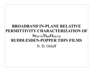
  • 1. BROADBAND IN-PLANE RELATIVE PERMITTIVITY CHARACTERIZATION OF Sr(n+1)Ti(n)O(3n+1) RUDDLESDEN-POPPER THIN FILMS N. D. Orloff
  • 2. This is for Jaclyn, and my Mom, and Dad.
  • 3. The Story 1. The Setup. 2. The Theory (C. Fennie) 3. The Materials (D. Schlom) 4. The Measurements
  • 4. Frequency is Important. Electric Field tuning is good.
  • 5. Thin films enables...           
  • 6. Thin films enables...         Courtesy of D. Muller   
  • 7. Sr n+1Ti nO3 n+1/DyScO3/DyScO3(110) Sr n+1Ti nO3 n+1 (110) Ba(1-x)= 5 (x)TiO3 700 Sr n = 5 700 K11(in−plane) at 300 K K11(in−plane) at 300 K n 600 600 n=6 n=6 500 n=4 500 n = 4 400 n = 3 11 400 n = 3 K 300 300 200 200 Im(K11) 100 n = 2 ~ 100 n = 2 0 0 0 05 5 10 10 15 15 20 2 Frequency (GHz) (GHz) Frequency Dispersion means loss.
  • 8. The Figure of Merit? Multiple Reports & Materials! 200 1 (0) − (V) “FOM” = Figure of Merit tan δ (0) 150 Figure of Merit “FOM” = Q · %Tuning 100 50 0 0 40 80 120 160 200 240 280 320 Temperature [K] Temperature (K)
  • 9. The Figure of Merit? 200 1 (0) − (V) “FOM” = Figure of Merit tan δ (0) 150 Figure of Merit “FOM” = Q · %Tuning 100 50 BSTO ~ 30 0 0 40 80 120 160 200 240 280 320 Temperature [K] Temperature (K) Bigger FOM is better.
  • 10. What is strain?            Lattice mismatch = Strain.
  • 11. Strained STO is awesome!  Peak is Critical Temperature. 
  • 12. Strained STO is awesome!  Tunability is huge.
  • 13. Strained STO is awesome?   Losses are terrible. 
  • 14. Craig Fennie has a great idea. SrTiO3 is the n = ∞ member of a group of materials…
  • 16. A simpler picture...                       
  • 17. How does ferroelectricity emerge as a function of series number?
  • 18. Theory predicts that…. Courtesy of T. Birol 0.0% LSAT 1.0% DyScO3 1.7% GdScO3 they should be ferroelectric.
  • 19. Darrell Schlom says,                        I can grow that with MBE.
  • 20. How does ferroelectricity emerge as a function of strain?
  • 21. Successful growth of RPs!                       
  • 22. # of Peaks is      like n...                  
  • 23. These are going to be really really hard to measure.      
  • 24.                 
  • 25.                 
  • 26. We can’t use these at HF... 20 0.1mm Bad 0.325mm Capacitance [pF] 15 0.875mm 1.835mm 2.9mm 10 5 0 6 7 8 10 10 10 Frequency [Hz] they show distributed effects.
  • 27.                    
  • 28.                    iω t0 −γ· iω t1 Vo e Vo e e
  • 29. Propagation Constant (γ) at 300 K 50 180 DyScO3 GHz ) −1 40 Sr7Ti6O19(n = 6) 150 Re[γ](m ) −1 30 120 −1 Im[γ / f ](m 20 90 10 60 0 7 8 9 10 11 10 10 10 10 10 Frequency (Hz)
  • 30. The effect of the film is really small. So...
  • 31. A new metrology approach.                                               
  • 32. What it sort of looks like.                 
  • 33. The Copper Chuck...                         40 mm        
  • 34. We measure this...                    for each test wafer.
  • 35. Sr n+1Ti nO3 n+1 2500 Tc 50 nm/DyScO3(110) #1 1 MHz 25 nm/GdScO3(110) #1 2000 K11(in−plane) 1500 1000 n=5 n=4 500 n=3 n=2 0 0 50 100 150 200 250 300 350 400 Temperature (K)
  • 36. Sr n+1Ti nO3 n+1 400 Critical Temperature (K) DyScO3 #1 350 DyScO3 #2 300 DyScO3 #3 GdScO3 #1 250 200 150 100 50 1 MHz 0 n=2 n=3 n=4 n=5 n=6 n=∞ Series Number ( n)
  • 37.            +V -V     
  • 38. Sr7Ti6O19 (n = 6)/DyScO3(110) T = 120K T = 180K K11(in−plane) at 1 MHz 600 800 400 600 400 200 700 1000 T = 240K (Tc) T = 300K 600 800 500 600 400 400 −50 0 50 −50 0 50 Electric Field (kV/cm)
  • 39. tan(δ11)(in−plane) at 300 K Sr n+1Ti nO3 n+1 DyScO3 #3 1 MHz GdScO3 #1 0.02 0.01 0 n=2n=3n=4n=5 n=6 Series Number (n)
  • 40. Sr n+1Ti nO3 n+1/DyScO3/DyScO3(110) Sr n+1Ti nO3 n+1 (110) Ba(1-x)= 5 (x)TiO3 700 Sr n = 5 700 K11(in−plane) at 300 K K11(in−plane) at 300 K n 600 600 n=6 n=6 500 n=4 500 n = 4 400 n = 3 400 n = 3 300 300 200 200 FOM = 60 FOM = 2 100 n = 2 ~ 100 n = 2 0 0 0 05 5 10 10 15 15 20 2 Frequency (GHz) (GHz) Frequency We don’t want to see this.
  • 41. We measure this...                    for each test wafer.
  • 42. Sr n+1Ti nO3 n+1/DyScO3(110) 700 n=6 K11(in−plane) at 300 K 600 n = 5 500 n = 4 400 n = 3 300 200 100 n=2 0 0 1 2 3 4 5 6 7 8 9 10 11 10 10 10 10 10 10 10 10 10 10 10 10 Frequency (Hz)
  • 43. Sr7Ti6O19 (n = 6)/DyScO3(110) 1500 Tc = 240K 1250 K11(in−plane) T = 180K 1000 T = 120K T = 60K 750 T = 300K 500 250 0 0 1 2 3 4 5 6 7 8 9 10 11 10 10 10 10 10 10 10 10 10 10 10 10 Frequency (Hz)
  • 44. Sr7Ti6O19 (n = 6)/DyScO3(110) 150 Im( K11)(in−plane) Tc = 240K 100 50 T = 300K 0 T = 120K −50 0 1 2 3 4 5 6 7 8 9 10 11 10 10 10 10 10 10 10 10 10 10 10 10 Frequency (Hz)
  • 45.            V   V      
  • 46. Figure of Merit at 300K Sr n+1Ti nO3 n+1 300 6 GHz to 7 GHz Grey Lines are 250 Min FOM to Max FOM 200 150 100 50 0 n=3 n=4 n=5 n=6 Series Number ( n)
  • 47. Summing it all up. Developed new on-wafer              metrology. 10 Hz to 40 GHz                                   1st observation of ferroelectric Sr7Ti6O19 (n = 6)/DyScO3(110) T = 120K T = 180K K11(in−plane) at 1 MHz 600 800 400 600 400 RPs (n ≠ ∞). 200 700 1000 T = 240K (Tc) T = 300K 600 800 500 600 400 400 −50 0 50 −50 0 50 Electric Field (kV/cm) Sr n+1Ti nO3 n+1 Strain, and Layering can be 400 Critical Temperature (K) DyScO3 #1 350 DyScO3 #2 300 DyScO3 #3 GdScO3 #1 250 used to control Tc. 200 150 100 50 1 MHz 0 n=2 n=3 n=4 n=5 n=6 n=∞ Series Number ( n) Sr n+1Ti nO3 n+1 Figure of Merit of 140 (n = 6) at Figure of Merit at 300K 300 6 GHz to 7 GHz Grey Lines are 250 Min FOM to Max FOM 200 300 K between 6 GHz and 150 100 50 7 GHz 0 n=3 n=4 n=5 n=6 Series Number ( n)
  • 48. Prof. D. I. & S. N. Orloff, L. Kaiser, J. Kaiser, Dr. M. & R. Wilson, J. & B. Kaiser, S. & R. London, R. & B. Hoffman, Drs. J. & D. Doran, M. & L. Schriber, M. & M. Orloff, M. & D. Lizmi, E. & S. Dennis, M. Dennis, J. Dennis, F. Orloff, C. J. & J. Long, Dr. E. Engelson, Dr. J. K. Hall, B. Smith, W. Young, A. Gretes, M. Hanlon, J. Mays, J. Kanner, L. Kirn, Dr. J. Miller, Mr. C. & A. McCann, Dr. M. R. Clary, B. Christy, Dr. C. Stark, Dr. K. Gustofson, Dr. R. Artuso, Dr. P. Redl, Prof. B. R. Conrad, Prof. J. Mateu, Dr. S. K. Dutta, Prof. J. R. Simpson, Dr. S. Hemmady, Dr. D. Mercia, Prof. S. C. Lee, Prof. A. Lewandowski, Prof. J. R. Dorfmann, Prof. C. Collado, Mr. E. Rocas, X. Li, Y. Wang, A. Haddock, Dr. S. R. Lee, Dr. S. L. Clement, Dr. D. Gu, Dr. G. C. Hilton, J. A. Beall, Dr. F. Altomare, Dr. P. Dresselhaus, Dr. Y. Xu, Dr. T. M. Wallis, Dr. P. Kabos, L. Vale, Dr. J. Higgins, Dr. M. Janezic, Dr. D. F. Williams, D. Walker, R. Ginley, L. DeSalvo, Dr. D. Schmadel, Dr. G. Jenkins Dr. M. Kelley, S. Rivera, T. Gleason, L. O'Hara, B. Kozlowski, J. Hessing, R. Monkfort, N. K. Morris, Prof. T. Cohen, Prof. S. Wallace, Prof. N. Chant, Prof. H. D. Drew, Prof. J. Goodman, Prof. S. Kamba, Prof. S. Stemmer, Prof. C. J. Fennie, T. Birol, C. H. Lee, Prof. I. Appelbaum, Prof. R. M. Briber, Prof. J. R. Anderson, Prof. S. M. Anlage, Prof. D. G. Schlom, Prof. I. Takeuchi, and Dr. J. C. Booth. I profoundly thank J. P. King for his support during the course of this work and Prof. D. I. Orloff for his critical review of this dissertation. Most of all, I thank my soon to be wife, J. R. Dennis.
  • 49. Thanks to my advisors...
  • 50. And the rest of the...