1. Dual Tree Kernel Conditional Density Estimation
NP Slagle and Alexander Gray
February 2012
1 Introduction
1.1 Estimation of Densities
Density estimation, an approach to prediction, is ubiq-
uitous across most scientific and engineering disci-
plines. Conditional density estimation, in which we es-
timate P(Y1, ..., YDY
|X1, ..., XDX
) given a random vec-
tor (Y1, ...YDY
, X1, ..., XDX
), can capture salient re-
lationships between features not obvious when esti-
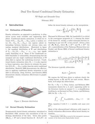
mating marginal distributions. Illustrated in figure
1, the marginal distribution of Y and distributions
of Y1, ..., YDY
|X1, ..., XDX
= x1, ..., xDX
vary signifi-
cantly depending on x. Many of the conditionals ex-
hibit bimodality or unimodality, demonstrating that the
marginal and any single conditional distribution of Y
often fails to capture the underlying structure. Condi-
tional density estimation when DY = 1 is also superior
to linear regression, since therein we estimate the quan-
tity E(Y1|X1, ..., XDX
) rather than the entire conditional
distribution. Budavari 2009 demonstrates the effective-
ness in applying conditional density estimation to red
shift in astronomy. Song, Gretton, and Guestrin 20XX
demonstrate density estimation effectiveness in graphi-
cal models.
Figure 1: Bivariate distribution
1.2 Kernel Density Estimation
Nonparametric kernel density estimation, introduced in
Rosenblatt 1956, assumes only smoothness of the un-
derlying distribution of the data. Given data points
{Xi}N
i=1 ⊂ Rd and a kernel function K : R/to/R+, we
define the kernel density estimate as the interpolation
ˆfh(x) =
N
i=1
1
hdN
K


x − Xi
h

 (1)
Discussed in Silverman 1986, the bandwidth h is critical
to the convergence properties of 1, whereas the choice
of the kernel K, usually a radial unimodal function in-
tegrating to one over Rd, is less crucial1. Given a data
set {Xi, Yi}N
i=1 where Xi ∈ RDX and Yi ∈ RDY for
all i, a generalization of the Nadaraya-Watson form (see
Gooijer and Zerom 2003) of kernel conditional density
estimation is
ˆfa,b,c(y|x) =
N
i=1
1
aDY bDX N
K

 y−Yi
a

K

 x−Xi
b


N
i=1
1
cDX N
K

 x−Xi
c


(2)
The literature typically abbreviates
Kh(t) =
1
hd
K(t/h) (3)
We express the full form above to indicate clearly the
scaling factors, as Xi and Yi are each vectors. Hence-
forth, we’ll adopt the abbreviation.
For DY = DX = 1, Chen, Linton, and Robinson 2001
summarizes choices for a, b, and c appearing earlier in
the literature; herein we assume b = c, a simplification
resulting in, as discussed in Chen, Linton, and Robinson
2001 for DY = DX = 1,
∞
−∞
. . .
∞
−∞
ˆfa,b,b(s|x)ds1 . . . dsDY
= 1 (4)
Thus, equation 2 with b = c satisfies unit mass over
RDY .
Many of the aforementioned references with respect to
density estimation effectiveness affirm kernel density es-
timation.
1
Epanechnikov 1969 offers a proof of the asymptotic minimum
variance of the finite-extent Epanechnikov kernel.
1

2. 1.3 Bandwidth Selection
Conventional bandwidth selection2 approaches for
KCDE include maximization of the log-likelihood func-
tion, and likelihood cross validation (LCV), minimiza-
tion of the least-squares cross validation estimate, or
least-squares cross validation (LSCV). Bandwidth selec-
tion using LCV, formulated as
LCV (a, b) = argmaxa,b
N
i=1
log ˆfa,b,b(yi|xi) (5)
typically suffers high sensitivity to outliers (Silverman
1986.) The LSCV, discussed in Hansen 2004, attempts
to minimize the integrated square error (ISE)
ISE(a, b) = . . . (f(y|x) − ˆfa,b,b(y|x))2
f(x)dydx
(6)
with a score approximation of
LSCV (a, b) =
1
N
N
i=1
Hi − 2Ii (7)
where
Hi =
j=i k=i Kb( xi − xj )Kb( xi − xk )Jj,k
j=i k=i Kb( xi − xj )Kb( xi − xk )
(8)
Jj,k = . . . Ka( y − yj )Ka( y − yk )dy (9)
and
Ii =
j=i Kb( xi − xj )Ka( yi − yj )
j=i Kb( xi − xj )
(10)
As discussed in Hansen 2004, if K is the Gaussian kernel,
then 9 reduces to
Jj,k = Ka
√
2( yj − yk ) (11)
Since computing the LSCV requires O(N3) time, we cal-
culate bandwidths for larger N assuming that there ex-
ist ca, pa, cb, pb such that a∗ = caNpa and b∗ = cbNpb .
Hansen 2004 and Silverman 1986 offer precedents in the
literature, and our empirical studies indicate that log-
linear regression offers a reasonable approximation.
2
Chen, Linton, and Robinson 2001 offer a survey of bandwidth
selection choices for various cases of parameters a, b, and c where
DX = DY = 1.
For finite extent kernels (such as spherical and Epanech-
nikov), the LSCV can be problematic, as the denomi-
nator and numerator of some terms in the summation
can be zero. To mitigate this, we observe that given a
weighted sum over nonzero weights S({αi, ωi(t)}n
i=1) =
n
i=1 αiωi(t)
n
i=1 ωi(t)
such that limt→0 ωi(t) = 0 for all i and
such that for all i, j ∈ {1, ..., n}, limt→0
ωi(t)
ωj(t) = ∞,
1, or 0, then given {ωi1 (t), ...ωik
(t)} that produce ∞
limits in numerators the most frequently, we have
limt→0 S({αi, ωi(t)}n
i=1) = 1
k
k
j=1 αij . Less formally,
the sum approaches the arithmetic mean of the com-
ponents whose weights approach zero the most slowly.
Since our kernel functions over various point pairs serve
as weight functions akin to the ω functions, we can apply
this technique when calculating LSCV over the finite-
extent kernels. Also, we can apply this approach to
infinite-extent kernels since they exhibit numerical im-
precision on smaller bandwidths.
1.4 Tree Methods for Kernel Density Esti-
mation
Gray 2000 introduces an efficient algorithm for kernel
density estimation that organizes both the reference and
query sets into space-partitioning trees (ball trees or kd-
trees) such that coordinates over each node are maxi-
mally tight. Figure 1.4 shows leaf nodes of a kd tree
applied to a bivariate distribution. Gray’s dual tree al-
gorithm recurses on the query and reference trees to ap-
proximate upper and lower bounds on each pq, the mass
of query point xq ∈ Q, pruning subtrees with a rule guar-
anteeing that the relative error between the bounds is
less than or equal to a user-specified . For each xq ∈ Q,
the estimate of pq is ˆpq =
ˆpmax
q +ˆpmin
q
2 with
ˆpq−pq
pq
≤ .
The algorithm appears in figure 3.
2

3. Figure 2: Bivariate distribution partition: The ellipses
represent covariance matrices; the large dots indicate
centroid locations and cluster masses.
DualTree(Q, T)
dl = NT Kh(δmax
QT )
du = NT (Kh(δmin
QT ) − 1)
if Kh(δmin
QT ) − Kh(δmax
QT ) ≤ 2
N ˆpmin
Q
then
for all xq ∈ Q do
ˆpmax
q + = dl, ˆpmin
q + = du
end for
ˆpmin
Q + = dl, ˆpmax
Q + = du
return
else
if leaf(Q) and leaf(T) then
DualTreeBase(Q,T)
return
else
DualTree(Q.left,closer-of(Q.left,{T.left,T.right}))
DualTree(Q.left,farther-of(Q.left,{T.left,T.right}))
DualTree(Q.right,closer-of(Q.right,{T.left,T.right}))
DualTree(Q.right,farther-of(Q.right,{T.left,T.right}))
end if
end if
DualTreeBase(Q, T)
for all xq ∈ Q do
for all xt ∈ T do
ˆpmin
q + = Kh( xq − xt ), ˆpmax
q + = Kh( xq − xt )
end for
ˆpmax
q − = NT
end for
ˆpmin
Q = minq∈Q ˆpmin
q , ˆpmax
Q = maxq∈Q ˆpmax
q
Figure 3: Gray and Moore’s dual tree algorithm
1.5 Related Work
Early efforts to reduce time complexity in kernel den-
sity estimation include Scott 1992 and Fan 1994, apply-
ing univariate methods to the multivariate case. Gray
and Moore 2000, stated earlier, introduces efficient tree
methods applicable to various machine learning tech-
niques, including kernel density estimation. Gray 2003
and Gray and Moore 2003 build on tree methods for
N-body problems and kernel density estimation, respec-
tively. Holmes, Gray, and Isbell 2010 applies the dual
tree approach to log-likelihood kernel conditional density
estimation for bandwidth selection, assuming DY = 1.
1.6 New Approach
In this paper, we introduce a fast algorithm for kernel
conditional density estimation based on Gray’s dual tree
approach. Heretofore, we believe this is the fastest ker-
nel conditional density estimation algorithm for predic-
tion. The generalized algorithm presented herein allows
for arbitrary DY and DX, extending the univariate case
in both the label and conditioning variable.
2 Our Approach
2.1 Dual Tree for KCDE
Based on equation 2, we can apply the dual tree
algorithm to both the numerator and denominator
summations, then simply perform a pointwise divi-
sion over the query set. Naively, we can build four
trees, one query/reference pair for the set of attributes
Y1, ..., YDY
, X1, ..., XDX
and one query/reference pair for
the conditional attributes X1, ..., XDX
. Performing a
modification (the approximation of the numerator re-
quires calculating the product of kernel functions, evi-
dent in equation 2; the minimum and maximum bounds
between nodes requires filtering on both the set of con-
ditional attributes and its complement) of the dual tree
algorithm on each of the two pair of trees gives esti-
mates for the numerators and denominators of query
point masses. However, applying in both the numer-
ator and denominator dual tree approximations fails to
give an error rate in the quotients. Fortunately, we can
leverage algebra to obtain component-wise error bounds.
Lemma 1. Let > 0, n > 0, and d > 0. If ˆn−n
n ≤
α = 2+ and
ˆd−d
d ≤ β = 3+ , then
ˆn
ˆd
−n
d
n
d
≤ .
Proof. We can transform the hypothesized inequalities to
1 −
2 +
n ≤ ˆn ≤ 1 +
2 +
n (12)
and
1 −
3 +
d ≤ ˆd ≤ 1 +
3 +
d (13)
The desired inequality is
(1 − )
n
d
≤
ˆn
ˆd
≤ (1 + )
n
d
(14)
3

4. Inverting equation 13, then combining equations 12 and 13, we have


1 − 2+
1 + 3+


n
d
≤
ˆn
ˆd
≤


1 + 2+
1 − 3+


n
d
(15)
Clearing and simplifying the bounds in equation 15, we have
6 + 2
6 + 7 + 2 2
n
d
≤
ˆn
ˆd
≤
6 + 8 + 2 2
6 + 3
n
d
(16)
For the upper bound, note that since 0 < + 2
,
6 + 8 + 2
2
< +
2
+ 6 + 8 + 2
2
= (1 + )(6 + 3 ) (17)
Thus, we have
6 + 8 + 2 2
6 + 3
< 1 + (18)
The lower bound follows similarly.
Theorem 1. Applying error bounds from 1, applying
the dual tree algorithm to both the numerators and de-
nominators of the query set evaluations specified in equa-
tion 2 gives relative error for each query point xq ∈ Q.
We can eliminate much of the memory footprint of our
approach by generating a single tree for each of the query
and reference sets, calculating upper and lower bounds
on both the numerators and denominators simultane-
ously. If we reach our stopping criterion for either the
numerator or denominator, but not both, we can simply
filter our remaining recursion on the set failing to meet
its respective criterion. We can share efforts further
in that the maximum and minimum pairwise node dis-
tances along the conditioning attributes appear in both
the numerator and denominator calculations. Key to
the algorithm is the observation that the maximum and
minimum distances between nodes are greedily selected
in kd-trees, preserving optima not just in a single mono-
tonic kernel expression but in the product of kernels.
Unfortunately, ball trees fail to share this property; how-
ever, a slight adjustment in selecting the maximum and
minimum distances over conditioning attributes solves
this minor issue. We present the shared algorithm in
figure 4.
3 Empirical Study3
3.1 Data Sets
We apply the KCDE algorithm to selections from the
Sloan Digital Sky Survey (SDSS) DR64. Unless stated
3
To determine optimal bandwidths, we apply the LSCV on data
sets of smaller sizes of N (under 1K), performing a uniform search
over [0.0001, 10]×[0.0001, 10]; we obtain optimal bandwidth pairs,
then calculate ca, cb, pa, pb where (a∗
, b∗
) = (caNpa
, cbNpb ). With
these formulas, we estimate optimal bandwidths for larger values
of N.
4
The first two features are x and y location coordinates of ce-
lestial objects; subsequent features are visual attributes.
DualTreeKCDE(Q, T, yContinue, xContinue)
dlY = NT Ka(δmax
y,QT )Kb(δmax
x,QT )
duY = NT (Ka(δmin
y,QT )Kb(δmin
x,QT ) − 1)
dlX = NT Kb(δmax
x,QT ), duX = NT (Kb(δmin
x,QT ) − 1)
if yContinue and Ka(δmin
y,QT ) − Ka(δmax
y,QT ) ≤ 2α
N ˆpmin
y,Q
then
for all yq ∈ Q do
ˆpmax
y,q + = dlY , ˆpmin
y,q + = duY
end for
ˆpmin
y,Q + = dlY , ˆpmax
y,Q + = duY , yContinue = false
end if
if xContinue and Kb(δmin
x,QT ) − Kb(δmax
x,QT ) ≤ 2β
N ˆpmin
x,Q
then
for all xq ∈ Q do
ˆpmax
x,q + = dlX , ˆpmin
x,q + = duX
end for
ˆpmin
x,Q + = dlX , ˆpmax
x,Q + = duX , xContinue = false
end if
if not yContinue and not xContinue then
return
else
if leaf(Q) and leaf(T) then
DualTreeBaseKCDE(Q,T,xContinue,yContinue)
return
else
DualTreeKCDE(Q.left,closer-of(Q.left,{T.left,T.right}),
xContinue, yContinue)
DualTreeKCDE(Q.left,farther-of(Q.left,{T.left,T.right}),
xContinue, yContinue)
DualTreeKCDE(Q.right,closer-
of(Q.right,{T.left,T.right}), xContinue, yContinue)
DualTreeKCDE(Q.right,farther-
of(Q.right,{T.left,T.right}), xContinue, yContinue)
end if
end if
DualTreeBaseKCDE(Q, T, xContinue, yContinue)
if yContinue then
for all yq ∈ Q do
for all yt ∈ T do
ˆpmin
y,q + = Ka( yq − yt )Kb( xq − xt ), ˆpmax
y,q + =
Ka( yq − yt )Kb( xq − xt )
end for
ˆpmax
y,q − = NT
end for
ˆpmin
y,Q = minq∈Q ˆpmin
y,q , ˆpmax
y,Q = maxq∈Q ˆpmax
y,q
end if
if xContinue then
for all xq ∈ Q do
for all xt ∈ T do
ˆpmin
x,q + = Kb( xq − xt ), ˆpmax
x,q + = Kb( xq − xt )
end for
ˆpmax
x,q − = NT
end for
ˆpmin
x,Q = minq∈Q ˆpmin
x,q , ˆpmax
x,Q = maxq∈Q ˆpmax
x,q
end if
Figure 4: Shared Dual Tree for KCDE
4

5. otherwise, we apply the Epanechnikov kernel and sphere
the data (subtract empirical feature means and scale by
empirical standard deviations). We also apply shared
dual tree to the MiniBooNE particle data set (see Frank
and Asuncion 2010).
3.2 Scaling with Data Set Size
Table 1 exhibits run times using optimal bandwidths
on various sizes of data taken from SDSS DR6 with
DX = DY = 1. Empirically, the shared dual tree algo-
rithm requires a decaying fraction of the time required
to execute the naive summation.
Shared Dual Tree on SDSS, DX = DY = 1
N Shared Dual Tree Naive a∗
b∗
1K 0.089355 1.037543 0.00814 0.0004765
10K 2.299951 102.464691 0.00663 0.000227
100K 72.103015 10246.469* 0.0054 0.000108
1M 1885.179322 1024647* 0.00439 5.156e-5
10M 99699.903932 102464691* 0.003578 2.4567e-5
Table 1: Shared Dual Tree on SDSS, DX = DY = 1
3.3 Scaling by Bandwidths
Over various data sets, values of N, and kernels, ex-
ecution times with shared dual tree exhibit a similar
pattern over the bandwidth pair a, b. Figure 5 exhibits
this pattern. Notice that optimal runtimes occur when
either both bandwidths are large (greater than 10) or
either bandwidth is quite small (less than 0.1.) Band-
widths exhibiting suboptimal runtimes lie along the two
crested regions along each bandwidth axis. The optimal
bandwidth rests between the crested intersection and the
origin, somewhat on the downward slope. The crested
region seems to coincide with naive time complexity, and
the pattern persists with higher N.
Figure 5: Execution Times Per Bandwidth, N = 100,
DX = DY = 1
3.4 Scaling by Dimension
Table 2 exhibits run times over various values of DX.
Shared Dual Tree on MiniBooNE, DY = 1, N = 100, 000
DX Shared Dual Tree Naive a∗
b∗
4 4650 20500* 4.3e-7 0.17
8 ??? 41000* 3e-8 0.25
16 3500 82000* 2.2e-9 0.32
Table 2: Shared Dual Tree on MiniBooNe, DY = 1, N =
100, 000
3.5 Kernel Choice
Comparisons between the spherical, Epanechnikov, and
Gaussian kernels across selections from SDSS DR6 ap-
pear in table 3. Notice, as expected, that the Gaussian
kernel requires the most time, roughly 50% more than
that of the Epanechnikov. The spherical kernel, as ex-
pected, offers the fastest computation time.
Kernels Using Shared Dual Tree on SDSS, DX = DY = 1
N Spherical Epanechnikov Gaussian
1K 0.070923 0.089355 0.128079
10K 2.240860 2.299951 3.313672
100K 71.934361 72.103015 104.501412
Table 3: Shared Dual Tree with Various Kernels on
SDSS, DX = DY = 1
5

6. 4 Conclusions
The shared dual tree algorithm offers significant speed-
up over the naive computation when bandwidths a and
b are sufficiently small or sufficiently large. Building
on a series of dual tree approaches to density estima-
tion (Gray and Moore 2003, Holmes, Gray, Isbell 2010),
shared dual tree extends the framework to compute ker-
nel conditional density estimates with an approximation
guarantee and an approach in cases in which the weights
are zero.
5 References
1. T. Budavari. A Unified Framework for Photometric Red-
shifts. The Astrophysical Journal, Volume 695, Issue 1, 747-
754, 2009.
2. X. Chen, O. Linton, P.M. Robinson. The Estimation
of Conditional Densities, unpublished discussion paper,
No.EM/01/415, 2001.
3. V.A. Epanechnikov. Non-parametric estimation of a mul-
tivariate probability density. Theory of Probability and its
Applications 14, 153158, 1969.
4. J. Fan and J. Marron. Fast Implementations of Nonparamet-
ric Curve Estimators. Journal of Computational and Graph-
ical Statistics, 3:35-56, 1994.
5. A. Frank and A. Asuncion. UCI Machine Learning Repos-
itory [http://archive.ics.uci.edu/ml]. Irvine, CA: University
of California, School of Information and Computer Science,
2010.
6. J.G.D. Gooijer and D. Zerom, On conditional density esti-
mation. Statistica Neerlandica 57 (2), 159176, 2003.
7. A.G. Gray and A.W. Moore. N-Body Problems in Statistical
Learning. T.K. Leen, T.G. Dietterich, and V. Tresp, editors,
Advances in Information Processing Systems 13 (December
2000). MIT Press, 2001.
8. A.G. Gray and A. W. Moore. Rapid Evaluation of Multiple
Density Models. In Artificial Intelligence and Statistics 2003,
2003.
9. B.E. Hansen. Nonparametric conditional den-
sity estimation, unpublished manuscript. URL:
http://www.economics.ucr.edu/seminars/fall04/ Bruce-
Hansen.pdf, 2004.
10. M.P. Holmes, A.G. Gray, and C.L. Isbell Jr. Fast Kernel Con-
ditional Density Estimation: A Dual Tree Monte Carlo Ap-
proach. Computational Statistics and Data Analysis, 1707-
1718, 2010.
11. M. Rosenblatt. Remarks on some nonparametric estimates
of a density function. Annals of Mathematical Statistics 27:
832837, 1956.
12. D.W. Scott. Multivariate Density Estimation. Wiley, 1992.
13. B.W. Silverman. Density Estimation for Statistics and Data
Analysis, Chapman and Hall/CRC, 1986.
14. L. Song, A. Gretton, C. Guestrin. Nonparametric Tree
Graphical Models via Kernel Embeddings. 765-772, 20XX.
6