The Object Detection Capabilities of the Bathymetry Systems Utilised for the 2015 Common Dataset
•
3 likes•1,602 views


Recommended
Recommended
More Related Content
What's hot
What's hot (20)
Similar to The Object Detection Capabilities of the Bathymetry Systems Utilised for the 2015 Common Dataset
Similar to The Object Detection Capabilities of the Bathymetry Systems Utilised for the 2015 Common Dataset (20)
The Object Detection Capabilities of the Bathymetry Systems Utilised for the 2015 Common Dataset
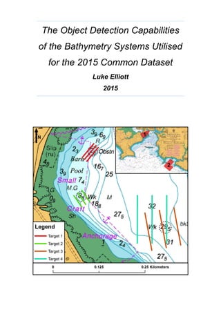
- 1. The Object Detection Capabilities of the Bathymetry Systems Utilised for the 2015 Common Dataset Luke Elliott 2015
- 2. ~ i ~ THE OBJECT DETECTION CAPABILITIES OF THE BATHYMETRY SYSTEMS UTILISED FOR THE 2015 COMMON DATASET by LUKE SCOTT ELLIOTT Thesis submitted to Plymouth University in partial fulfilment of the requirements for the degree of MSc HYDROGRAPHY PLYMOUTH UNIVERSITY FACULTY OF SCIENCE & ENGINEERING In collaboration with The United Kingdom Hydrographic Office September 2015 Journal Format
- 3. ~ ii ~ This copy of the thesis has been supplied on condition that anyone who consults it is understood to recognise that its copyright rests with the author and that no quotation from the thesis and no information derived from it may be published without the author’s prior written consent. Masters Dissertation Licence This material has been deposited in the Plymouth University Learning and Teaching repository under the terms of the student contract between the students and the Faculty of Science and Technology. The Material may be used for internal use only to support learning and teaching. Materials will not be published outside of the University and any breaches of the licence will be dealt with following the appropriate University policies.
- 4. ~ iii ~ DISSERTATION CONTENTS Dissertation........................................................................................................1 Dissertation Appendices ..................................................................................35 Journal of Coastal Research (JCR) Editorial Policy ...............35 JCR Full Author Instructions ..................................................38 2m Cube................................................................................48 Caris Workflow ......................................................................50 Beam Footprint Calculations..................................................52 Actual Line Plans ...................................................................54 Line Statistics ........................................................................57 Target images........................................................................65
- 5. ~ iv ~ This dissertation is in the format of a scientific paper laid out to the specification set by The Journal of Coastal Research. It should be noted that there is no specified word count or page limit for this journal apart from the abstract, <250 words. Additional images and supplementary notes are indicated by superscripted numbers throughout the report (e.g. 1, 2, 3… ). A list of these can be found in Appendix i at the end of the paper. For the paper copy only, supplementary documents, key tables from spreadsheets and relevant images have been appended to the paper. Separate documents and full spreadsheets of workings are available in electronic form only.
- 6. ~ 1 ~ The Target Detection Capabilities of the Bathymetry Systems Utilised for the 2015 Common Dataset Short Running Head: 2015 Common Dataset Comparisons Luke S. Elliott School of Marine Science & Engineering Plymouth University Plymouth, Devon PL4 8AA, UK Tel. +44 7876 484046 E-Mail. luke.s.elliott@outlook.com E-M . luke.elliott@ukho.gov.uk
- 7. ~ 2 ~ ABSTRACT A key element of Shallow Survey 2015 was the collection of a common dataset by manufacturers of bathymetry systems. Following on from a paper by Andrew Talbot comparing the systems utilised in the 2005 Common Dataset (Talbot, 2006), this paper provides analysis of all systems used to comprise the 2015 dataset. The key theme of the paper is the Target Detection Task (TDT), a new element to this year’s common dataset. The task was implemented to test the object detection capabilities of the systems. The paper proves that all systems that took part in the Common dataset have the ability to pass IHO Order 1a standard and the LINZ equivalent specification. It was found that many of the manufacturers failed to complete the set line plan over the four targets whilst adhering to the Common Dataset Specification. Thus it was not possible to complete a like for like comparison between systems. Therefore, any judgement made on systems based on this paper should take into account all line statistics completed. These along with other supplementary information, indicated by superscripted numbers throughout the paper and noted in Appendix i can be supplied by the author upon request. Suggestions are provided for future datasets. Additional index words: Hydrography, Shallow Survey, Object Detection, Swath Systems, IHO, LINZ
- 8. ~ 3 ~ INTRODUCTION Shallow Survey was established in 1999, in Sydney, Australia and is the international conference for hydrographic surveys in shallow water. The fundamental aim of the conference series is to promote progress in survey techniques within the coastal zone. The terms ‘shallow water’ and ‘coastal zone’ can be relatively subjective. In terms of the conference, the former is considered to be areas with depths less than 200m. The area incorporating the shore out to the continental shelf; usually 100 – 200 miles from the shoreline, is deemed the coastal zone (Inman & Brush, 1973). Of the many topics covered at the conference, considerable emphasis is given to The Common Dataset (CDS). This paper builds on the ‘Shallow Survey 2005 Common Dataset Comparisons’, (Talbot, 2006). The techniques in the 2006 paper were used to assess the target detection capability of current systems on the market. The Common Dataset The CDS allows manufacturers relevant to shallow water surveying to test equipment against market competitors over the same area. This is not limited to but includes conventional echo-sounding and remote sensing techniques to acquire bathymetry, backscatter and water column data. Sub-bottom profilers, side scan sonars and laser scanners, amongst other equipment, have featured in previous datasets. The key theme behind the CDS is to allow those within the hydrographic community to make comparisons between the latest survey technologies. Thus enabling judgement to be made upon the various approaches employed by manufacturers to the many elements of shallow water surveying. The surveys are completed close to the location of the conference. Areas selected must be dynamic with varying depth and seabed types in order to fully test the capability of each system. The 2015 dataset was collected in Plymouth Sound and included a specific Target Detection Task (TDT). Target detection is an essential requirement of hydrographic surveys (Yang, et al., 2009). Its importance is primarily objects that pose a threat to the safe passage of shipping (Hammerstad, 2005). The aim of the TDT is to be able to analyse a systems capability to detect an object and is the focus of this paper. In this task
- 9. ~ 4 ~ manufacturers were limited by a precise specification to ensure a fair comparison between datasets. As well as the designated target area, the Royal Navy were given the chance to lay inert mine-like objects within the area unknown to the manufacturers; to further test the systems under their optimum settings. Unfortunately due to time and weather constraints, not all companies completed Area Two (Figure 1), where these objects were laid. Thus it is not an element within this review. Four manufactures; Edgetech; Kongsberg; Teledyne Reson; and WASSP, took part in the TDT in Plymouth Sound during July and August 2014 using one of three vessels. Following the survey period Kongsberg returned in March 2015 using a fourth vessel to test two more systems to be included in the dataset. A specification was provided to companies taking part. Three tasks were set; Area 1, 2 and the TDT (located within Area 1) (Figure 1). The TDT consisted of four conspicuous targets in the Barn Pool Area; remains of a WWII loading jetty used during the D-Day landings 1; two ammunition barges; and a 2m cube laid for the previous 2005 CDS 2 . Strict line plans were set, consisting of three lines for each target with the following criteria: 140° swath coverage sector (±70° from nadir); 6kt speed over ground (SOG); North to South orientation with an offline tolerance of 5m 3 . The data collected during the TDT was used in this paper to analyse the Target detection capability of each individual system. Many of the companies supplied processed datasets with different levels of cleaning as well as the raw data. Only the raw data was used within this review to ensure a non-biased analysis of the unprocessed data. Cleaning is a standard procedure with all bathymetric data, to remove any noise in the water column. However the cleaning process tends to be subjective, hence the unprocessed datasets are used here to allow each system an unbiased chance of detecting the target. This said, tide and sound velocity profile (SVP) data was applied as necessary in order to bring the data into the software.
- 10. ~ 5 ~ Bathymetry Systems The systems that took part in the TDT are listed as follows and described below in Table 1. Edgetech 6205 Kongsberg EM2040DRX Kongsberg GeoSwath 500kHz Kongsberg GeoSwath 250kHz Kongsberg Mesotech M3 Teledyne Odom Hydrographic MB1 Teledyne Reson SeaBat 7125 Teledyne Reson SeaBat T20P WASSP WMB3250 Unlike the 2005 CDS where only one vessel was used, four vessels were used in the 2015 CDS. Each with various positioning and motion reference systems for positional aiding, reducing the commonality between the datasets. However, this was seen as the most practical way to get the most manufacturers involved in the data collection. Figure 1. TDT within Task Area 1, Plymouth Sound. The location chart (top-right) shows Areas 1 and 2 within the Sound. Both are overlaid on Admiralty Chart 1967 (ADMIRALTY Nautical Products & Services, 2012). Later, lines are referred to in relation to this orientation.
- 11. ~ 6 ~ Until recently swath bathymetry systems have been split into two distinct groups: Multibeam Echosounders (MBES) using beamforming; and Phase Measuring Bathymetric Sonars (PMBS) that use interferometric techniques. MBES measure the range for a set of angles and PMBS measure the angle for each set of ranges (Rice, et al., 2015). Both of which have clear advantages and disadvantages. MBES collect clean accurate data across the entire swath, although the resolution decreases with increased swath angle. MBES are however limited to a swath width up to ≈170° (±85 from nadir, 0°) and can provide only low resolution backscatter imagery. PMBS maintain resolution across a much wider swath and produce high resolution georeferenced sidescan imagery. However, they tend to produce noisy datasets with a blind spot directly below the unit, otherwise known as the nadir gap, as is inherent of sidescan sonars. Table 1. The manufactures and systems that completed the TDT for the dataset. Manufacturer System Release Date Cost*1 Technology*2 Bottom Detection Method*3 Max. Frequency No. of Beams Max. Swath Angle Edgetech 6205 2014 Medium MPES P 550kHz N/A 200° Kongsberg*4 EM2040DRX 2009 High MBES A, P 400kHz 512*5 200° Kongsberg GeoSwath GeoSwath Plus 250kHz 2015 Low PMBS P 250kHz N/A 240° Kongsberg GeoSwath GeoSwath Plus 500kHz 2013 Low PMBS P 500kHz N/A 240° Kongsberg Mesotech M3 2014 Low MBES A, P 500kHz 256 120° Teledyne Odom Hydrographic MB1 2012 Low MBES A, P 220kHz 512 120° Teledyne RESON SeaBat 7125 2007 High MBES A, P 400kHz 512 165° Teledyne RESON SeaBat T20P 2013 Medium MBES A, P 400kHz 512 165° WASSP WMB3250 2013 Low MBES A, P 160kHz 224 120° *1 Cost: Low Cost £0-50,000; Medium Cost £50-100,000; High Cost £100,000+ *2 MPES (Multiphase Echosounder), MBES (Multibeam Echosounder), PMBS (Phase Measuring Bathymetric Sonar) *3 Bottom Detection Method: A = Amplitude; P = Phase. Primary is given first. *4 There were two datasets analysed for the Kongsberg EM2040DRX; one completed in single swath mode and one in dual swath mode. *5 512 actual beams but the system can acquire 800/1600 depths per ping in Single Swath and Dual Swath modes respectively. This is because the system creates soft beams by analysing the phase signal of the return and thus increases the data density.
- 12. ~ 7 ~ The Multiphase echosounder (MPES) is Edgetech’s hybrid approach. Using a sidescan transmit geometry with an increased number of staves allows the primarily interferometric system to utilise MBES techniques (beamforming and beamsteering). The transmit geometry maintains the wide swath and resolution inherent of PMBS as the beamsteering capability reduces noise within the data and removes the nadir gap. The Kongsberg EM2040DRX is a configuration of the EM2040 with a single transmitter (tx) and two receivers (rx). The EM2040 tx can operate in single or dual swath mode. Dual swath mode is a method of stacking pings, i.e., 2 pings per beam, giving the ability to double the data density. 512 beams are produced per ping but each rx can obtain 800 depth solutions meaning up to 1600 measurements per swath for this configuration. The additional 288 depths are acquired by creating soft beams through analysis of the phase return in the signal. Amplitude and phase detection algorithms are used for bottom detection (Hammerstad, 2005). MBES systems use both algorithms where PMBS tend to use only the latter. On a flat seabed, amplitude detection is best suited to inner beams; those close to and at nadir, where the number of samples is small and the backscatter amplitude is highest. Moving away from the inner beams, the backscatter amplitude decreases and the number of samples becomes much greater. Therefore amplitude detection methods have poor performance within the outer beams due to the blurred returned signal. As the angle is increased the time series of the beams becomes long enough for robust phase detection so these algorithms are utilised in off-nadir beams. Amplitude detections can be used in the outer beams when a steep slope, wreck or boulder is present. These features tend to give a higher return due to a change in reflectivity, and thus amplitude detection is more appropriate (Artilheiro, 1998). IHO and LINZ Specifications The International Hydrographic Organisation (IHO) defines feature detection as ‘The ability of a system to detect features of a defined size’ (International Hydrographic Organisation, 2008). The IHO S-44 Standards specify ‘the size of features which, for safety of navigation, should be detected during the survey’. A
- 13. ~ 8 ~ feature is any object, natural or man-made, protruding from the seabed that could cause a danger to surface navigation. The standards provide specifications as to achieve specific Survey Classifications: Special Order; Order 1a; 1b; 2. In order to achieve Order 1a, cubic features less than 2 metres should be detected in depths up to 40 metres and features 10% of the depth if deeper than 40 metres (International Hydrographic Organisation, 2008). It fails however to define what a detection is. Land Information New Zealand (LINZ) created a specification that many other authorities have adopted, defining a detection as a minimum of three along track and three across track strikes on a target of specified size (2m, for Order 1a) (Land Information New Zealand, 2010). The 2m cube in the TDT is used to assess whether a system meets the IHO Order 1a standard and LINZ equivalent specification. METHODS Each manufacturer supplied datasets in a variety of formats. For the purpose of this study, full density unprocessed (raw) datasets were used for analysis. All datasets were analysed within Caris HIPS and SIPS software 4 . Supplied tide files and sound velocity profiles (SVPs) were applied to the datasets as necessary. Two GeoSwath Plus systems were used in the CDS (500kHz and 250kHz). Unfortunately the 250kHz system data was provided in a format currently unreadable in Caris software and was therefore removed from the study. From this point onwards GeoSwath refers to the 500kHz system unless otherwise stated. Unprocessed datasets were chosen in order to give each model an unbiased potential of getting a maximum number of detections on each target and avoid the aforementioned subjectivity of data cleaning. This was suited to the MBES and MPES systems with little outliers. The interferometric GeoSwath system required basic processing to remove apparent noise and errors within the data in order to make the targets suitable for analysis. Only bathymetric data was used for this comparison; some systems were also used to collect backscatter and/or water column data, analysis of which was beyond the scope of the review.
- 14. ~ 9 ~ Some manufacturers included additional lines to those set in the line plan. In the majority of cases these were removed from the study and only those adhering to the line plan were analysed. Lines that didn’t follow the specification have been highlighted but not removed from the study 5, 6, 7, 8. Figure 2 shows each of the four targets. Analysis of Target 1 was focussed on a target in the water column. Due to the stringent algorithms used by many manufacturers, mid water objects can be mistaken for noise or not picked up at all. One of the girders is horizontal in the water column and is the object analysed in this section. Accurate dimensions of the barges, Target 2 and 3, were unavailable making it impossible to complete a like for like comparison for number of hits on the target. Therefore to avoid any bias caused by subjectivity these targets were analysed qualitatively. Target 4 has known dimensions of 2m (L) x 2m (W) x 2m (H) and was used to analyse whether systems could achieve IHO Order 1a standard and the more stringent widely accepted LINZ specification. Total hits on target were examined along with along-track and across-track analysis. Figure 2. Example subset images for each of the four targets. In order to maintain coherence throughout the analysis, a shapefile was created for each of the four targets as a guide for creating each subset. For Targets 1 and 4, points were then selected to gain a value of hits on target. This makes the 1 2 3 4
- 15. ~ 10 ~ values subjective to opinion and should this test be repeated, subtle differences could appear in the values. Comparisons were made irrespective of the actual depth and position of targets. Thus removing elements external to the individual systems such as tide and meteorological effect from the analysis. Each set of images supplementary to the paper are screenshots of subsets that have the same point size, colour scale and exaggeration. Subsets of equal dimensions for each set were taken at the same view scale within Caris Subset Editor. Target 1 and 4 have a 2D point cloud image for each line completed by each system. A particular angle was selected for the 3D images of Target 1, 2 and 3 that best showed that target. Plan view surfaces created for Target 4 all have the default sun illumination of 45° azimuth and 45° elevation and 1x exaggeration applied. These measures were employed to ensure fair comparisons between systems. Aside from the data analysis, the spatial resolution of the MBES systems were also calculated at various depths using the following formulae 9 . Along-track Footprint (AtFp) (m) 𝐴𝑡𝐹𝑝 = 2 × (𝑆𝐿𝑅(tan 𝜑 2 )) (1) Across-track Footprint (AcFp) (m) 𝐴𝑐𝐹𝑝 = (tan(𝛽 + ( 𝜑 2 )) × 𝑧) − (tan(𝛽 + ( 𝜑 2 )) × 𝑧) (2) Where, SLR (Slant Range) = 𝑧 cos 𝛽 , 𝜑 = beamwidth, 𝛽 = swath angle, z = depth Figure 3 illustrates the elements used in the formulae. The first assumes a flat seabed and uses the fore-aft beamwidth stated by the manufacturer. The second can only be applied to MBES as it is a function of the port-starboard beamwidth. Beam steering is used by the MBES systems with flat transducers. This causes across-track beamwidth to change with swath angle. When a beam is steered it will use a shorter apparent portion of the receiver array therefore increasing the beamwidth by a function of the steering angle as follows:
- 16. ~ 11 ~ 𝑆𝐵𝑊 = 1 cos 𝛽 × 𝜑 (3) Where, SBW = Steered Beamwidth Figure 3. Calculating the dimensions of A. along track and B. across track beam footprint. Both diagrams are focused on a portside outer beam (Galway, 2000) The across-track formula provided by Galway (2000) has been adapted to take the above formula into account. The across-track resolution for systems using phase detection methods, is a function of bandwidth ( 1 𝑃𝑊 ) (PW = Pulse Width) not beamwidth. Hence it does not feature within the calculations. Furthermore many other factors aside of beamwidth or bandwidth govern the actual resolution (Galway, 2000), these are discussed later. RESULTS Abidance to the CDS Specification Manufacturers were expected to complete 12 lines (3 per target) with a maximum offline distance of 5m. Lines were to be completed in a North-South direction at 6kt. Plymouth Sound is a complex body of water with a series of tidal streams and a large tidal range. This makes achieving a constant speed difficult, so for the purpose of this study manufacturers were given a leeway of 5kt or more. The reason for no upper limit is that slower speeds tend to be advantageous to the quality of bathymetric swath systems, whereas higher speeds tend to result in a lower quality. They were also asked to keep a swath angle of 140° (±70° either side of nadir). Unfortunately three of the systems: M3; MB1; and WMB3250 could Depth(z) φ SLR Beam Footprint Port Starboard β B Depth(z) φ SLR Beam Footprint Bow Stern A
- 17. ~ 12 ~ achieve only 120° (±60° either side of nadir) and thus could not fully abide by the specification. All manufacturers apart from WASSP completed the set line plan over each target but the majority did so with a maximum offline distance greater than the 5m specified (Table 2). Actual line plans are available 10 . It was noted that the observed maximum tolerances were in the extremities of the lines and not over the targets themselves, so no lines were rejected from the analysis on the basis of offline tolerance. Table 2. Abiding by the specification for the TDT. Red values indicate where companies have not adhered to the specification. Model Lines Completed Line Speed (5+kt) N-S Orientation Maximum Off- line Distance (m) 6205 12/12 11/12 10/12 4.78 EM2040DRX Dual Swath 12/12 12/12 12/12 7.76 EM2040DRX Single Swath 12/12 6/12 12/12 11.54 GeoSwath Plus 500kHz 12/12 3/12 6/12 6.49 Mesotech M3 12/12 3/12 7/12 7.03 MB1 12/12 3/12 12/12 5.73 Seabat 7125 12/12 5/12 12/12 5.72 Seabat T20P 12/12 3/12 12/12 4.93 WMB3250 9/12 9/9 12/12 2.17 Line speed was taken from Caris and converted from ms-1 to knots to match the specification, only one system: EM2040DRX (Dual Swath Mode) completed all lines within the speed tolerance. WASSP also completed lines within the tolerance and had the lowest maximum offline distance, but due to time restraint only completed nine of the twelve lines. Over half of the lines were completed at slower speeds. Some companies failed to submit all lines in a North-South orientation or requested that South-North orientated lines were analysed. Many additional lines were submitted by the manufacturers. Where possible, only those abiding by the CDS specification were used 11, 12, 13, 14 . Unfortunately the swath angle value could not be displayed in Caris, in which case it is assumed that
- 18. ~ 13 ~ manufacturers followed the specification for the swath width (provided the system was capable of a 140° swath). Target 1 11, 15 The GeoSwath system had the most hits on the horizontal girder in both the port and centre lines. However, it was the only system to require cleaning in order to define the structure (Figure 4). In the square area used to take each sample almost 18% of points were removed from the GeoSwath dataset. The M3 system did particularly well in both the centre and starboard lines and the MB1 had similar values to the Seabat 7125 in the port and centre lines with considerably more hits in the starboard line. The EM2040DRX failed to pick up the girder in either single or dual-swath mode in the centre line as did the 6205 in the starboard line. The WMB3250 failed to pick up the girder in any of the lines (Figure 5). Figure 4. Highlighting the noise levels in the GeoSwath dataset. A. Raw, unprocessed dataset B. Dataset with noise removed. Both diagrams are orientated in the same way. Figure 5. Number of hits on the horizontal steel girder in the water column per line for each system. 64 99 0 120 0 236 25 0 157 901 791 365 223 673 864 465 483 871 422 437 344 357 281 229 0 0 0 0 100 200 300 400 500 600 700 800 900 1000 P OR T CE N T R E ST AR B OAR D NUMBEROFHITSONTARGET LINE 6205 EM2040D Dual Swath EM2040D Single Swath GeoSwath Plus 500kHz M3 MB1 Seabat 7125 Seabat T20P WMB3250 A B
- 19. ~ 14 ~ Target 2 12, 16 The Target is charted at 8.8m depth. All systems detected the ammunition barge in all lines, with varying detail, noise levels and definition. Figure 6 gives an example of the analysed images. Table 3 provides visual based results of each system over Target 2, no quantitative data was used for this table. Figure 6. Target 2 as depicted in the centre line by the T20P 16 . Table 3. Visual results of Target 2. Model Port Centre Starboard 6205 Boundaries of barge picked up, lacks detail, cargo hold missed, sparse point density Boundaries picked up, no detail Defined boundaries, cargo hold defined, sparse point density EM2040DRX Dual Swath Well defined, good detail, high point density Well defined, cargo hold not as defined as outer lines, good detail, high point density Well defined, good detail, high point density, only system to clearly define the rear of the barge in this line (holes) EM2040DRX Single Swath As above with lower point density As above with lower point density As above with lower point density GeoSwath Plus 500kHz Well defined apart from South corner, good detail, high point density Barge appears as areas of noise in data, no boundaries Well defined boundaries, cargo hold detailed, noisy M3 Clear definition of dimensions, sparse point density, cargo hold picked up but quite noisy Clear definition of dimensions, sparse point density, cargo hold less defined than port line Barge picked up, shape/ boundaries not well defined, sparse point density MB1 Barge picked up but lacks shape and detail, very noisy Boundaries of barge picked up, lacks detail, cargo hold missed, sparse point density Barge picked up, shape/ boundaries not well defined, sparse point density Seabat 7125 Well defined, good detail. high point density, only system to clearly define the rear of the barge in this line (holes) Well defined, cargo hold not as defined as outer lines, good detail, high point density Well defined, more noise than previous lines (West side), high point density Seabat T20P Starboard side appears noisy, the rest is well defined Well defined, cargo hold not as defined as outer lines, good detail, high point density Well defined, more noise than previous lines (West side), high point density, cargo hold not as defined WMB3250 Boundaries picked up, lacks quality, very noisy, sparse point density Boundaries defined, lacks quality, sparse point density Only East boundary picked up, noisy dataset, sparse point density
- 20. ~ 15 ~ Target 3 13, 17 The Target is charted at 29.5m depth, far deeper than the first barge. All systems got hits on Target 3 in at least one line. However due to the increased depth, compared with Target 2, many of the systems failed to produce clear visualisation. In reality if this was an unknown target it wouldn’t necessarily be detected. Figure 7 gives examples of the analysed images. Like Target 2, no quantitative data was used in the analysis of this Target. Figure 7. Target 3 as depicted in the port line by A. EM2040DRX (Dual Swath Mode), B. WMB3250 17 In the port line comparison the EM2040DRX (both modes), 7125 and T20P give the most detailed image with clearly defined boundaries and little noise. The EM2040DRX in dual swath mode has a higher point density than the other two. The GeoSwath and 6205 systems have picked up the barge but without the definition of the other systems. The 6205 has a lower point density. The M3, MB1 and WMB3250 failed to produce a detailed representation of the barge. In the centre line the GeoSwath failed to detect the barge. The 6205 and MB1 found it but without clearly defined boundaries or detail. The EM2040DRX (both modes), M3, 7125 and T20P found the barge and provided a little detail of the cargo hold but boundaries are not quite as sharp as before. Due to time constraints WASSP did not supply a centre line for this target. The starboard line gave very similar results to the port line. The EM2040DRX in dual swath mode had the highest point density and similar definition to the 7125. The T20P appears with slightly more noise than the previous line. The GeoSwath system has a greater definition in this line but appears noisy. The 6205 has a defined boundary but lacks detail due to the sparse point density. The M3, MB1 and WMB3250 failed to clearly detect the barge. A B
- 21. ~ 16 ~ Target 4 14, 18 Seven of the nine systems clearly ‘detected’ an object at the known location of the 2m cube. The 6205 shows a small patch of noise in the correct location but would appear not substantive enough to be picked up as a target by a data processor. The GeoSwath surface is the noisiest dataset but it shows an object is present in the correct area (Figure 8). Edgetech 6205 Kongsberg EM2040DRX Dual Swath Kongsberg EM2040DRX Single Swath Kongsberg GeoSwath Plus 500kHz Kongsberg Mesotech M3 Teledyne Odom MB1 Teledyne Reson Seabat 7125 Teledyne Reson Seabat T20P WASSP WMB3250 Figure 8. A shoal depth true position surface of all three lines for each system. Each square represents an area 33 x 30m at 1m resolution. Six of the nine systems got hits on target on every completed line (Figure 9), thus passing IHO order 1a (Table 4). WASSP only had time to collect data for the centre line. The MB1 failed to detect the cube in the port or starboard lines. The 6205 did not detect the cube in the port and centre lines. The M3 did not detect the cube in the starboard line.
- 22. ~ 17 ~ Figure 9. Number of hits on the cube per line for each system. The highest number of hits on target was by the M3 in the centre line followed by the EM2040DRX in dual swath mode in the same line and the EM2040DRX in single swath mode in the port line (Figure 9). In all but two cases a system that passed the IHO feature detection for Order 1a, also passed the equivalent more stringent LINZ specification. The M3 and GeoSwath systems each had a line; port and centre respectively that detected the cube thus passing the IHO Order 1a standard, but did not meet the requirements of the LINZ specification (Table 4). Table 4. Whether or not the systems passed the IHO Order 1a and LINZ specification. Port Line Centre Line Starboard Line IHO LINZ IHO LINZ IHO LINZ 6205 No No No No Yes Yes EM2040DRX Dual Swath Yes Yes Yes Yes Yes Yes EM2040DRX Single Swath Yes Yes Yes Yes Yes Yes GeoSwath Plus 500kHz Yes Yes Yes No Yes Yes M3 Yes No Yes Yes No No MB1 No No Yes Yes No No Seabat 7125 Yes Yes Yes Yes Yes Yes Seabat T20P Yes Yes Yes Yes Yes Yes WMB3250 Yes Yes 0 0 13 38 145 60 131 66 30 70 8 39 1 200 0 0 20 0 34 37 33 78 42 42 0 20 0 0 50 100 150 200 P OR T CE N T R E ST AR B OAR D NUMBEROFHITSONTARGET LINE 6205 EM2040D Dual Swath EM2040D Single Swath GeoSwath Plus 500kHz M3 MB1 Seabat 7125 Seabat T20P WMB3250
- 23. ~ 18 ~ As previously mentioned many manufacturers supplied additional lines. Figure 10 shows that the 6205 can detect the cube despite not appearing substantially in the set line plan. Table 5 provides statistics proving that the line passes the feature detection specifications for both IHO Order 1a and the LINZ equivalent. Full statistics for all lines are available 11, 12, 13, and 14 Figure 10. An additional line completed by Edgetech, A. detection of the cube by the 6205, B. location of the additional line. P = Port, C = Centre and S = Starboard. The square is the 33x30m area used to take all samples of Target 4. Table 5. Line statistics taken for the additional 6205 line. Totalnumberof hitsontarget Numberofalong- trackhitson target(Profiles) Max.Numberof across-trackhits ontarget(Beams) Min.Numberof across-trackhits ontarget(Beams) Averagespeedof line(kt) Heading(°) SwathWidth(m) HeightofTarget (m) WidthofTarget (m) PingRate (pulse/sec) Additional Line (6205) 54 9 11 1 5.17 163.55 140 2.0 4.8 10.18 DISCUSSION Beam footprint is a measure of a systems resolution. For MBES the footprint is heavily influenced by the beamwidth. The appended spreadsheet is based upon the specified nadir beamwidths provided by the manufacturers (See Appendix i) 9 . A smaller footprint results in a higher resolution. All footprints increase with depth as beams spread further; hence limiting the swath angle in the specification to attempt to achieve an unbiased comparison. However the footprint is influenced by the accuracy of the ship’s navigation and motion systems, water sound velocity, meteorological conditions and tide. Increased tides, i.e., springs vs neaps, will lead to an increased footprint due to a larger spread of beams leading to a lesser resolution. The GeoSwath 250kHz (removed from the A B A P C P S
- 24. ~ 19 ~ analysis) and M3 were tested together, as were the MB1 and T20P. All other systems were tested on different weeks susceptible to a variety of weather and tidal conditions. The EM2040DRX has the highest calculated resolution at all depths followed by the 7125 and T20P. The MB1 has the lowest calculated resolution throughout. These results are reflected by the indicative cost of each system provided in the introduction (Table 1). Analysing each individual line to assess whether manufacturers adhered to the specification was simply to see how feasible a like for like comparison was. Prior to analysing the lines other observations were made. Four vessels were used in the collection of the CDS, each with its own Motion Reference Unit (MRU) and Navigation system. It is difficult to complete an unbiased like for like comparison of the systems for two reasons. Firstly, datasets were collected at different times of the year under different meteorological and tidal conditions. Secondly only one company (WASSP) fully observed the specification for each completed line (Table 2). Unfortunately due to time restraint WASSP only completed 9 of the 12 lines. The critical elements of the specification are speed and swath angle. These will make a significant difference to the data quality. Operating accurately at a larger swath angle is more economical as more of the seabed is covered in a shorter period of time. Swath angle is crucial as reducing it condenses the number of beams into a smaller area giving a higher point density and often quality over the targets. This would clearly be advantageous to manufacturers. As aforementioned it wasn’t possible to analyse the swath angle within the software, therefore it is assumed that manufacturers followed the criteria. However the M3, MB1 and WMB3250 maximum achievable swath angle is 120° (±60° either side of nadir), making the criteria unachievable. It is assumed swath angle was set to the maximum 120° for these systems. Vessel speed is equally important, as slower speeds mean that more pings are covering each point on the seabed, giving a higher quality result. Over half of the completed lines were run at speeds of less than 5kt. Consequently a higher quality result for one line may be simply due to a slower speed and furthermore
- 25. ~ 20 ~ a lower quality line resulting from a higher speed that the system isn’t capable of working at. Target 1 Any or all of the girders could have been looked at within Target 1. The horizontal one was chosen to establish a system’s ability to detect objects suspended in the water column as these are commonly missed due to the bottom-track algorithms employed by manufacturers. Overall the GeoSwath system had the largest cumulative hits on target over the three lines, 2057, closely followed by the MB1 and M3 with 1819 and 1760 respectively. Interferometric technology allows a vast sampling rate, hence the GeoSwath system has the highest hits on Target. As standard filters were not applied on import to Caris, the data required manual cleaning due to the level of noise in the water column. Standard procedures would include the application of filters to avoid this need. The EM2040DRX in either dual or single swath mode failed to pick up the girder in the centre and the WMB3250 failed to detect the girder in any of the submitted lines. Port Line Taking the numbers out of the equation and referring to the images shows that hits on target alone is a poor indicator of a systems quality. In the port line, the GeoSwath, 7125 and T20P systems fully detected the horizontal girder (Figure 11). Although well defined, the GeoSwath dataset appears a little noisy compared with the 7125 and T20P. Although the GeoSwath has more than twice the hits on target, the 7125 defines the girder clearer with little noise as data points are not as spread. The MB1 got more hits on the girder than the 7125 but is difficult to see in the image due to the surrounding noise. It must be noted that the rest of the girders are not visible in the image (MB1). Although the EM2040DRX got hits on the girder, it is not well defined thus resembling noise in the water column. Considering the system works at the same frequency as the 7125 and T20P and has almost 25% more depths, it is the bottom detection algorithms, employed by Kongsberg rather than the system itself causing the lack of detection. All port line images apart from the MB1 and WMB3250 picked up at least two of the vertical girders clearly 15 .
- 26. ~ 21 ~ Figure 11. Port line as acquired by A. GeoSwath 500kHz, B. 7125, C. T20P Centre Line As a result of the condensed inner beams passing directly over the target, five of the nine systems fully detected the horizontal girder with a high level of clarity and generally less noise in the nadir line than either of the outer lines. The EM2040DRX in either mode failed to detect the horizontal girder and got less hits on the other girders than it did in the port and starboard lines. The MB1 dataset shows far less noise in the centre line and thus clearer definition on the girders but still remained noisy. The WMB3250 gives better definition on the vertical girders but nothing on the horizontal. Starboard Line Two of the systems failed to detect any of the girders in the starboard line: 6205 and WMB3250. Five of the systems detected the horizontal girder and the EM2040DRX in both single and dual swath modes detected half of it. Whether or not algorithms were adjusted through gain settings or similar is unknown. Considering the other two lines gathered by the EM2040DRX in either mode, does not show the horizontal, either settings or environmental conditions may have changed. A B C
- 27. ~ 22 ~ Target 2 and 3 Targets 2 and 3 are the remains of WWII ammunition barges but at different depths, charted at 8.8m and 29.5m respectively. The trend throughout is that the detail of Target 2 is far higher than Target 3. As depth increases, beams are more spread out, increasing the beam footprint which lowers the resolution and quality of the image. By zooming in to the images it is possible to see the difference between the along track hit spacing (known also as profiles). Spacing is a lot wider in Target 3 due to the deeper depth hence less detail in all datasets. All systems detected the barges with varying levels of detail. The general trend throughout the images of the two targets is that the more expensive systems (EM2040DRX, 7125, T20P) gave the finest detail. In three of the six lines run over the two barges however, the M3 (one of the cheaper systems) had comparable levels of detail to these systems (Figure 12). The 6205 gave good boundary definition but lacked the detail on the surface of the barges. The GeoSwath system gave good levels of detail in the outer lines but not in the centre lines. This highlights the common issue with PMBS systems of lack of coverage in the nadir region due to a blind spot directly beneath the system. Figure 12. The centre lines as collected by the M3 over A. Target 2, B. Target 3. For both targets the cheaper systems (M3, MB1, WMB3250) show extensive divergence in quality between the centre and outer lines. These systems are limited to 120° swath angle at which it is assumed was used over the targets. It is well known that MBES systems lose data quality in their outer beams due to an increased beam footprint which is highlighted with these targets especially. The more expensive systems have much smaller beam footprints throughout the swath than the cheaper systems. The GeoSwath (also a cheaper system) and B A A
- 28. ~ 23 ~ 6205 should not follow this pattern as the technology allows these systems to maintain resolution across the complete swath. Target 4 All systems detected the cube in at least one pass, proving that all systems are capable of passing IHO Order 1a (Figure 8 and Figure 9). Only four datasets got a detection on all three passes: EM2040DRX (Single/Dual Swath mode); 7125; and T20P. The GeoSwath and M3 systems each had a line that detected the object therefore passing IHO Order 1a but failed to pass the LINZ equivalent. Figure 13 shows the two lines and highlights a need for a more stringent object detection specification than the IHO Order 1a standard. The GeoSwath got 8 hits on target (Figure 13A); to pass the LINZ specification, 9 hits are required. The M3 system got only one hit on the cube in the port line giving no definition of its shape or dimensions (Figure 13B). If this wasn’t an object of known location it would possibly be removed as noise. It may however trigger the processor to analyse the backscatter (MBES) or co-registered side-scan (PMBS/MPES). This highlights the subjectivity of data cleaning and thus reiterating the fact simply ‘detecting’ a target is not a stringent enough standard. This shows the importance of survey specifications, like the one set by LINZ, specifying a detection in greater detail; for example three along track by three across track hits. Figure 13. Passing IHO Order 1a standard but not the LINZ equivalent specification. A. the centre pass completed with the GeoSwath 500kHz system, B. the port line pass for the M3 system. Analysis of the cube also reiterates the outcome of Target 1, hits on target alone is not a good measure of a system’s quality. In the port and starboard lines for instance, the GeoSwath system has the third and second highest value for hits on target respectively but fails to define the surfaces of the cube. The 7125 has B A A
- 29. ~ 24 ~ less hits than the T20P but with superior definition of the two cube surfaces detected in both the outer lines. The M3 and MB1 systems detected the cube in the centre line but not in the outer port and starboard lines. This is explained by examining the calculated beam footprints of the systems (Table 6). In order to get a reliable target detection, the beam footprint of the system must be smaller than the target being detected. It was found that the cube is at approximately 38m depth, directly below the system (at nadir, 0°) in the centre line and approximately 45° swath angle when passed in the outer lines. Table 6 shows the beam footprint at both angles for the EM2040DRX, 7125 and T20P remain below 2m hence detection of the cube in all lines. For the M3 and MB1 the beam footprint is larger than the cube at 45°; approximately where the cube was found in the swath of the outer lines, hence detections were not made. Unfortunately outer lines were not supplied for the WMB3250. Table 6. MBES Beam footprint at 38m depth (the approximate depth of the cube) at 0° (Centre Line) and 45° (Average swath angle for the appearance of the cube in the port and starboard lines). 0° 45° EM2040DRX 0.33 x 0.66 0.47 x 1.33 M3 1.99 x 1.06 2.81 x 2.12 MB1 1.99 x 2.65 2.81 x 7.53 Seabat 7125 0.66 x 0.33 0.94 x 0.94 Seabat T20P 0.66 x 0.66 0.94 x 1.88 WMB3250 2.32 x 0.36 3.28 x 1.01 This said, the M3 had the single most hits in a line, with 200in the centre line. A possible explanation for this is due to the large 3° along track beamwidth. In the nadir and inner beams, MBES tend to use only amplitude detection and thus cannot differentiate where exactly within the 3° the target is, as it measures the range for the angle series within the swath. For a strongly reflecting target, like the cube, off beam hits could also be reported as in-beam. If this hypothesis is correct, it also explains why both the M3 and MB1 show the width of the cube as 3.2m and 3.8m respectively. The T20P has a 0.5° wider across track beamwidth
- 30. ~ 25 ~ than the 7125 and thus could be the reason for it having more hits on the cube despite being the lower specification system of the two. Although the 6205 ‘detected’ the cube in the starboard line, points are only 35cm from the seabed and there is no definition of the surfaces. Regardless, the requirements for passing both the IHO Order 1a standard and LINZ equivalent specification were achieved (Figure 14). Had the cube been an unknown object, it may not have been detected making it the only one to fail the detection in all lines. However in an additional line (Figure 10), the cube was detected when approached from a different angle to the line plan. This line provided comparable definition of the top of the cube to any of the other systems. The average speed for the additional line was 0.89 - 1.43kt slower than the lines in the set line plan at 5.17kt. This could suggest that the 6205 must operate at lower speeds in order to fully comply with IHO Order 1a. Figure 14. Starboard line over the cube as run by Edgetech's 6205 system. Although hits are on the cube no definition of the cubes surfaces are apparent. An anomaly was apparent in the port lines between the single and dual swath datasets for the EM2040DRX. The single had over three times the hits than the dual swath dataset. The centre and starboard line show the dual swath mode giving approximately double the points acquired in single mode as expected given
- 31. ~ 26 ~ the technology. The anomaly could have occurred due to a change in vessel speed between lines, the line offset between the two, a difference in tide or a drastic change in environmental conditions between lines, i.e., changing currents or similar. With regards to the vessel speed, the single mode line was completed at a faster average speed putting it at a disadvantage. Over the cube, the maximum line offset between the two was 1.5m and the tide difference between completing the two lines was 0.6m both of which are negligible. Further analysis of the speed was completed for the EM2040DRX (Table 7). By measuring the average distance between pings surrounding the cube and multiplying by the ping rate for the line gives the speed the vessel was going at a specific point, as opposed to assuming the average for the line. Table 7. Further analysis for the speed of the line over the cube for the EM2040DRX. Ping rate for the dual swath is in reality double the value presented in the table. Port Ping Spacing (m) Ping Rate (pulse/sec) Speed of Line (m/s) Speed of Line (kt) Average speed of line (kt) Dual Swath 0.6 6.39 3.83 7.45 5.66 Single Swath 0.2 7.01 1.40 2.73 6.00 Centre Dual Swath 0.5 6.76 3.38 6.57 6.23 Single Swath 0.5 6.97 3.49 6.77 5.95 Starboard Dual Swath 0.6 6.40 3.84 7.46 6.06 Single Swath 0.4 6.68 2.67 5.19 5.64 It is possible to see that for the centre and starboard lines, the actual speed over the cube is within ±1.5kt of the average. The port line differs considerably more; in dual swath mode the cube was being passed 1.79kt faster than the average for the line and in single swath mode it was passed at a speed 3.27kt slower than the average line speed. Therefore the single swath port line was completed at approximately a third of the speed hence having almost triple the points on the cube in comparison to the system in dual swath mode.
- 32. ~ 27 ~ CONCLUSIONS The aim of this paper was to compare bathymetry systems currently on the market that compile the 2015 Common Dataset (CDS). A comparison of this sort is difficult to complete without subtle bias from external influences. The most unbiased method would be to use only one vessel, on one day and have a system either side of it operating concurrently. However this would limit the dataset to only two systems. The CDS has made it possible for unlimited companies to take part in a practical manner. The ideal situation would have been to have one vessel at different times through the year, this would still have natural bias with regards to tide and meteorology but greatly reduces human induced bias toward the systems. Four vessels with various motion compensation and navigation systems were used to complete the CDS meaning subtle bias will be inherent to particular systems. In reality every vessel setup is different and each bathymetry system should work to its full potential regardless, making the comparisons viable. Many companies completed the Target Detection (TDT) without meeting the criteria set out in the original specification. Some lines were completed in South to North orientation rather than the requested North to South, at speeds often considerably slower than 5kt and were often off the set line plan in excess of the allowed 5m. The required swath angle could not be adhered to by all systems and could not be examined within the software. As a result no system judgement should be made without taking into account the line statistics: heading; ping rate; average speed of line; and swath width as discussed in this paper. It would be suggested that for future CDSs to keep the orientation and line plans with the same stringency but to reduce both swath angle and survey speed to allow all systems to operate under optimum conditions. For the reasons above, a like for like comparison to determine which system is best at the various elements of the TDT is not viable. It does however provide analysis of each dataset and the conditions for which the task was carried out, allowing judgement on each system to be made. This study proves that all systems that took part have the ability to achieve IHO Order 1a standard and
- 33. ~ 28 ~ LINZ equivalent specification through analysis of Target 4; the 2m cube. This analysis emphasises the subjectivity of data cleaning and that simply ‘detecting’ a target is not a stringent enough standard. It also highlights elements of the standard/specification that could be improved. ACKNOWLEGEDGEMENTS A thanks firstly to my advisors Gwyn Jones, Tim Scott and colleague at the UKHO Andrew Talbot for their extensive advice, guidance and teaching during the writing of this paper. This paper would not have been possible without the co- operation of all manufacturers that took part in the CDS along with everyone involved in the data collection, thank you to you all. A special thanks to Lisa Brisson (Edgetech), Peter Hogarth, Craig Wallace (Kongsberg), Pim Kuus (Teledyne Reson) and Justin Kiel (WASSP), my main contacts with regards to the CDS who provided answers to the never ending series of questions. Another massive thanks goes to Nolwenn Collouard at Caris for sharing her extensive Caris knowledge in order to bring the range of various datasets into the software and provide advice when errors occurred.
- 34. ~ 29 ~ LITERATURE CITED ADMIRALTY Nautical Products & Services, 2012. Chart 1967. Taunton: United Kingdom Hydrographic Office. Scale 1:7500, 1 Sheet. Artilheiro, F. M. F., 1998. Analysis and procedures of multibeam data cleaning for bathymetric charting. 1st ed. Fredericton: Department of Geodesy and Geomatics Engineering, University of New Brunswick. Galway, R. S., 2000. Comparision of Target Detection Capabilities of the Reson Seabat 8101 and Reson Seabat 9001 Multibeam Sonars, Fredericton, New Brunswick: University of New Brunswick, Report. Hammerstad, E., 2005. Meeting the Challenges of the IHO and LINZ Special Order Object Detection Requirements. San Diego, U.S. Hydro 2005. Inman, D. L. & Brush, B. M., 1973. The Coastal Challenge. Science, 181(4094), pp. 20-32. International Hydrographic Organisation, 2008. IHO Standards for Hydrographic Surveys (Special Publication No. 44). 5th ed. Monaco: International Hydrographic Bureau. L-3 Communications SeaBeam Instruments, 2000. Multibeam Sonar Theory of Operation. 1st ed. East Walpole: L-3 Communications SeaBeam Instruments. Land Information New Zealand, 2010. Contract Specifications for Hydrographic Surveys, Version 1.2, New Zealand Hydrographic Authority. Wellington: Land Information New Zealand. Lekkerkerk, H. J. & Theijs, M. J., 2012. Handbook of Offshore Surveying: Volume I - Projects, Preperation & Processing. 2nd ed. Voorschoten: Skilltrade BV. Rice, G. et al., 2015. Chapter 5 - Acquisition: Best Practice Guide. In: X. Lurton & G. Lamarche, eds. Backscatter measurements by seafloor‐mapping sonars - Guidelines and Recommendations. s.l.:s.n., pp. 107-132. Talbot, A., 2006. Shallow Survey 2005 Common Dataset Comparisons. Hydro International, 10(1), pp. 39-51. Yang, E. et al., 2009. Small Object Detection Using SHOALS Bathymetric Lidar. Norfolk, U.S. Hydro 2009.
- 35. ~ 30 ~ TABLES Table 1. The manufactures and systems that completed the TDT for the dataset. ..........................................................................................................................6 Table 2. Abiding by the specification for the TDT. Red values indicate where companies have not adhered to the specification. ...........................................12 Table 3. Visual results of Target 2. ..................................................................14 Table 4. Whether or not the systems passed the IHO Order 1a and LINZ specification.....................................................................................................17 Table 5. Line statistics taken for the additional 6205 line. ................................18 Table 6. MBES Beam footprint at 38m depth (the approximate depth of the cube) at 0° (Centre Line) and 45° (Average swath angle for the appearance of the cube in the port and starboard lines). .......................................................................24 Table 7. Further analysis for the speed of the line over the cube for the EM2040DRX. Ping rate for the dual swath is in reality double the value presented in the table.......................................................................................................26
- 36. ~ 31 ~ FIGURES Figure 1. TDT within Task Area 1, Plymouth Sound. The location chart (top-right) shows Areas 1 and 2 within the Sound. Both are overlaid on Admiralty Chart 1967 (ADMIRALTY Nautical Products & Services, 2012). Later, lines are referred to in relation to this orientation...................................................................................5 Figure 2. Example subset images for each of the four targets. ..........................9 Figure 3. Calculating the dimensions of A. along track and B. across track beam footprint. Both diagrams are focused on a portside outer beam (Galway, 2000) ........................................................................................................................11 Figure 4. Highlighting the noise levels in the GeoSwath dataset. A. Raw, unprocessed dataset B. Dataset with noise removed. Both diagrams are orientated in the same way. .............................................................................13 Figure 5. Number of hits on the horizontal steel girder in the water column per line for each system.........................................................................................13 Figure 6. Target 2 as depicted in the centre line by the T20P 16.......................14 Figure 7. Target 3 as depicted in the port line by A. EM2040DRX (Dual Swath Mode), B. WMB3250 17 ....................................................................................15 Figure 8. A shoal depth true position surface of all three lines for each system. Each square represents an area 33 x 30m at 1m resolution. ...........................16 Figure 9. Number of hits on the cube per line for each system. .......................17 Figure 10. An additional line completed by Edgetech, A. detection of the cube by the 6205, B. location of the additional line. P = Port, C = Centre and S = Starboard. The square is the 33x30m area used to take all samples of Target 4. .............18 Figure 11. Port line as acquired by A. GeoSwath 500kHz, B. 7125, C. T20P...21 Figure 12. The centre lines as collected by the M3 over A. Target 2, B. Target 3. ........................................................................................................................22 Figure 13. Passing IHO Order 1a standard but not the LINZ equivalent specification. A. the centre pass completed with the GeoSwath 500kHz system, B. the port line pass for the M3 system. ...........................................................23 Figure 14. Starboard line over the cube as run by Edgetech's 6205 system. Although hits are on the cube no definition of the cubes surfaces are apparent. ........................................................................................................................25
- 37. ~ 32 ~ APPENDICIES Supplementary Information 1 - Target 1 – D-Day Loading Jetty This photo depicts a D-Day Loading Jetty. It is thought that the girders that comprise Target 1 are the remains of a jetty similar to this. 2 - Target 4 - 2m Cube The document provides information and photographs of Target 4, the 2m cube. The cube is a hollow, steel frame box with fibre glass sides. This was initially laid for a LiDAR trial in 2003 south of the breakwater. It was moved in 2004 for the 2005 CDS. Prior to the 2015 CDS divers were sent down to check the cube was clear of biological growth and debris. 3 - Shallow Survey 2015 CDS Specification The specification provided by the Shallow Survey Committee to the manufacturers wishing to complete the dataset. 4 - Caris Workflow The workflow used in Caris in order to complete the analysis. 5 - Edgetech Line Analysis 6 - Kongsberg Line Analysis 7 - Teledyne Line Analysis 8 - WASSP Line Analysis These four Excel workbooks provide information on rejected lines as well as personal communications with the manufacturers. If more than three lines were present in the dataset per target, additional lines were deleted based upon their orientation or through personal communication with the manufacturer prior to import to Caris.
- 38. ~ 33 ~ 9 - Beam Footprint Calculations This Excel workbook shows all workings to calculate beam footprints for each system based on beamwidths supplied by the manufacturers. Within the comparison sheet footprints have been provided for relevant angles in the TDT but also a table dedicated to where in the swath the cube was found. 10 - Actual Line Plans 10 - Line Plans - Raw Images (Folder) The Actual lines run by the manufacturers during the survey with maximum offline distance 11 - Target 1 – Statistics 12 - Target 2 – Statistics 13 - Target 3 – Statistics 14 - Target 4 – Statistics These Excel workbooks provide statistics for every line completed by each system over individual targets. Each system has its own sheet to show line statistics and all points counted as hits on target for Target 1 and 4 are also provided.
- 39. ~ 34 ~ 15 - Target 1 – Images 15 - Target 1 - Raw Images (Folder) 16 - Target 2 – Images 16 - Target 2 - Raw Images (Folder) 17 - Target 3 – Images 17 - Target 3 - Raw Images (Folder) 18 - Target 4 - Images 18 - Target 4 - Raw Images (Folder) All images provide visual comparison between the systems. As mentioned throughout this paper, line statistics; heading, ping rate, average speed of line and swath width must be taken into account when making comparisons. Target 1 Page 1 – 3D images of all lines – All images at the same orientation Pages 2 to 4 – 2D images of individual lines Target 2 Pages 1 to 3 – 3D images of individual lines – All images at the same orientation Target 3 Pages 1 to 3 – 3D plan view images of individual lines – All images at the same orientation Target 4 Page 1 – Base surfaces of all lines Pages 2 to 4 – 2D images of individual lines
- 40. ~ 35 ~ DISSERTATION APPENDICES Journal of Coastal Research (JCR) Editorial Policy (http://www.cerf-jcr.org/index.php/jcr/jcr-editorial-policy) Scope of the Journal The Journal of Coastal Research (JCR) covers all fields of coastal research [geology, biology, geomorphology, physical geography, climate, littoral oceanography, hydrography, coastal hydraulics, environmental (resource) management (law), engineering, and remote sensing] and encompasses subjects relevant to natural and engineered coastal environments (freshwater, brackish, and marine), as well as the protection (i.e. management and administration) of those resources within and adjacent to coastal zones (including large lakes) around the world. The JCR broadly focuses on coasts per se, but also embraces those coastal environments that extend some indefinite distance inland (i.e. to the edge of the coastal plain) or reach seaward beyond the outer margins of the sublittoral (neritic) zone (i.e. to the edge of the continental shelf). Consideration is also given to zones farther out to sea if processes or materials affect the coast. Editorial Policy The Journal of Coastal Research is published in English by the Coastal Education and Research Foundation, Inc. [CERF]. Submissions fall into one of the following main departments, which are included in most JCR issues: Research Papers, Technical Communications, Review Articles, Editorials, Letters to the Editor, Notes, Discussions and Replies, Meeting Reports, News and Announcements, Coastal Photographs, Honors and Awards, Book Reviews, Books Received, Dedications, and Errata (Corrigenda). There is a required, non-refundable manuscript submission fee for Research Papers, Technical Communications, Notes, and Review Articles (there is no
- 41. ~ 36 ~ submission fee for other contributions). CERF members receive a reduced submission fee of US$45 USD vs. US$65 USD for non-CERF members. This fee is required to offset third-party subscription hosting and maintenance costs associated with the online journal (www.JCRonline.org) and maintenance of the electronic Editorial Manager (PeerTrack) manuscript tracking and peer review system (http://www.editorialmanager.com/jcoastres/). Electronic submission of contributions is required; papers are no longer typeset from manual copy. When preparing a manuscript, it is essential to follow the JCR Author Instructions explicitly. The JCR Author Instructions can be downloaded from www.cerf-jcr.org. Contributions not following specifications, i.e. fail the technical check, will be returned to the author for proper JCR manuscript formatting. Please submit manuscripts for electronic manuscript tracking and processing at: http://www.editorialmanager.com/jcoastres/ It is not the responsibility of editors or peer reviewers to rewrite poorly prepared manuscripts. Manuscripts may be rejected solely on the basis of poor English usage and grammar. Authors who have difficulty writing scientific English may avail themselves of several English language editing services. Some options are listed below. CERF does not endorse any individual or agency. Professional qualifications and compensation must be discussed with the specific editing service the author chooses. Available editing services (in no particular order): http://www.editage.com http://www.journalexperts.com http://www.internationalscienceediting.com http://www.asiascienceediting.com http://www.prof-editing.com
- 42. ~ 37 ~ http://www.councilscienceeditors.org/jobbank/services.cfm http://www.alphascienceeditors.com Research papers, technical communications, notes, and review articles are peer reviewed in a timely manner by at least two referees. The referees assist the Editor-in-Chief in obtaining comments and suggestions for improvement of the manuscripts. The Editor-in-Chief is ultimately responsible for the material published in the JCR.
- 43. ~ 38 ~ JCR Full Author Instructions (http://jcronline.org/userimages/ContentEditor/1260312523013/JCR_author_instructions.pdf)
- 44. ~ 39 ~
- 45. ~ 40 ~
- 46. ~ 41 ~
- 47. ~ 42 ~
- 48. ~ 43 ~
- 49. ~ 44 ~
- 50. ~ 45 ~
- 51. ~ 46 ~
- 52. ~ 47 ~
- 53. ~ 48 ~ 2m Cube The following document is supplementary document 2 purely for the purpose of the dissertation submission. In terms of the paper, this document would be available electronically.
- 54. ~ 49 ~ 2 2m Cube The following information regarding the 2m Cube was acquired from Andrew Talbot. The 2m Cube is a hollow steel frame with fibre glass sides. It was built in 2003 for an MCA LiDAR trial. For the trial completed by Tenix LADS it was deployed south of Plymouth Breakwater. It was then moved to Barn Pool in 2004 for the CDS and has remained there ever since. Prior to the 2015 Common Dataset collection in 2014 divers were sent to inspect the cube to make sure it was clear of debris and biological growth that could affect the data collection. It was found to be clear.
- 55. ~ 50 ~ Caris Workflow The following document is supplementary document 4 purely for the purpose of the dissertation submission. In terms of the paper, this document would be available electronically.
- 56. ~ 51 ~ 4 Caris Workflow The workflow used in Caris in order to complete the analysis. If more than three lines were present per target in the dataset, additional lines were deleted based upon their orientation or through personal communication with the manufacturer prior to import to Caris. *As required Acquire/Create a vessel file Convert RAW data Import Data Apply Tide Correct for SVP* Merge Analysis
- 57. ~ 52 ~ Beam Footprint Calculations The following notes and tables are taken from supplementary Excel Workbook 9 purely for the purpose of the dissertation submission. In terms of the paper, the full workbook would be available electronically. NOTES SPREADSHEET 1. In this workbook phase measuring sonars (Edgetech 6205, Kongsberg GeoSwath Plus 500/250kHz) do not have a calculated across track footprint (resolution) as for these systems, the across track resolution is a function of bandwidth (1/Pulse Width) rather than beamwidth. Although these systems have a dedicated spreadsheet displaying along track resolution they are left out of the comparison tables as they cannot be compared like for like against the MBES systems in terms of beamwidth. 2. Maximum swath angle either side of nadir in the spreadsheets are 75°. Some systems have capabilities of greater swath angles (e.g. ±120° for the GeoSwath systems). These are not accounted for as for the Target Detection Task (TDT), it was stated that an angle of ±70° should be used. For those systems that are not capable of ±70° (M3, MB1 and WMB3250), predicted resolutions up to the maximum swath angle are given 3. Along-track resolution calculations assume a flat seabed. 4. Formulas are taken from Galway, R. S., 2000. Comparison of Target Detection Capabilities of the Reson Seabat 8101 and Reson Seabat 9001 Multibeam Sonars. Fredericton, New Brunswick: University of New Brunswick, Report, P15-18. Accessible from http://www.omg.unb.ca/omg/papers/MBSS_TermPaper.pdf 5. Beam steering is used by the MPES and MBES systems used in the study. Across- track beamwidth changes with beam angle. When a beam is steered it will use a shorter portion of the receiver array therefore increasing the nadir beamwidth (provided by manufacturer) by a function of the steering angle as follows: SBW = 1/cos(β) x φ (SBW = Steered Beam Width, β=Beam Angle, φ=beamwidth). The across-track formula provided by Galway (2000) has been adapted to take this into account.
- 58. ~ 53 ~ BEAM FOOTPRINT COMPARISONS SPREADSHEET Beamwidths as provided by the manufacturers Along Track Across Track 6205 0.5 EM2040DRX 0.5 1 GeoSwath Plus 500kHz 0.5 GeoSwath Plus 250kHz 0.75 M3 3 1.6 MB1 3 4 Seabat 7125 1 0.5 Seabat T20P 1 1 WMB3250 3.5 0.54 Nadir (0°) Kongsberg 2040D 0.09 x 0.17 0.17 x 0.35 0.26 x 0.52 0.35 x 0.70 Kongsberg M3 0.52 x 0.28 1.05 x 0.56 1.57 x 0.84 2.09 x 1.12 Teledyne Odom MB1 0.52 x 0.70 1.05 x 1.40 1.57 x 2.10 2.09 x 2.79 Teledyne Reson Seabat 7125 0.17 x 0.09 0.35 x 0.17 0.52 x 0.26 0.70 x 0.35 Teledyne Reson Seabat T20-P 0.17 x 0.17 0.35 x 0.35 0.52 x 0.52 0.70 x 0.70 WASSP WMB-3250 0.61 x 0.09 1.22 x 0.19 1.83 x 0.28 2.44 x 0.38 Half TDT Swath Angle (35°) Kongsberg 2040D 0.11 x 0.26 0.21 x 0.52 0.32 x 0.78 0.43 x 1.04 Kongsberg M3 0.64 x 0.42 1.28 x 0.83 1.92 x 1.25 2.56 x 1.66 Teledyne Odom MB1 0.64 x 1.27 1.28 x 2.54 1.92 x 3.82 2.56 x 5.09 Teledyne Reson Seabat 7125 0.21 x 0.16 0.43 x 0.32 0.64 x 0.48 0.85 x 0.64 Teledyne Reson Seabat T20-P 0.21 x 0.32 0.43 x 0.64 0.64 x 0.95 0.85 x 1.27 WASSP WMB-3250 0.75 x 0.17 1.49 x 0.34 2.24 x 0.51 2.98 x 0.69 Maximum Swath Angle for M£, MB1, WMB-3250 (60°) Kongsberg 2040D 0.17 x 0.70 0.35 x 1.40 0.52 x 2.09 0.70 x 2.79 Kongsberg M3 1.05 x 1.12 2.09 x 2.24 3.14 x 3.35 4.19 x 4.47 Teledyne Odom MB1 1.05 x 5.68 2.09 x 11.35 3.14 x 17.03 4.19 x 22.71 Teledyne Reson Seabat 7125 0.35 x 0.70 0.70 x 1.40 1.05 x 2.09 1.40 x 2.79 Teledyne Reson Seabat T20-P 0.35 x 1.40 0.70 x 2.80 1.05 x 4.19 1.40 x 5.59 WASSP WMB-3250 1.22 x 0.75 2.44 x 1.51 3.67 x 2.26 4.89 x 3.02 Full TDT Swath Angle (70°) Kongsberg 2040D 0.26 x 1.49 0.51 x 2.99 0.77 x 4.48 1.02 x 5.97 Kongsberg M3 Teledyne Odom MB1 Teledyne Reson Seabat 7125 0.51 x 2.18 1.02 x 4.37 1.53 x 6.55 2.04 x 8.74 Teledyne Reson Seabat T20-P 0.51 x 4.38 1.02 x 8.77 1.53 x 13.15 2.04 x 17.54 WASSP WMB-3250 Angle and Depth relevant to Cube detection (Target 4) Kongsberg 2040D 0.33 x 0.66 0.47 x 1.33 Kongsberg M3 1.99 x 1.06 2.81 x 2.12 Teledyne Odom MB1 1.99 x 2.65 2.81 x 7.53 Teledyne Reson Seabat 7125 0.66 x 0.33 0.94 x 0.94 Teledyne Reson Seabat T20-P 0.66 x 0.66 0.94 x 1.88 WASSP WMB-3250 2.32 x 0.36 3.28 x 1.01 45°, 38m0°, 38m 10m 20m 30m 40m 10m 20m 30m 40m 10m 20m 30m 40m 10m 20m 30m 40m
- 59. ~ 54 ~ Actual Line Plans The following document is supplementary document 10 purely for the purpose of the dissertation submission. In terms of the paper, this document and the raw .jpeg files would be available electronically.
- 60. ~ 55 ~ 10 Line Plans The Actual lines run by the manufacturers during the survey with the measured maximum offline distance presented. Edgetech 6205 Maximum Offline Distance: 4.78m All lines complete Kongsberg EM2040DRX Dual Swath Maximum Offline Distance: 7.76m All lines complete Kongsberg EM2040DRX Single Swath Maximum Offline Distance: 11.54m All lines complete Kongsberg GeoSwath 500kHz Maximum Offline Distance: 6.49m All lines complete Kongsberg Mesotech M3 Maximum Offline Distance: 7.03m All lines complete Teledyne Odom MB1 Maximum Offline Distance: 5.73m All lines complete
- 61. ~ 56 ~ Teledyne Reson Seabat 7125 SV2 FP4 Maximum Offline Distance: 5.72m All lines complete Teledyne Reson Seabat T20P FP4 Maximum Offline Distance: 4.93m All lines complete WASSP WMB3250 Maximum Offline Distance: 2.17m Three lines missed
- 62. ~ 57 ~ Line Statistics The following tables are taken from supplementary workbooks 11 – 14 purely for the purpose of the dissertation submission. In terms of the paper, the full workbooks would be available electronically. TARGET 1 Port Line Model Totalnumberof hitsontarget Averagespeed ofline(kt) Heading(°) SwathWidth (m) PingRate (pulse/sec) Heightof Horizontal(m) 6205 64 6.00 224.04 77 18.07 5.8 EM2040DRX Dual Swath 120 6.02 217.15 86 7.59 N/A EM2040DRX Single Swath 25 4.98 221.98 58 8.23 N/A GeoSwath Plus 500kHz 901 3.65 39.12 70 10.23 5.7 M3 223 3.00 43.41 41 15.99 6.0 MB1 465 3.96 222.54 47 16.64 5.8 Seabat 7125 422 3.80 209.73 75 9.50 5.9 Seabat T20P 357 3.47 219.17 74 7.95 5.8 WMB3250 0 5.91 218.62 44 9.74 N/A Centre Line Model Totalnumberof hitsontarget Averagespeedof line(kt) Heading(°) SwathWidth(m) PingRate (pulse/sec) Heightof Horizontal(m) 6205 99 5.61 38.49 77 18.07 5.8 EM2040DRX Dual Swath 0 5.80 218.74 100 6.95 N/A EM2040DRX Single Swath 0 4.90 217.06 56 7.59 N/A GeoSwath Plus 500kHz 791 4.19 218.28 59 11.87 5.7 Mesotech M3 673 2.77 221.88 40 16.01 6.0 MB1 483 3.94 219.80 49 16.61 5.9 Seabat 7125 437 3.97 222.43 77 10.58 5.8 Seabat T20P 281 3.39 218.62 76 6.70 5.9 WMB3250 0 5.77 223.02 49 9.72 N/A
- 63. ~ 58 ~ Starboard Line Model Totalnumberof hitsontarget Averagespeedof line(kt) Heading(°) SwathWidth(m) PingRate (pulse/sec) Heightof Horizontal(m) 6205 0 5.85 222.95 76 18.07 N/A EM2040DRX Dual Swath 236 5.91 220.45 111 6.25 5.8 EM2040DRX Single Swath 157 4.99 219.62 60 6.59 5.8 GeoSwath Plus 500kHz 365 3.91 39.99 58 11.89 6.3 Mesotech M3 864 3.11 44.47 45 16.01 5.9 MB1 871 3.80 212.25 51 18.48 6.0 Seabat 7125 344 3.16 220.54 104 8.08 5.9 Seabat T20P 229 3.47 197.61 107 6.80 5.9 WMB3250 0 6.39 222.64 51 8.57 N/A
- 64. ~ 59 ~ TARGET 2 Port Line Model ShoalestDepth overwreck(m) Averagespeedof line(kt) Heading(°) SwathWidth(m) PingRate (pulse/sec) 6205 8.8 6.35 145.57 66 18.07 EM2040DRX Dual Swath 8.7 5.96 141.97 51 19.57 EM2040DRX Single Swath 8.8 4.33 145.66 52 21.53 GeoSwath Plus 500kHz 8.5 3.74 322.21 95 8.02 Mesotech M3 10.6 4.08 324.93 32 15.99 MB1 7.2 3.66 147.03 37 18.44 Seabat 7125 9.5 3.03 146.32 57 16.54 Seabat T20P 9.6 3.15 147.22 55 19.35 WMB3250 11.9 5.50 144.12 33 17.82 Centre Line Model ShoalestDepth overwreck(m) Averagespeedof line(kt) Heading(°) SwathWidth(m) PingRate (pulse/sec) 6205 8.8 6.35 328.55 67 18.07 EM2040DRX Dual Swath 8.7 5.98 145.17 66 16.16 EM2040DRX Single Swath 8.6 4.45 143.05 61 20.18 GeoSwath Plus 500kHz 8.6 3.68 143.31 83 8.96 Mesotech M3 11 3.86 320.13 46 15.99 MB1 8.9 3.67 144.07 42 18.44 Seabat 7125 9.7 3.25 141.88 70 18.15 Seabat T20P 9.7 3.07 146.37 64 16.79 WMB3250 12 6.34 141.56 37 19.35
- 65. ~ 60 ~ Starboard Line Model ShoalestDepth overwreck(m) Averagespeedof line(kt) Heading(°) SwathWidth(m) PingRate (pulse/sec) 6205 9 4.49 139.34 78 18.11 EM2040DRX Dual Swath 8.8 6.00 132.05 73 17.05 EM2040DRX Single Swath 8.8 4.43 144.85 67 17.34 GeoSwath Plus 500kHz 7.9 3.22 320.88 41 23.75 Mesotech M3 10.1 4.17 159.10 51 15.99 MB1 7.5 3.70 144.01 39 25.64 Seabat 7125 9.7 3.56 140.97 78 19.07 Seabat T20P 9.6 3.31 143.77 70 15.54 WMB3250 12.8 6.54 145.67 41 15.33
- 66. ~ 61 ~ TARGET 3 Port Line Model Averagespeedof line(kt) Heading(°) SwathWidth(m) PingRate (pulse/sec) 6205 6.55 171.38 131 10.18 EM2040DRX Dual Swath 5.82 170.12 154 6.83 EM2040DRX Single Swath 5.31 169.28 153 6.89 GeoSwath Plus 500kHz 3.70 341.80 113 6.61 Mesotech M3 3.45 168.56 75 9.99 MB1 4.92 170.39 112 8.96 Seabat 7125 5.65 168.70 155 7.44 Seabat T20P 4.29 165.57 155 7.01 WMB3250 5.94 126.69 94 6.68 Centre Line Model Averagespeedof line(kt) Heading(°) SwathWidth(m) PingRate (pulse/sec) 6205 6.59 166.83 132 10.18 EM2040DRX Dual Swath 5.80 170.39 167 6.54 EM2040DRX Single Swath 5.49 169.68 167 6.60 GeoSwath Plus 500kHz 4.52 168.83 114 6.61 Mesotech M3 2.91 351.62 79 10.01 MB1 4.89 167.93 117 8.96 Seabat 7125 4.54 164.68 168 6.67 Seabat T20P 4.25 165.90 170 6.70 WMB3250 N/A
- 67. ~ 62 ~ Starboard Line Model Averagespeedof line(kt) Heading(°) SwathWidth(m) PingRate (pulse/sec) 6205 5.86 168.50 132 10.17 EM2040DRX Dual Swath 5.78 170.44 162 6.50 EM2040DRX Single Swath 5.88 169.57 161 6.74 GeoSwath Plus 500kHz 3.16 352.19 114 6.60 Mesotech M3 4.20 170.79 76 9.99 MB1 4.40 170.21 108 8.96 Seabat 7125 5.37 168.49 170 6.38 Seabat T20P 4.21 169.87 167 6.48 WMB3250 5.94 139.75 91 6.48
- 68. ~ 63 ~ TARGET 4 Port Line Totalnumberof hitsontarget Numberofalong- trackhitson target(Profiles) Max.Numberof across-trackhits ontarget(Beams) Min.Numberof across-trackhits ontarget(Beams) Averagespeedof line(kt) Heading(°) SwathWidth(m) HeightofTarget (m) WidthofTarget (m) PingRate (pulse/sec) 6205 0 0 0 0 6.24 179.69 130 N/A N/A 10.18 EM2040DRX Dual Swath 38 5 11 2 5.66 182.50 165 2.0 2.0 6.39 EM2040DRX Single Swath 131 14 16 3 6.00 182.25 157 2.0 2.0 7.01 GeoSwath Plus 500kHz 70 12 22 1 4.75 143.42 126 N/A N/A 6.06 Mesotech M3 1 1 1 1 3.00 354.40 100 N/A N/A N/A MB1 0 0 0 0 4.45 177.60 107 N/A N/A 8.96 Seabat 7125 34 4 77 4 4.49 182.99 159 2.0 1.5 6.58 Seabat T20P 78 7 12 10 3.64 177.17 144 2.5 1.7 6.70 WMB3250 N/A Centre Line Totalnumberof hitsontarget Numberofalong- trackhitson target(Profiles) Max.Numberof across-trackhits ontarget(Beams) Min.Numberof across-trackhits ontarget(Beams) Averagespeedof line(kt) Heading(°) SwathWidth(m) HeightofTarget (m) WidthofTarget (m) PingRate (pulse/sec) 6205 0 0 0 0 6.60 177.91 129 N/A N/A 10.18 EM2040DRX Dual Swath 145 9 22 7 6.23 183.39 168 2.0 2.4 6.76 EM2040DRX Single Swath 66 4 19 10 5.95 179.34 163 1.9 2.2 6.97 GeoSwath Plus 500kHz 8 5 3 1 4.64 154.14 127 N/A N/A 6.05 Mesotech M3 200 23 13 4 2.77 179.96 99 2.0 3.2 10.00 MB1 20 6 6 2 4.75 179.17 112 2.0 3.8 8.96 Seabat 7125 37 9 7 1 5.39 182.14 164 2.0 2.0 6.97 Seabat T20P 42 8 7 3 4.09 175.46 161 2.6 1.9 6.70 WMB3250 20 4 6 4 6.28 180.02 92 2.0 1.7 6.25
- 69. ~ 64 ~ Starboard Line Totalnumberof hitsontarget Numberofalong- trackhitson target(Profiles) Max.Numberof across-trackhits ontarget(Beams) Min.Numberof across-trackhits ontarget(Beams) Averagespeedof line(kt) Heading(°) SwathWidth(m) HeightofTarget (m) WidthofTarget (m) PingRate (pulse/sec) 6205 13 7 3 1 6.06 179.44 128 N/A N/A 10.17 EM2040DRX Dual Swath 60 5 17 8 6.06 181.04 175 2.0 2.0 6.40 EM2040DRX Single Swath 30 3 14 7 5.64 175.10 169 1.9 1.5 6.68 GeoSwath Plus 500kHz 39 6 14 1 4.56 191.74 124 N/A N/A 6.05 Mesotech M3 0 0 0 0 3.11 358.45 97 N/A N/A N/A MB1 0 0 0 0 4.63 180.29 115 N/A N/A 8.96 Seabat 7125 33 4 11 6 4.16 174.46 168 2.0 1.5 6.39 Seabat T20P 42 5 14 1 4.09 179.16 144 2.9 1.6 6.70 WMB3250 N/A
- 70. ~ 65 ~ Target images The following tables are taken from supplementary documents 15-18 purely for the purpose of the dissertation submission. In terms of the paper, these documents and the raw .jpeg files would be available electronically. Target 1 Page 1 – 3D images of all lines – All images at the same orientation Pages 2 to 4 – 2D images of individual lines Target 2 Pages 1 to 3 – 3D images of individual lines – All images at the same orientation Target 3 Pages 1 to 3 – 3D plan view images of individual lines – All images at the same orientation Target 4 Page 1 – Base surfaces of all lines Pages 2 to 4 – 2D images of individual lines
- 71. ~ 66 ~ Target 1 – 3D Images Edgetech 6205 Kongsberg 2040DRX – Dual Swath Kongsberg 2040DRX – Single Swath Kongsberg GeoSwath Plus 500kHz Kongsberg Mesotech M3 Teledyne Odom MB1 Teledyne Reson Seabat 7125 Teledyne Reson Seabat T20P WASSP WMB-3250
- 72. ~ 67 ~ Target 1 – Port Line Edgetech 6205 Kongsberg 2040DRX – Dual Swath Kongsberg 2040DRX – Single Swath Kongsberg GeoSwath Plus 500kHz Kongsberg Mesotech M3 Teledyne Odom MB1 Teledyne Reson Seabat 7125 Teledyne Reson Seabat T20P WASSP WMB-3250
- 73. ~ 68 ~ Target 1 – Centre Line Edgetech 6205 Kongsberg 2040DRX – Dual Swath Kongsberg 2040DRX – Single Swath Kongsberg GeoSwath Plus 500kHz Kongsberg Mesotech M3 Teledyne Odom MB1 Teledyne Reson Seabat 7125 Teledyne Reson Seabat T20P WASSP WMB-3250
- 74. ~ 69 ~ Target 1 – Starboard Line Edgetech 6205 Kongsberg 2040DRX – Dual Swath Kongsberg 2040DRX – Single Swath Kongsberg GeoSwath Plus 500kHz Kongsberg Mesotech M3 Teledyne Odom MB1 Teledyne Reson Seabat 7125 Teledyne Reson Seabat T20P WASSP WMB-3250
- 75. ~ 70 ~ Target 2 – Port Line Edgetech 6205 Kongsberg 2040DRX – Dual Swath Kongsberg 2040DRX – Single Swath Kongsberg GeoSwath Plus 500kHz Kongsberg Mesotech M3 Teledyne Odom MB1 Teledyne Reson Seabat 7125 Teledyne Reson Seabat T20P WASSP WMB-3250
- 76. ~ 71 ~ Target 2 – Centre Line Edgetech 6205 Kongsberg 2040DRX – Dual Swath Kongsberg 2040DRX – Single Swath Kongsberg GeoSwath Plus 500kHz Kongsberg Mesotech M3 Teledyne Odom MB1 Teledyne Reson Seabat 7125 Teledyne Reson Seabat T20P WASSP WMB-3250
- 77. ~ 72 ~ Target 2 – Starboard Line Edgetech 6205 Kongsberg 2040DRX – Dual Swath Kongsberg 2040DRX – Single Swath Kongsberg GeoSwath Plus 500kHz Kongsberg Mesotech M3 Teledyne Odom MB1 Teledyne Reson Seabat 7125 Teledyne Reson Seabat T20P WASSP WMB-3250
- 78. ~ 73 ~ Target 3 – Port Line Edgetech 6205 Kongsberg 2040DRX – Dual Swath Kongsberg 2040DRX – Single Swath Kongsberg GeoSwath Plus 500kHz Kongsberg Mesotech M3 Teledyne Odom MB1 Teledyne Reson Seabat 7125 Teledyne Reson Seabat T20P WASSP WMB-3250
- 79. ~ 74 ~ Target 3 – Centre Line Edgetech 6205 Kongsberg 2040DRX – Dual Swath Kongsberg 2040DRX – Single Swath Kongsberg GeoSwath Plus 500kHz Kongsberg Mesotech M3 Teledyne Odom MB1 Data Not Supplied Teledyne Reson Seabat 7125 Teledyne Reson Seabat T20P WASSP WMB-3250
- 80. ~ 75 ~ Target 3 – Starboard Line Edgetech 6205 Kongsberg 2040DRX – Dual Swath Kongsberg 2040DRX – Single Swath Kongsberg GeoSwath Plus 500kHz Kongsberg Mesotech M3 Teledyne Odom MB1 Teledyne Reson Seabat 7125 Teledyne Reson Seabat T20P WASSP WMB-3250
- 81. ~ 76 ~ Target 4 – Surfaces (All Supplied Lines) Edgetech 6205 Kongsberg 2040DRX Dual Swath Kongsberg 2040DRX Single Swath Kongsberg GeoSwath Plus 500kHz Kongsberg Mesotech M3 Teledyne Odom MB1 Teledyne Reson Seabat 7125 Teledyne Reson Seabat T20P WASSP WMB-3250
- 82. ~ 77 ~ Target 4 – Port Line Edgetech 6205 Kongsberg 2040DRX – Dual Swath Kongsberg 2040DRX – Single Swath Kongsberg GeoSwath Plus 500kHz Kongsberg Mesotech M3 Teledyne Odom MB1 Data Not Supplied Teledyne Reson Seabat 7125 Teledyne Reson Seabat T20P WASSP WMB-3250
- 83. ~ 78 ~ Target 4 – Centre Line Edgetech 6205 Kongsberg 2040DRX – Dual Swath Kongsberg 2040DRX – Single Swath Kongsberg GeoSwath Plus 500kHz Kongsberg Mesotech M3 Teledyne Odom MB1 Teledyne Reson Seabat 7125 Teledyne Reson Seabat T20P WASSP WMB-3250
- 84. ~ 79 ~ Target 4 – Starboard Line Edgetech 6205 Kongsberg 2040DRX – Dual Swath Kongsberg 2040DRX – Single Swath Kongsberg GeoSwath Plus 500kHz Kongsberg Mesotech M3 Teledyne Odom MB1 Data Not Supplied Teledyne Reson Seabat 7125 Teledyne Reson Seabat T20P WASSP WMB-3250