1. FLUID MECHANICS OF
LIQUID-LIQUID SYSTEMS
by
John Reed Richards
A dissertation submitted to the Faculty of the University of Delaware in
partial fulfillment of the requirements for the degree of Doctor of Philosophy in
Chemical Engineering
Spring 1994
c 1994 John Reed Richards
All Rights Reserved
2. FLUID MECHANICS OF
LIQUID-LIQUID SYSTEMS
by
John Reed Richards
Approved:
Michael T. Klein, Sc.D.
Chairman of the Department of Chemical Engineering
Approved:
Stuart L. Cooper, Ph.D.
Dean of the College of Engineering
Approved:
Carol E. Hoffecker, Ph.D.
Associate Provost for Graduate Studies
3. I certify that I have read this dissertation and that in my opinion it meets
the academic and professional standard required by the University as a
dissertation for the degree of Doctor of Philosophy.
Signed:
Abraham M. Lenhoff, Ph.D.
Professor in charge of dissertation
I certify that I have read this dissertation and that in my opinion it meets
the academic and professional standard required by the University as a
dissertation for the degree of Doctor of Philosophy.
Signed:
Antony N. Beris, Ph.D.
Professor in charge of dissertation
I certify that I have read this dissertation and that in my opinion it meets
the academic and professional standard required by the University as a
dissertation for the degree of Doctor of Philosophy.
Signed:
T. W. Fraser Russell, Ph.D.
Member of dissertation committee
4. I certify that I have read this dissertation and that in my opinion it meets
the academic and professional standard required by the University as a
dissertation for the degree of Doctor of Philosophy.
Signed:
Leonard W. Schwartz, Ph.D.
Member of dissertation committee
5. ACKNOWLEDGMENTS
I would like to thank my advisors, Professors A. M. Lenhoff and A. N. Beris,
for patiently providing me with invaluable advice and insight during the course of
this work. Without their constant assistance and encouragement it is improbable
that this work would have been completed. I would also like to express my grati-
tude to my committee members, Professors T. W. F. Russell and L. W. Schwartz
for their comments and suggestions.
The author expresses his sincere appreciation to Dr. J. P. Congalidis,
Dr. W. D. Smith, Jr., and Dr. T. W. Liu all of E. I. du Pont de Nemours &
Co., Inc. for friendly advice and encouragement, and for computational resources.
I would also like to recall the memory of the late Professor G. F. Scheele
of Cornell University, who served as my Master of Science advisor at Cornell, and
with whom I performed the steady jet experimental measurements.
I would also like to acknowledge useful discussions with Dr. C. W. Hirt
of Flowscience, Inc., Dr. D. B. Kothe and Dr. R. C. Mjolsness of Los Alamos
National Laboratory, and gratefully acknowledge support from a University of
Delaware Competitive Fellowship, from the National Science Foundation (grant
CBT-8657185), and from the Department of Chemical Engineering of the Univer-
sity of Delaware.
In addition, I would like to thank my many friends both at the University
of Delaware and DuPont for their help and understanding. In particular, I would
like to acknowledge Ms. A. Z. Hoover for her TEX expertise.
v
6. DEDICATION
To my wife Jean Marie Richards for her untiring and patient support and to
our wonderful children Daniel Joseph and Kathleen Mary of whom I have borrowed
quite a bit of time.
vi
17. NOMENCLATURE
a Radial interfacial distance
a∗ Dimensionless interfacial radius
a0 Initial disturbance amplitude
˜a Free surface radial perturbation
aα Surface basis vector
aα Surface reciprocal basis vector
A Area
A(z∗) Velocity function for Meister and Scheele profiles
b Radius of outer free-slip cylinder
B(z∗) Velocity function for Meister and Scheele profiles
B Vector potential
Bo Bond number
c Integration constant
Ca Capillary number
D Nozzle diameter
D Rate of deformation tensor
Ds Surface rate of deformation tensor
Dd Drop diameter
dL Outward directed normal to ∂A
dS Outward directed normal to ∂ ¯V
er Radial unit vector
ez Axial unit vector
eθ Angular unit vector
∆E∗
t Dimensionless total energy
xvii
18. xviii
F Volume of fluid function
˜F Mollified volume of fluid function
FHB Harkins-Brown correction factor
Fsv Volumetric surface force
Fr Froude number
g Gravitational force vector
gi Spatial basis vector
gi Spatial reciprocal basis vector
G Dimensionless group for Meister and Scheele profiles
h Interface thickness
H Mean curvature
H Heaviside step function
I Spatial unit tensor
Is Surface unit tensor
In(x) Modified Bessel function of the first kind of order n
J Jacobian determinant
Jn(x) Bessel function of the first kind of order n
k Disturbance wavenumber
Kn(x) Modified Bessel function of the second kind of order n
Ky Mass transfer coefficient
L Jet length
(x) Interpolation function
L1 Nozzle tip distance to tank top
L2 Nozzle tip distance to tank bottom
L3 Nozzle centerline distance to tank wall
L3 Numerical boundary distance from nozzle centerline
L4 Nozzle length
L5 Velocity profile length from nozzle tip
m Instability parameter
19. xix
n Angular wavenumber
n Interfacial unit normal pointing from phase 2 to phase 1
ˆn CSF interface unit normal pointing from fluid 1 into fluid 2
˜n CSF interface normal pointing from fluid 1 into fluid 2
ˆnw CSF wall unit normal
N Wave splitting factor
Nj Buoyancy number
Oh Ohnesorge number
p Pressure
p∗ Dimensionless pressure
∆p∗
o Dimensionless centerline pressure difference, (p∗
2o − p∗
1o)
˜p Pressure perturbation
P Stress tensor
Ps Surface stress tensor
qi Spatial coordinates
qα Surface coordinates
Q Nozzle volumetric flow rate
r Radial coordinate
r∗ Dimensionless radial coordinate
R Radius
Rc Wave splitting ratio
Rd Drop radius
R(r) Radial perturbation function
Rl Latitudinal radius of curvature
Rm Meridional radius of curvature
Ro Nozzle outer radius
R∗
o Dimensionless radius of curvature at the centerline
Re Reynolds number
s Disturbance growth rate
20. xx
s∗ Dimensionless arc length
s∗
f Total dimensionless meniscus arc length
Ss Specific surface area
t Time
ˆtw CSF wall unit tangent
T(t) Time perturbation function
u, ur Radial velocity
˜u Radial velocity perturbation
u∗ Dimensionless radial velocity
u(r) Meniscus height
u∗(r) Dimensionless meniscus height
u∗
o Dimensionless meniscus height at the centerline
up Radial particle velocity
v Velocity vector
vs Surface velocity
v, vz Axial velocity
˜v Axial velocity perturbation
v∗ Dimensionless axial velocity
¯v Nozzle average velocity
vA Axial average velocity
vI Axial interfacial velocity
vp Axial particle velocity
V Volume
¯V Bulk phase volume
Vc Volume constraint
Vd Drop volume
VJ Jetting velocity
w, vθ Angular velocity
We Weber number
21. xxi
x Spatial position vector
xs Surface position vector
Yn(x) Bessel function of the second kind of order n
z Axial coordinate
z∗ Dimensionless axial coordinate
Z(z) Axial perturbation function
Greek Letters
α ≡ kR
αHN Hirt-Nichols upwinding interpolation factor
β ≡ Rm1
γ ≡ Rm2
γ Langhaar function
δ Viscosity ratio
δj
i Kronecker delta
δ(x) Dirac delta function
∆ρ Volumetric density difference, ρ1 − ρ2
Convergence criterion
ζ Parametric arc length distance
ζ Scaled axial position
η ≡ kL3
θ Angular coordinate
θ Contact angle
Θ(θ) Angular perturbation function
κ CSF mean curvature
κ Dilatational viscosity
κs Surface dilatational viscosity
λ Disturbance wavelength
λ Integration constant
µ Shear viscosity
22. xxii
µs Surface shear viscosity
ξ Particle position at time t = 0
ρ Volumetric density
ρs Surface Density
σ Interfacial tension
σ1s Interfacial surface tension between wall and fluid 1
σ2s Interfacial surface tension between wall and fluid 2
τ Viscous stress tensor
τs Surface viscous stress tensor
φ Velocity potential
˜φ Velocity potential perturbation
Φ First Streamfunction
Ψ Second Streamfunction
ψ Angle of the tangent to the meniscus with the horizontal
ψ Streamfunction
˜ψ Streamfunction perturbation
ω Perturbation angular frequency
SOR relaxation parameter
Special Symbols
Spatial gradient operator
s Surface gradient operator
N Surface gradient normal operator
(ξ, t) Fluid property
∪ Union set operator
× Cross product operator
· Dot product operator
: Double dot product operator
† Tensor transpose
23. xxiii
Abbreviations
ABDW Anwar et al. (1982)
ADI Alternating direction implicit method
AE Addison and Elliot (1950)
BEM Boundary element method
CFD Computational fluid dynamics
CH Christiansen and Hixson (1957)
CSF Continuous surface force algorithm
DV Duda and Vrentas (1967)
FEM Finite element method
FLAIR Algorithm of Ashgriz and Poo (1991)
FLOW-3D Program of Hirt (1988)
GRP Gospodinov et al. (1979)
MAC Marker and cell method
MOM Momentum equation of Richards et al. (1993)
MS Meister and Scheele
POLYFLOW Program of Crochet (1987)
R Simulations in this work and Richards et al. (1993)
RIPPLE Program of Brackbill et al. (1992)
RS Richards and Scheele (1985)
SOLA-VOF Program of Hirt and Nichols (1981)
SOR Successive overrelaxation
VOF Volume of fluid method
YS Yu and Scheele (1975)
24. ABSTRACT
The detailed hydrodynamics of selected liquid-liquid flow systems are in-
vestigated as an initial effort to provide a firm foundation for the rational design
of liquid-liquid separation processes. The specific implementation of this objective
centers on the development of a robust and flexible code to simulate liquid-liquid
flows, including high Reynolds number ones. We have applied this code to the real-
istic simulation of aspects of the complex fluid mechanical behavior, and developed
quantitative insight into the underlying processes involved. The capabilities of the
code have been explored through investigations into the fluid mechanics of several
liquid-liquid systems, specifically liquid-liquid jet formation and breakup, and the
predictions compared to experimental data in terms of quantitative information
related to drop and jet size, shape, formation and breakup, which are important
characteristics of actual liquid-liquid extractors.
The governing continuum equations that describe complex dynamic free
surface flows are derived in detail in a rational manner, and used as the basis
for the new numerical methods needed to describe the complex free surface flows.
The Volume of Fluid (VOF) method is combined with the Continuous Surface
Force (CSF) algorithm to provide a numerically stable code capable of solving
high Reynolds numbers free surface flows. Performance of all the features of the
code is verified on an extensive set of previously solved reference problems. One
of the developments during the testing was the construction of an efficient and
robust method for solving the Young-Laplace equation describing the shape of
the meniscus in a vertical cylinder for a constrained liquid volume. The method
explicitly incorporates the constraint in the equation, transforming the two-point
boundary-value problem into an initial-value one with the constraint determining
xxiv
25. xxv
the unknown centerline height. This allows rapid determination of the solution
families, which are characterized by only centerline height and meniscus arclength.
The specific problem selected to represent the complex aspects of the fluid
mechanics of extractors is the solution of the dynamic liquid-liquid jet and associ-
ated drop formation. The steady-state region near the nozzle for the laminar flow
of a Newtonian liquid jet injected vertically into another immiscible Newtonian
liquid is investigated for various Reynolds numbers by solving the axisymmetric
transient equations of motion and continuity along with appropriate boundary con-
ditions. The analysis takes into account pressure, viscous, inertial, gravitational,
and surface tension forces, and comparison with previous experimental measure-
ments performed on a xylene/water system under conditions where all of these
forces are important, shows good agreement over the entire range of conditions
studied. Comparisons of the present numerical method with the numerical results
of previous boundary-layer methods help establish their range of validity. A new
approximate equation for the shape of the interface of the steady jet, based on an
overall momentum balance, is also developed.
The full transient from liquid-liquid jet startup to breakup into drops was
also simulated numerically. The algorithm was further refined here based on its
performance on transient problems such as the solution of the free liquid-liquid
capillary jet breakup problem. The simulation predictions cover the jet length
till breakup as well as the jet and drop shapes, often far from regular. The
comparison of the simulation results with previous experimental measurements of
jet length can be judged satisfactory, given the sensitive dependence of the results
on details of the experimental set-up that are not available. In comparison with
experiment, the results of the present numerical method show a greater sensitivity
of the jet length to the Reynolds number than the best predictions previously
available based on the linear stability analysis of the free liquid-liquid capillary jet
breakup problem. The formation of drops is investigated at low to high Reynolds
numbers before and after jet formation. The numerical simulations are compared
26. xxvi
with n-heptane/water experiments and previous simplified analyses based on drop
formation before and after jetting. The comparison of the simulation results with
previous experimental measurements of drop size can be judged satisfactory within
experimental error.
Although the program and numerical techniques developed in this disser-
tation have been used mainly to solve problems involving liquid-liquid jets and
drops, many features of more complex and general liquid-liquid contacting sys-
tems are explored in the process: free surface problems involving two immiscible
liquid phases, high Reynolds number laminar flows and complex, time-dependent
interfaces, all of which are still topics of much current research. We expect this
research to influence the way complex liquid-liquid contactors are designed in the
future, with extensions to other technologies where complex interface formation
must be addressed.
27. Chapter 1
INTRODUCTION
Laminar liquid jets possess several attractive advantages over other
types of apparatus for fundamental studies of the mechanism of gas
absorption. To obtain a valid experimental test of unsteady state
diffusion theory in a flow system, it is imperative that the fluid
dynamics of the system be known accurately.
L. E. Scriven & R. L. Pigford (1959)
Liquid-liquid systems are important to workers in many areas of engineer-
ing, physics, and chemistry. A few examples of current interest are liquid-liquid ex-
traction equipment (Treybal, 1963, 1980; Jeffreys, 1987; Rousseau, 1987, Tsouris
and Tavlarides, 1990), liquid-liquid jets (Richards et al., 1993, 1994a, 1994b),
space applications in propulsion systems, life support, and storage (Kim et al.,
1994), coating flows (Ruschak, 1985; Christodoulou and Scriven, 1989), oil-water
mixtures in pipeline flow (Joseph et al., 1984), extrusion of polymers (Mavridis
et al., 1987), secondary oil recovery (Weidner and Schwartz, 1991), interfacial
tension measurements (Li and Fu, 1992), liquid bridges (Russo and Steen, 1989;
Slobozhanin and Perales, 1993), static menisci (Finn, 1986; Cuvelier and Schulkes,
1990), and interfacial rheology (Edwards et al., 1991).
In this dissertation we seek an improved understanding of the fluid me-
chanics underlying liquid-liquid extraction, a widely used unit operation in which
solutes dissolved in a liquid solution are separated by contact with another, gen-
erally immiscible, liquid. If different solutes in the original solution distribute
themselves differently between the two phases, a certain degree of separation will
develop, and this may be enhanced by multiple contacts in staged operation. If
1
28. 2
the liquids are left in contact long enough, mass transfer between the two phases
causes the solute distribution to approach an equilibrium condition. Extractors
can be constructed in many forms, which can be run batch or continuous, e.g.,
mixer-settlers, plate columns, packed columns, as well as more exotic designs.
Many articles and books have been written on the subject, and the details of cur-
rent design techniques are well documented in, for example, Treybal (1963, 1980),
Jeffreys (1987), and Rousseau (1987).
The efficiency and stability of the separation depend on the underlying pro-
cesses taking place in the stage. These are the fluid flow field, the thermodynamic
equilibria, and the mass transfer within and between phases. The research pro-
posed here focuses on the fluid mechanics alone, as once the flow field is known,
the mass transfer and thermodynamic effects can, in principle, be added to com-
plete the analysis. The fluid mechanics of the extractor are dependent on the type
of device considered. If it is a sieve-tray extractor, the light fluid rises through
the continuous phase in trains of drops. If the extractor is a mixer-settler, the
dispersed phase is broken into drops by the energy of an impeller, with turbulent
flow commonly found in practice.
1.1 Four Distinct Levels of Analysis
Various levels of analysis can be applied to liquid-liquid extractors, de-
pending on the information sought, and can be classified as corresponding to the
discrete macroscopic (phenomenological), pseudo-continuum, continuum, or the
molecular level. Each level of analysis can be used to answer different questions
to different degrees of accuracy. Most plant design work is typically performed at
the macroscopic level, where little information is required on the internal details
of the system. Equipment design is at the pseudo-continuum level where empir-
ical information is needed to determine appropriate values of model parameters.
This dissertation is not concerned with questions at the macroscopic level such as
the ones related to the overall performance of the extractor, where most of the
29. 3
design work has occurred in the past. On the opposite end of the scales of length,
questions addressed at the molecular level are mostly concerned with the physical
properties of the components of the system and the boundary conditions, which
again are fairly well characterized. It remains to examine the extractor at the two
remaining levels.
A more detailed level of analysis than the macroscopic level, sometimes
referred to as the pseudo-continuum level, provides a more elaborate description of
the internal structure of the system and the transport within it. For example, mass
transfer coefficients are often used in equipment design (Treybal, 1980). However,
such descriptions still involve spatial averaging (e.g., over a swarm of droplets or
over random column packing) or temporal averaging (in turbulent flow), so that
quantities such as velocities and concentrations do not represent the true values
at a given point in the system. Further, the transport properties (e.g., turbulent
viscosities) are not true state properties, and their process dependence again makes
empirical information necessary.
These limitations are obviated at the continuum level, where velocities and
concentrations are local quantities and transport properties such as viscosities,
densities, surface tensions, and diffusivities, are true state variables. The obvious
problem is that most actual liquid-liquid contactors are much too complex in
their geometry and operation to permit a full continuum description, even with
the computational capabilities available today. In this dissertation, therefore, we
seek a middle ground, by analyzing at the continuum level idealized liquid-liquid
systems pertinent to actual extractors. We expect these analyses to enhance our
understanding of more realistic systems in two ways:
i. Among the systems we examine are ones that represent key elements
of one or more types of actual contactors; for example, a liquid-liquid jet is
representative of the situation above an orifice on a sieve tray.
ii. The parametric dependence of the behavior seen in the ideal model
systems is expected to be related to that in more complex systems; dimensionless
30. 4
parameters that determine the size and the specific surface area of liquid-liquid
jets and drops are investigated.
The object is to model the velocity and pressure fields as well as the interface
shape and location in a two-phase system that has one or more free surfaces.
Various simplified situations can be envisioned. The ones chosen for this work are
the liquid-liquid jet, and the drops formed before and during jetting. Two regions
are considered for the liquid-liquid jets: the steady region near the nozzle, and the
entire region from the nozzle to the breakup of the jet into drops.
1.2 Background
As noted above, most previous analysis and design work on liquid-liquid
contactors has been performed at the macroscopic or the pseudo-continuum level.
Results of such studies, and procedures based on them, may be found in, for
instance, Treybal (1963, 1980), Perry and Green (1984), Jeffreys (1987), and
Rousseau (1987). More detailed analyses at the pseudo-continuum level have
been undertaken using other approaches. For example, Guimaraes et al. (1988,
1990) used the population balance approach to model the effects of drop breakage
and coalescence on the hydrodynamics and mass transfer efficiency of liquid-
liquid continuous-flow stirred tanks at steady-state. However, even in these more
elaborate models it is necessary to estimate parameter values based on empirical
data. It is only at the continuum level, where transport properties are true state
variables, that this problem can be overcome. However, as noted earlier, the
analysis of only relatively idealized systems is possible at the continuum level, even
with the computational capabilities available today. A variety of such systems have
been studied in the past:
Isolated drops. Analytical models of single drops in idealized situations have
a long history. For example, the oscillation of a stationary drop can be described
exactly in the inviscid case (Lamb, 1932), and it has been studied more recently
for small Reynolds numbers by Lundgren and Mansour (1988). More complex
31. 5
systems have been examined either numerically or experimentally or both. Oliver
and Chung (1987) investigated the flow of a fluid sphere translating in another fluid
by solving numerically the steady-state Navier-Stokes equations inside and outside
the sphere using a streamfunction formulation. They obtained numerically the
velocity and pressure distributions inside and outside the sphere. Surface tension
acts to keep the drop spherical, but at high shear rates the drop will deform, and
eventually break. Isolated drops have been experimentally investigated during
breakup and coalescence (Clift et al., 1978; Ashgriz and Poo, 1990). The slender
body theory of Acrivos and Lo (1978) can be used for breakup at non-zero Reynolds
numbers, but requires that the drop or bubble that is breaking up must be
elongated. Stone and Leal (1989) have numerically investigated the dynamics of
drop deformation and breakup at low Reynolds numbers; Bentley and Leal (1986)
studied these effects experimentally. Basaran et al. (1989) studied small amplitude
drop oscillations in liquid-liquid systems both experimentally and theoretically
and Jeelani and Hartland (1991) investigated the collision of two oscillating liquid
drops.
Liquid-liquid jet. When one liquid is injected into another, a jet may
be formed. That this occurs in sieve plate columns has motivated its study in
apparatuses specifically designed for mass transfer and surface tension experiments
with a single jet (Skelland and Huang, 1977, 1979; Skelland and Walker, 1989).
Meister and Scheele (Meister, 1966; Meister and Scheele, 1967, 1969a, 1969b;
Scheele and Meister, 1968) worked to develop an understanding of the jet and
drop formation based on experiments obtained with 15 liquid-liquid systems. They
reported theoretical results based on linear stability analysis for jet breakup and
drop formation, and overall force balances for drop formation below jetting. It was
noted by Meister (1966) that mass transfer coefficients in extraction columns are
generally reported as overall coefficients on a volumetric basis KySs because of the
difficulty of separating the mass transfer coefficient Ky from the specific surface
Ss. To obtain better predictions of the volumetric mass transfer coefficient, and
32. 6
hence of the mass transfer rate, better predictions of the specific surface formed in
the injection process are required. More accurate estimates of the mass transfer
coefficients can be obtained once the velocity and concentration fields in the two
phases are known. For an example of mass transfer coefficients calculated using
the concentration and velocity profiles in a liquid jet falling in (and absorbing)
carbon dioxide, see Scriven and Pigford (1959). Richards and Scheele (1985)
measured velocity profiles in liquid jets of xylene injected upwards into water
and found good agreement of the boundary layer theory (Yu and Scheele, 1975;
Gospodinov et al., 1979) with jet radius measurements, but poor agreement with
velocity measurements. Even today, the liquid-liquid jet and drop system is still
not completely understood.
Liquid jets into air have been studied extensively (Scriven and Pigford,
1959; Vrentas and Vrentas, 1982), with current research focusing on jet breakup
(Mansour and Lundgren, 1990). Current limitations of jet breakup calculations,
such as those of Mansour and Lundgren (1990), who used a boundary element
method (BEM), are that they are generally inviscid and can only be carried
out only as far as the pinch point, at which time the Lagrangian mesh is highly
distorted. The Eulerian volume of fluid (VOF) technique discussed in section 1.3
can overcome both of these limitations; an example of a simple free liquid cylinder
capillary breakup modeled by this method is given by Kothe et al. (1991).
Rayleigh-Taylor problem. An even simpler situation is the case of a heavier
fluid above a lighter fluid in a gravitational field. It was first investigated in the
linear stability analysis limit by Rayleigh (1883) and by Taylor (1950) and has
since then been the subject of numerous studies. Linear stability analysis can be
used to show when this situation is unstable (Harlow and Welch, 1966; Drazin
and Reid, 1987), but this solution holds only for small interface deformations.
The subsequent evolution of the interface and the flow field is more interesting
for our purposes. This has been examined in both two and three dimensions.
The problem was studied numerically by Daly (1967, 1969a) using a Marker
33. 7
and Cell (MAC) type method. Tan (1986) reexamined this unstable situation
assuming incompressible, inviscid and irrotational fluid flow in a bounded three-
dimensional domain. Steady solutions to this problem exist and were derived
in approximate form by using bifurcation theory. It was shown that the surface
develops into a bubbles-and-spikes configuration that can be stable to infinitesimal
disturbances. Tryggvason and Aref’s (1983, 1985) numerical investigation of the
Rayleigh-Taylor flow (renamed Taylor-Saffman for Hele-Shaw-cell flow) found that
the evolution of the resulting fingers was affected only by the viscosity ratio. More
recently, Tryggvason and Unverdi (1990) have performed numerical studies in three
dimensions using a front-tracking technique. Both theory and experiment for the
three-dimensional Rayleigh-Taylor instability were studied by Jacobs and Catton
(1988).
Kelvin-Helmholtz problem. This problem is a generalization of the previous
one in that the fluids are moving relative to each other. Even when the heavy fluid
is below the light fluid, instability can occur due to shear, as can be shown by a
linear stability analysis (Drazin and Reid, 1987). Surface tension and viscosity
tend to stabilize the flow. Linear stability analyses have also been applied to
more complex situations, e.g., to the Couette flow of two fluids between rotating
concentric cylinders (Renardy and Joseph, 1985a, 1985b), to two-fluid pipe flow
(Joseph et al., 1984), and more recently to air-water flow (Bontozoglou and
Hanratty, 1990). For larger interface deformations, few (numerical) results appear
to have been reported. An example is the Kelvin-Helmholtz analog of the Hele-
Shaw cell studied by Pozrikidis and Higdon (1985), who found different initial
perturbations to result in different final rollups of the finite vortex sheet. However,
many of these and other analyses of the Kelvin-Helmholtz problem are limited to
inviscid, linear regimes, or to the Hele-Shaw approximation (see also Weidner and
Schwartz, 1991).
The Kelvin-Helmholtz problem for two fluids has also been studied exper-
imentally by Thorpe (1968, 1969), using a long rectangular tube containing two
34. 8
immiscible fluids. When the tube was tilted away from the horizontal, a uniformly
accelerating flow was produced, with shear at the interface leading to instability
characterized by growing waves. Although these phenomena had already attracted
considerable attention by the end of the last century, a comprehensive parametric
investigation of the effects of different parameters (Reynolds number, Weber num-
ber, etc.) on the development of the mixing of the two phases is still lacking. This
particular example is an inherently unsteady one that is pertinent to the startup
of stirred tank contactors, and may help to shed light on the phenomenon of phase
inversion (Quinn and Sigloh, 1963; Selker and Sleicher, 1965).
Despite the fact that these problems are ones that have been extensively
studied, a significant part of the effort has been devoted to developing solution
methods, and not much attention has been paid to examining parametric depen-
dence of the solutions. This is a key aspect affecting the relevance of the idealized
continuum problems to more complex systems, as similarities can be expected
at least in the qualitative effects of different dimensionless parameters. Several
different kinds of parameters are important in a real contactor: (i) physical prop-
erty parameters, e.g., density ratio, viscosity ratio; (ii) geometric parameters, e.g.,
aspect ratio; (iii) hydrodynamic parameters, e.g., Reynolds numbers, Weber num-
bers. Each of the idealized problems outlined above is characterized by a smaller
number of parameters, e.g., the classic Rayleigh-Taylor problem contains only
physical property parameters, but by imposing a finite vertical or lateral size, geo-
metric parameters are added. Similarly, the transition from the Rayleigh-Taylor to
the Kelvin-Helmholtz problem introduces one or two hydrodynamic parameters.
The liquid-liquid jet and drop formation problem includes all of the kinds
of parameters seen in the simpler systems already noted. Thus it is particularly
relevant to liquid-liquid contactors. Also, since it is not completely understood at
the present time, it has been chosen as a model problem for this dissertation. The
systematic study of parametric dependence of solutions to idealized problems is
what we expect to shed light on the behavior of more complex systems.
35. 9
1.3 Numerical Methods for Multiphase Flow
The simulation of the dynamics of isolated drops, liquid-liquid jets, and
Rayleigh-Taylor and Kelvin-Helmholtz involve the solution of the continuity and
momentum equations for the two fluids with specified boundary conditions. The
description of the free surface offers a particular challenge, which can be dealt
with numerically from either the Eulerian or Lagrangian view. The Eulerian mesh
remains fixed in space with the flow moving through it, while the Lagrangian mesh
is convected with the flow. The major drawback of the Lagrangian approach, e.g.,
Ramaswamy’s (1990) study of free surface liquid sloshing in a container, is that
only simple nonintersecting interfaces can be represented due to a limitation on the
amount of mesh distortion allowed. The finite element method (FEM) has been
used successfully in calculating steady free jet flows (Reddy and Tanner, 1978;
Omodei, 1980; Georgiou et al., 1988; Cuvelier and Schulkes, 1990). Kheshgi and
Scriven (1984) have reviewed the finite element analysis of unsteady free surface
flows, while the works by Baker (1983) and Zienkiewicz (1988) provide a general
reference for the FEM method. As can be seen by examining these studies, it may
be possible to use the Lagrangian FEM to solve the specific steady liquid-liquid
jet problem considered in this dissertation. However, we are further interested in
predicting jet breakup and subsequent drop formation, past the point of necking
and through pinch-off of drops (with possible subsequent drop coalescence), which
precludes the FEM since it cannot, at the present time, be used to model such
complex breaking and reforming of interfaces.
Two basic Eulerian approaches have been formulated to track the interface
and have been reviewed by Hyman (1984) and Unverdi (1990), namely front
tracking and volume tracking. Front tracking uses the technique of characterizing
the interface by computational elements, such as a string of particles, which are
convected with the flow (Daly 1967, 1969a, 1969b). Tryggvason and Unverdi
(1990) used an additional grid with finite thickness that was convected with the
flow. Volume tracking involves using markers (MAC (marker and cell) method,
36. 10
Harlow and Welch, 1966) or a marker function convected by the flow (VOF
(volume of fluid) method, Hirt and Nichols, 1981). Yeung (1982) has presented a
general review of the numerical methods used in free-surface flows, while general
references for computational fluid dynamics (CFD) are Peyret and Taylor (1983)
and Anderson et al. (1984).
A completely different approach is the use of lattice-gas automata (Stock-
man et al., 1990), which are collections of discrete particles constrained to move on
fixed geometric lattices. This approach allows complex interface shapes to evolve
in time, and can be implemented on special parallel architectures. Initially only
fluids with the same density could be accommodated with this method, and an
extremely large number of cells had to be used to obtain accurate results compa-
rable to the explicit differential equation methods. More recently, formulation of
lattice-Boltzmann techniques has circumvented most of these deficiencies (Succi
et al. 1991).
Volume of fluid method. The major incentive for using the VOF method is
that the types of problems that can be solved involve highly complex free surface
flows. Reasonable accuracy is attainable and yet the method is relatively simply
implemented. The basic algorithm is available in a two-fluid code called SOLA-
VOF (Nichols et al., 1980; Hirt and Nichols, 1981), and part of our work has been
devoted to modifying this algorithm to adapt it to the problems of interest, which
involve transient free surface flows with two immiscible fluids. More recently,
Kothe et al. (1991) introduced a one-fluid code, RIPPLE, which incorporates
various improvements to the one-fluid VOF algorithm.
The VOF formulation assumes that the flow in each phase is unsteady,
viscous, and incompressible. The equations of motion and continuity are solved in
a manner similar to that used by Nichols et al. (1980) with appropriate boundary
conditions for no-slip, free-slip, continuative, periodic, and contact angle, in two-
dimensional Cartesian or axisymmetric coordinates. The interface surface forces
are incorporated as accelerations in the momentum equations rather than as
37. 11
boundary conditions using a marker function field, defined as F = 1 for fluid
2 and F = 0 for fluid 1. This VOF function F is obtained by solving a kinematic
relation. The discontinuous density and viscosity fields are obtained from linear
interpolations using the F function. In our work, we have also included in the
algorithm the calculation of the streamfunction, which can be obtained from a
Poisson equation.
The SOLA-VOF code is well suited for high Reynolds number flows, includ-
ing those involving free surfaces. Among the latter, however, it is better suited for
gas-liquid than for liquid-liquid systems, and relaxing this limitation has been an
important part of our efforts. A one-fluid program, RIPPLE, which implements
the Continuum Surface Force (CSF) algorithm and incorporates various improve-
ments in the SOLA-VOF algorithm, has been introduced by Kothe et al. (1991)
and Brackbill, et al. (1992).
1.4 Dissertation Objectives
The goal of this dissertation is to model aspects of complex liquid-liquid flow
behavior, implemented within a robust and efficient code to simulate steady-state
and transient liquid-liquid flows, including high Reynolds number ones. This code
is applied to the realistic simulation of aspects of the complex fluid mechanical
behavior in order to develop quantitative insight into the underlying processes
involved, such as drop and jet formation, size, shape, and breakup. Of course, it is
unavoidable that a limited range of the parameters has been investigated, dictated
primarily by the availability of reliable experimental data.
The two principal barriers to further progress in the area of liquid-liquid
separations are perceived to be the lack of a fundamental understanding of the
fluid mechanical phenomena associated with the development and destruction of
free surfaces separating two immiscible liquid phases, and the lack of a robust
and efficient numerical code that would enable the reliable simulation of key test
flow cases. This dissertation aims to contribute towards the resolution of both the
38. 12
above issues, physical and computational.
First, we have focused our research efforts towards the improvement of the
VOF numerical technique that we consider to be the best approach to the numeri-
cal solution of free surface problems that involve two immiscible liquid phases, high
Reynolds number laminar flows and complex, time-dependent interfaces. Consid-
erable progress has recently been made in developing VOF codes for 2-D and 3-D
free surface flows involving liquid-air or liquid-vacuum interfaces (RIPPLE and
FLOW-3D (developed by Flow Science, Los Alamos, NM, Hirt, 1988) are two
examples), and although these indicate the appropriateness of the technique for
complex free surface problems, no commercially available code exists for liquid-
liquid high Reynolds numbers free surface problems beyond the original SOLA-
VOF (Hirt and Nichols, 1981). POLYFLOW (Crochet, 1987), one of the best
commercial codes based on FEM that can perform multiple phase calculations,
is best suited for low Reynolds number flows as, for example, the low Reynolds
number free jet die swell problem (Hill and Chenier, 1984). This code, as do other
codes, uses the method of spines for representation of the free surface, so it can
only represent simple, nonintersecting, single valued interfaces. A spine is a line
segment connecting two interface nodes and each interior node must belong to a
single spine. Thus, there is a constraint on the type of meshes that can be formed
with the use of spines. The SOLA-VOF code represented the starting point for our
computational code development. However, due to the age of the original code (it
was written before 1980), substantial further improvement was necessary in order
to transform it to a versatile (robust) and efficient research tool for complex high
Reynolds number free surface flows.
Second, we have contributed to the knowledge base on liquid-liquid interface
issues by investigating a few selected test cases, using the code developed as
discussed above. Specifically, we have examined a liquid jet injected into another
immiscible liquid. As explained in section 1.2, this is a critical problem for the
understanding of liquid-liquid separations. However, and in contrast to the much
39. 13
more widely studied liquid-air jet problem, little information is available on the
flow characteristics associated with the jet and the corresponding jet breakup
problem. Most of the available information comes from the previous experimental
work of Meister and Scheele (Meister, 1966; Meister and Scheele, 1967, 1969a,
1969b; Scheele and Meister, 1968) and Richards and Scheele (1985), whereas the
theoretical work, limited to boundary-layer solutions of the problem, seems to
be in considerable disagreement with the experimental data for the established
velocity profiles, despite correctly capturing the jet shape. We have used our
simulations to predict the velocity profiles in an effort to validate the approach
and simultaneously to enable us to do a systematic parametric search. We also
evaluated numerically the breakup conditions as well as the subsequent non-linear
evolution of the drops, as a function of time. Thus, this research is expected to have
a significant impact on the way complex liquid-liquid contactors are designed in
the future, not to mention a plethora of other important technological applications
(such as, for example, ink jet printing studied by Croucher and Hair, 1989 or
low-gravity flows in space vehicles, Ostrach, 1982), where the understanding of
interface development is of paramount importance.
1.5 Dissertation Outline
The chapters of this dissertation are organized in the following manner. In
chapter 2 the governing equations that are used throughout this work are derived
from a fundamental viewpoint both to serve as a rigorous basis for the dissertation
and to indicate where future extensions may evolve. Here the Volume of Fluid
(VOF) function is introduced in conjunction with the novel use of the Heaviside
step function, which is an invaluable analytical tool to describe the interface.
The solutions to these problems involve the solution of the equations of
motion and continuity for two fluids with specified boundary conditions. The free
surface offers a particular challenge. During the course of this work we have found
difficulty in producing numerically stable free surface results with the SOLA-VOF
40. 14
surface tension algorithm. In chapter 3 we have combined the two-fluid capability
of the SOLA-VOF algorithm with the free surface implementation of the CSF
algorithm to investigate problems that involve transient 2-D free surface flows
with two immiscible fluids with possibly high Reynolds numbers, and found the
results to be much more numerically stable. The numerical method used to solve
the finite difference equations for the velocity and pressure and the advection of
the free surface is described. The surface force calculation is detailed as well as the
boundary conditions used in the free surface problems. Numerical stability issues
are also discussed. Several test problems that have known analytical or numerical
solutions were used to test the accuracy and validate the modified algorithm and
are detailed in section 3.8. The results of these problems indicate reasonable
accuracy, with some difficulty encountered in the capillary tube at small contact
angles and very low Reynolds numbers (Re < 1). It was also found that the
viscosity could not be considered spatially constant across the free surface as it was
in the original SOLA-VOF code, since it was found that the normal stresses were
not equal at the free surface in the problem of two-phase cocurrent flow between
parallel plates. Thus, the code was rewritten in terms of a variable viscosity.
In chapter 4 an efficient and robust method is presented for solving the
Young-Laplace equation that describes the shape of the meniscus in a vertical
cylinder for a constrained liquid volume. This serves as a test problem for future
work and as an introduction to the static free-surface equation. An overview
of this field is covered by Finn (1986). The method of solution proposed here
explicitly incorporates the constraint in the equation, transforming the two-point
boundary value problem into an initial value one with the constraint determining
the unknown centerline height. This allows rapid determination of the solution
families, which are characterized by only centerline height and meniscus arclength.
The method can be generalized to other axisymmetric systems such as spheres,
cones, and ellipsoids with or without axial rotation.
In chapter 5 we investigate the steady liquid-liquid jet. When a liquid
41. 15
is injected into another liquid a jet may be formed. This occurs in liquid-
liquid extraction plate columns as well as apparatus specifically designed for mass
transfer experiments with a single jet. The axisymmetric steady-state laminar flow
of a Newtonian liquid jet injected vertically into another immiscible Newtonian
liquid is investigated for various Reynolds numbers. The steady-state solution
was calculated by solving the axisymmetric transient equations of motion and
continuity using a numerical scheme based on the Volume of Fluid (VOF) method
combined with the new Continuum Surface Force (CSF) algorithm. The analysis
takes into account pressure, viscous, inertial, gravitational, and surface tension
forces.
The liquid-liquid jets eventually break up due to the increasing amplitude
of disturbance waves on their surface. In chapter 6 we investigate the length of the
resulting jets, which is dependent on many factors. Meister and Scheele (1969a)
have so far provided the most complete picture of liquid-liquid jet breakup. The
axisymmetric, dynamic breakup of a Newtonian liquid jet injected vertically into
another immiscible Newtonian liquid at various Reynolds numbers is investigated
in chapter 6. The full transient from jet startup to breakup into drops was
simulated numerically by solving the time-dependent axisymmetric equations of
motion and continuity using the code developed in this dissertation. The algorithm
has been further refined here based on its performance on transient problems
such as the solution of the free liquid-liquid capillary jet breakup problem. The
simulation results are compared with previous experimental measurements of jet
length under conditions where all forces, i.e., viscous, inertial, buoyancy, and
surface tension, are important.
The size of the drops produced before and during jetting is important from
an industrial standpoint due to the creation of large, new surface area. In chapter 7
the formation of drops by the vertical injection of a Newtonian liquid into another
stationary immiscible Newtonian liquid, at low to high Reynolds numbers, before
and after jet formation, is investigated. The full transient from before startup
42. 16
to breakup into drops was simulated numerically by solving the time-dependent
axisymmetric equations of motion and continuity. The numerical simulations are
compared with experiments and previous simplified analyses of Meister and Scheele
(1968, 1969b) based on drop formation before and after jetting. Prediction of the
sizes of these drops over wide ranges of Reynolds numbers is another important
result from this work, where only approximate theories have existed up until this
time.
Solutions to these difficult problems shed light on the distortion of interfaces
into various shapes and the physical variables that are important in extractors from
a hydrodynamic viewpoint.
43. Chapter 2
MATHEMATICAL DESCRIPTION OF CONSERVATION
EQUATIONS INVOLVING AN INTERFACE
Donnan’s reference to an interface as a “two-dimensional molecular
world, the dynamics of which is analogous to that of the ordinary
three-dimensional world of homogeneous phases in bulk” provides a
text for this paper, for here we examine the dynamics of substances
that may be called Newtonian fluids in the interfacial state. We as-
sume that the “two-dimensional” molecular world can be represented
as a geometric surface and the material therein as an isotropic fluid
continuum.
L. E. Scriven, Dynamics of a fluid interface (1960)
The equations of conservation of mass and momentum are well known
for bulk phases (Bird et al., 1960). However, the governing equations for flows
involving free surfaces are more difficult to formulate (Scriven, 1960; Aris, 1989).
In this chapter the field equations that are used in later chapters are developed
in detail so that the assumptions involved are made evident. We start with
the tensorial framework developed in the pioneering work by Scriven (1960) and
reported again by Edwards et al. (1991). The purpose of the derivation presented
here is only to help the reader understand the governing equations. Additional
details can be found in the literature references.
Our discussion begins with the description of the classical discontinuous
interface as exact expressions can be obtained for this case. Then, we generalize
to an interface that has a small non-zero thickness, h, within which the values of
the properties change smoothly, from those corresponding to one phase, to those
corresponding to the other. The former description is obtained from the latter in
17
44. 18
the limit as h → 0.
2.1 Transport at a Discontinuous Interface
This section develops equations that describe the dynamics of Newtonian
fluids that contain a discontinuous interface. The familiar three-dimensional bulk
properties, such as volumetric density ρ with units of mass per unit volume, have
counterparts in the two-dimensional region of the interface that we denote with
a superscript s. For example, ρs is the mass per unit interfacial area. So just
as the more familiar bulk equations of mass and momentum can be presented,
analogous surface equations exist, which are crucial in formulating interfacial
boundary conditions. In this section we assume that the surface is also Newtonian
and possesses certain properties that are direct analogs to the bulk Newtonian
constitutive equations. Thus, for example, the analog of bulk pressure in force per
unit area is surface tension with units of force per unit length.
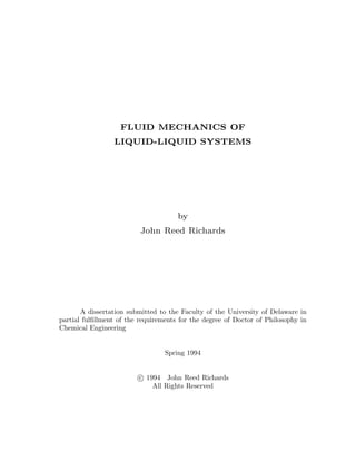
Consider the material pillbox in Figure 2.1 with volume V straddling a
discontinuous moving interface with area A. The domain is decomposed as:
V = ¯V ∪ A (2.1)
where the overbar denotes a bulk-phase quantity and the locus of the entire volume
of the pillbox V is the union of the locus of points of the bulk volume ¯V and the
locus of points of the interface A. The bulk volume ¯V is the union of the bulk
volumes ¯V1 and ¯V2 on either side of the interface:
¯V = ¯V1 ∪ ¯V2 (2.2)
The total closed surface ∂V bounding the volume V can be decomposed as the
union of the surface area bounding the bulk volume ∂ ¯V and the closed curve
bounding the interface ∂A:
∂V = ∂ ¯V ∪ ∂A (2.3)
45. 19
with the area enclosing the bulk volume ∂ ¯V the union of the areas A1 and A2
enclosing the bulk volumes on either side of the interface:
∂ ¯V = A1 ∪ A2 (2.4)
Here the interfacial normal, n, is defined as pointing from phase 2 to phase 1.
2.1.1 Linear Momentum Balance
We can write a balance for linear momentum for the pillbox:
d
dt
¯V
ρv dV +
A
ρs
vs
dA
=
∂ ¯V
P · dS +
∂A
Ps
· dL+
¯V
ρg dV +
A
ρs
g dA
(2.5)
The first term on the left hand side of this equation represents the rate of change
in the total amount of linear momentum ρv per unit volume of V . The second
term on the left represents the rate of change in total amount of linear momentum
ρsvs per unit area in the interfacial region A. The first term on the right is the
diffusive flux of linear momentum into V through ∂ ¯V , where P is the (tensile)1
stress tensor in units of force per unit area of ∂ ¯V , and dS is the outward directed
normal to ∂ ¯V . The second term on the right hand side of equation (2.5) is the
diffusive flux of linear momentum into A through ∂A, where Ps is the (tensile)
surface stress tensor in units of force per unit length of ∂A, and dL is the outward
directed normal to ∂A. The third term is the rate of supply of momentum to V by
the action of long range forces (in this case gravity), where ρg is the gravitational
force per unit volume of V . The fourth term is the rate of supply of momentum
to A by the action of long range forces, where ρsg is the gravitational force
per unit area of ∂A. At this point we need to use four theorems which are
presented here without proof (Edwards et al., 1991). Before doing so, we define
the following operators and tensors. Let the position vector x = x1, x2, x3 be the
1
Some texts (Bird et al., 1960) define P as compressive with the appropriate sign change.
46. 20
Fluid 1
F = 0
A
Interface
n^ A1
A2
Fluid 2
F = 1
n^
V2
V1
dS1
dL
dS1
dS2
dS2
∂A
n
n
Figure 2.1: A material volume V which intersects the discontinuous interface
between fluids 1 and 2.
3-D Cartesian coordinates of a point in space, let q1, q2, q3 be the coordinates
in another general curvilinear coordinate system and let the functional relation
between the two coordinate systems be x = x q1, q2, q3 . Let q1, q2 be the 2-D
surface coordinate system and let the equation of the surface be xs = xs q1, q2
47. 21
(Edwards et al., 1991). We can construct basis vectors for these 3-D and 2-D
spaces:
gi ≡
∂x
∂qi
, (i = 1, 2, 3); aα ≡
∂xs
∂qα
, (α = 1, 2) (2.6)
The spatial and surface reciprocal basis vectors can be defined such that:
gi·gj
≡ δj
i , (i, j = 1, 2, 3); aα·aβ
≡ δβ
α, (α, β = 1, 2) (2.7)
Where δj
i is the Kronecker delta:
δj
i ≡
1, if i = j
0, if i = j
(2.8)
The spatial and surface gradient operators are then defined as:
≡
3
i=1
gi ∂
∂qi
; s ≡
2
α=1
aα ∂
∂qα
(2.9)
We can further define the dyadic spatial and surface unit tensors:
I ≡
3
i=1
gi
gi; Is ≡
2
α=1
aα
aα = I − nn (2.10)
The surface unit normal is constructed using the surface basis vectors:
n ≡
a1×a2
|a1×a2|
(2.11)
The gradient along a direction normal to the interface is defined as (Brackbill et
al., 1992):
N ≡ n (n· ) (2.12)
and its gradient tangent to the interface is the surface gradient operator:
s = − N (2.13)
48. 22
Theorem 2.1 The surface divergence theorem for a surface A surrounded by a
closed curve ∂A:
∂A
Ps
·dL =
A
s· (Is·Ps
) dA (2.14)
Theorem 2.2 The surface divergence theorem for a fluid volume V possessing a
surface of discontinuity A:
¯V
·P dV =
∂ ¯V
P · dS −
A
(P1 − P2) ·n dA (2.15)
Theorem 2.3 The volumetric Reynolds transport theorem for a moving volume
¯V (t):
d
dt
¯V
ρv dV
=
¯V
∂
∂t
ρv + · (vvρ) dV (2.16)
Theorem 2.4 The surface Reynolds transport theorem for a convected material
surface A(t):
d
dt
A
ρs
vs
dA
=
A
∂
∂t
ρs
vs
+ s· (vs
vs
ρs
) dA (2.17)
Using these four theorems the momentum balance becomes:
¯V
∂
∂t
ρv + · (vvρ) dV +
A
∂
∂t
ρs
vs
+ s· (vs
vs
ρs
) dA
=
¯V
·P dV +
A
(P1 − P2) ·n dA +
A
s· (Is·Ps
) dA
+
¯V
ρg dV +
A
ρs
g dA
(2.18)
49. 23
or:
¯V
∂
∂t
ρv + · (vvρ) − ·P−ρg dV
+
A
∂
∂t
ρs
vs
+ s· (vs
vs
ρs
) − s· (Is·Ps
) − ρs
g − (P1 − P2) ·n dA = 0
(2.19)
Since V and A are arbitrarily chosen this yields the bulk and surface linear
momentum equations:
∂
∂t
ρv + · (vvρ) − ·P − ρg = 0 (2.20)
∂
∂t
ρs
vs
+ s· (vs
vs
ρs
) − s· (Is·Ps
) − ρs
g − (P1 − P2) ·n = 0 (2.21)
Also, for the entire domain of V = ¯V ∪ A including the interfacial region we have:
¯V
∂
∂t
ρv + · (vvρ) − ·P − ρg dV
+
¯V
∂
∂t
ρs
vs
+ · (vs
vs
ρs
) − s· (Is·Ps
) − ρs
g δ{n· (x − xs)} dV
+
¯V
[− (P1 − P2) ·n ] δ{n· (x − xs)} dV = 0
(2.22)
where δ{n· (x − xs)} is the Dirac delta function for the scalar normal distance
from the interface, n· (x − xs) defined such that
∞
−∞ f (x) δ (x − a) dx = f (a).
Collecting terms, equation (2.22) becomes:
¯V
∂
∂t
ρv + · (vvρ) − ·P−ρg − [(P1 − P2) ·n] δ{n· (x − xs)} dV = 0 (2.23)
Since the volume V is arbitrary we have what we call the volumetric linear
50. 24
momentum equation:
∂
∂t
ρv + · (vvρ) = ·P + ρg + (P1 − P2) · n δ{n· (x − xs)} (2.24)
2.1.2 Mass Balances
Equations (2.20) and (2.21) are in fact quite general in that if we substitute
mass density for momentum density (ρ → ρv, ρs → ρsvs) into the bulk and surface
momentum equations (2.20) and (2.21), and assume that the diffusive flux of mass
term is zero (P, Ps), and the rate of supply of mass term is zero (ρg, ρsg → 0),
we obtain the bulk and surface continuity equations:
∂ρ
∂t
+ · (vρ) = 0 (2.25)
∂ρs
∂t
+ s· (vs
ρs
) = 0 (2.26)
Using the continuity equations, (2.25) and (2.26), the bulk, surface and volumetric
momentum equations then become (using the fact that evidently Is·Ps = Ps,
Edwards et al., 1991):
ρ
∂v
∂t
+ (v· ) v = ·P+ρg (2.27)
ρs ∂vs
∂t
+ (vs
· s) vs
= s·Ps
+ ρs
g+ (P1 − P2) ·n (2.28)
ρ
∂v
∂t
+ (v· ) v = ·P + ρg + (P1 − P2) ·n δ{n· (x − xs)} (2.29)
If we invoke the condition that ρ =constant (incompressible fluids) in both phases
the bulk continuity equation becomes:
·v = 0 (2.30)
However, it is noted by Edwards et al. (1991) that since ρs is not generally constant
in the interfacial region:
s·vs
= 0 (2.31)
51. 25
2.1.3 Constitutive Equations
Let us start with the constitutive equation for the bulk stress tensor of a
Newtonian fluid:
P = −pI + τ (2.32)
τ = κ −
2
3
µ (I:D) I + 2µD (2.33)
D =
1
2
( v) + ( v)†
(2.34)
where p is the pressure, τ is the viscous stress tensor, κ is the dilatational viscosity,
µ is the shear viscosity, D is the rate of deformation tensor, and the double dot
product follows the nesting convention mn:pq = (n·p) (m·q). If we invoke the
condition that ρ =constant (incompressible fluids) in both bulk phases, equations
(2.32)–(2.34) become (since I:D = ·v = 0):
τ = 2µD (2.35)
By analogy the (Boussinesq-Scriven) constitutive equation for the surface
stress tensor is (Scriven, 1960):
Ps
= σIs + τs
(2.36)
τs
= (κs
− µs
) (Is:Ds) Is + 2µs
Ds (2.37)
Ds =
1
2
( svs
) ·Is + Is· ( sv)†
(2.38)
where σ is the interfacial tension, τs is the surface viscous stress tensor, κs is the
surface dilatational viscosity, µs is the surface shear viscosity, and Ds is the surface
rate of deformation tensor. Assuming that the surface is clean κs ≈ µs ≈ 0, then
equations (2.36) to (2.38) become simply:
Ps
= σIs (2.39)
52. 26
2.1.4 Surface Stress Boundary Condition
Now, if it is assumed that there is no material accumulation at the interface
so that ρs ≈ 0, our surface linear momentum equation (2.28) becomes:
− (P1 − P2) ·n = s·Ps
(2.40)
If we insert the constitutive equation (2.39) into (2.40) we obtain the surface stress
boundary condition:
− (P1 − P2) ·n = s· (Isσ) = ( s·Is) σ + Is· ( sσ) = 2Hσn + sσ (2.41)
where the mean curvature H is defined by:
2H ≡ − s·n (2.42)
Here we have used the relation [ s·Is] = 2Hn (Edwards et al., 1991). Note that
from this definition, (2.42), H is a positive scalar when the unit surface normal n
points in the direction of the concave side of the surface.
2.2 Interfacial Relations
2.2.1 CSF Method Formulation
Equations for mass (2.25), momentum (2.30), constitutive equations (2.32)
to (2.34) and equation (2.41) as the boundary condition at the free surface can be
used to solve multiphase flow problems (e.g., the derivation of the Young-Laplace
equation in appendix B). However, an alternative route, more convenient for finite
volume numerical methods, is to use the surface momentum equation (2.29). This
includes the surface forces as accelerations and constitutes the Continuous Surface
Force Method (CSF) of Brackbill et al. (1992).
If we insert the surface stress boundary equation (2.41) into the volumetric
53. 27
momentum balance (2.29) we obtain:
ρ
∂v
∂t
+ (v· ) v = ·P + ρg − (2Hσn + sσ) δ{n· (x − xs)} (2.43)
At this point, we need a mathematical description of the interface. The derivation
of the following equations given here (Richards et al., 1993) follows a slightly
different path from that in the CSF reference (Brackbill et al., 1992), but reaches
the same final result. The equation of the interface can be expressed by the
(discontinuous) Volume of Fluid (VOF) function:
F(x) ≡
0, fluid 1
1/2, at the interface
1, fluid 2
(2.44)
We may also define a “mollified” VOF function, ˜F(x), such that within a transition
region of finite thickness, h, it is a smoothly varying series of nested contours where
0 ≤ ˜F ≤ 1. A definition for such a function is (Brackbill et al., 1992):
˜F(x) ≡
1
h3
V
F(xs) (xs − x) d3
xs (2.45)
lim
h→0
˜F(x) = F(x) (2.46)
where (xs − x) is an interpolation function (such as a B-spline) with the following
properties (in addition to being differentiable and decreasing monotonically with
increasing |x|):
V
(x) dV = h3
(2.47)
(x) = 0 for |x| ≥
h
2
(2.48)
The CSF interface normal (which points from fluid 1 into fluid 2) is defined
by:
ˆn ≡
F
| F|
(2.49)
54. 28
Thus, the CSF choice of normal is the opposite of the Edwards et al. (1991)
normal: ˆn = −n. The surface boundary condition becomes with the CSF normal
definition:
(P1 − P2) ·ˆn = κσˆn + sσ (2.50)
and the surface momentum equation (2.43) now becomes:
ρ
∂v
∂t
+ (v· ) v = ·P + ρg + (κσˆn + sσ) δ{ˆn· (x − xs)} (2.51)
where the mean curvature, κ (not to be confused with dilatational viscosity), is
now:
κ ≡ − s·ˆn = − 2H (2.52)
Note that κ is a positive scalar when the unit surface normal ˆn points in the
direction of the concave side of the surface. Equations (2.50)–(2.52) indicate that
the pressure is greater on the concave side of the interface, and that if there is a
surface tension gradient, the fluid will flow from regions of lower to higher surface
tension (Landau and Lifshitz, 1959). For example, the effect of a non-zero surface
tension gradient (known as the Marangoni effect) due to a non-zero temperature
gradient has been recently investigated by Sasmal and Hochstein (1993) in the
context of the VOF method.
The expression for curvature can be simplified (Brackbill et al., 1992):
κ ≡ − ( s·ˆn)
= − [Is· ] ·ˆn
= − [{I − ˆnˆn} · ] ·ˆn
= − [ − ˆnˆn· ] ·ˆn
= − ( ·ˆn) + [ˆnˆn· ] ·ˆn
(2.53)
55. 29
The last term in equation (2.53) is:
[ˆnˆn· ] ·ˆn = ˆn· [(ˆn· ) ˆn] = ˆn· [ˆn· ˆn] = ˆn·
1
2
(ˆn·ˆn) − ˆn× [ ׈n] (2.54)
Now (ˆn·ˆn) = 0 and the last term in equation (2.54) becomes (Aris, 1989):
[ ׈n] = [ × F] = 0 (2.55)
so that finally we can replace s·ˆn with ·ˆn in equation (2.51):
κ = − ( ·ˆn) (2.56)
We can define the volumetric surface force from the right hand side of the volu-
metric momentum equation (2.51) neglecting the surface tension gradient term,
Fsv(x), for an interface of finite thickness as:
lim
h→0
Fsv(x) ≡ σ κ(x) ˆn(x) δ{ˆn(xs)· (x − xs)} (2.57)
Now the VOF equation of the interface can be written (Richards et al., 1993):
F(x,t) = (F2 − F1) H {ˆn(xs)· (x − xs)} (2.58)
where H(x) is the Heaviside step function:
H(x) ≡
1, for x ≥ 0
0, for x < 0
(2.59)
We can take the spatial gradient of equation (2.58), and by using the chain rule
obtain:
F(x) = (F2 − F1) H{ˆn(xs)· (x − xs)}
= (F2 − F1) ˆn(x) δ{ˆn(xs)· (x − xs)}
= lim
h→0
˜F(x)
(2.60)
56. 30
Inserting equation (2.60) into the volumetric surface force definition (2.57):
Fsv(x) = σ κ(x)
˜F(x)
F2 − F1
(2.61)
so that finally (with F2 − F1 ≡ 1):
lim
h→0
Fsv(x) = σ κ(x) F(x) (2.62)
If we restrict ourselves to situations where the surface tension gradient sσ = 0,
the surface momentum equation (2.51) becomes:
ρ
∂v
∂t
+ (v· ) v = ·P + ρg + σ κ(x) F(x) (2.63)
2.2.2 Interface Kinematic Relation
Suppose we have a point fluid particle moving through 3-D space. At time
t = 0 the position of the particle is specified by ξ and at a later time the particle
is at position x. The spatial position can be represented parametrically by (Aris,
1989):
x = x (ξ, t) (2.64)
The point trajectory equation may be inverted (assuming a non-singular Jacobian,
i.e., that the fluid particle does not break up during the motion or that two particles
do not occupy the same space at the same time) to give the initial position or
material coordinates of the particle which is at any position x at time t:
ξ = ξ (x, t) (2.65)
Any property of the fluid, say (ξ, t), may be observed along the particle path.
The description of the change of this property (ξ, t) may be changed into a
spatial description by equation (2.65):
(x, t) = [ξ (x, t) , t] (2.66)
57. 31
This says that the value of the property at position x and time t is the same as
the value appropriate to the particle at (x, t). The material description may be
derived from the spatial description (2.64):
(ξ, t) = [x (ξ, t) , t] (2.67)
meaning that the value as seen by the particle at time t is the value of the position
it occupies at that time. Let the change in the property observed at a fixed point
x be:
∂
∂t
≡
∂
∂t x
(2.68)
Let the change in the property observed when moving with the particle be:
D
Dt
≡
∂
∂t
(2.69)
The velocity of the particle is the material derivative of its position ( = xi) and
is defined by:
v (x, t) ≡
∂x
∂t
(2.70)
The two derivatives (2.68), (2.69) may be related by differentiating the material
description (2.67) and using the chain rule:
D
Dt
≡
∂
∂t
=
∂
∂t
(ξ, t) =
∂
∂t
[x (ξ, t) , t] =
∂
∂t x
+
∂x
∂t
·
∂
∂x t
(2.71)
or:
D
Dt
=
∂
∂t
+ v · (2.72)
Let the interface consist of the same material particles moving at velocity vs = vs
1
= vs
2 and let the material function describing their position be the VOF function
( =F(x, t)) as defined above. Then using the VOF definition (2.44) the kinematic
equation for the interface becomes by differentiation:
DF
Dt
=
∂F
∂t
+ vs
· F = 0 (2.73)
58. 32
This equation assumes that the particles move at the same velocity as the interface,
which may not be the case if mass transfer is occurring between the interface and
the bulk phases (Edwards et al., 1991).
59. Chapter 3
NUMERICAL IMPLEMENTATION OF THE
VOLUME OF FLUID–CONTINUOUS
SURFACE FORCE METHOD
The purpose of computing is insight, not numbers. This motto is
often thought to mean that the numbers from a computing machine
should be read and used, but there is much more to the motto. The
choice of the particular formula, or algorithm, influences not only the
computing but also how we are to understand the results when they
are obtained . . .Thus computing is, or at least should be, intimately
bound up with both the source of the problem and the use that is going
to be made of the answers – it is not a step to be taken in isolation
from reality.
R. W. Hamming (1986)
The solutions to complex free surface flow problems involve the solution
of the equations of motion and continuity for the two fluids subject to specified
boundary conditions and their numerical solution is briefly reviewed in section 1.3.
In this dissertation we use the Eulerian Volume of Fluid (VOF) method (Hirt
and Nichols, 1981), in which a marker function convected by the flow is used to
track the interface. The major incentive for using the VOF method is that it
allows for the description of highly complex interfaces such as those encountered
in multiphase flows. Reasonable accuracy is attainable with elemental control
volume balances, yet the method is relatively simple to implement. This algorithm
is publicly available in a two-fluid, 2-D program called SOLA-VOF (Nichols et al.,
1980). A 3-D version called FLOW-3D (Hirt, 1988) is also available commercially.
More recently a one-fluid program, RIPPLE, which implements the Continuum
33
60. 34
Surface Force (CSF) algorithm and incorporates various improvements in the one-
fluid VOF algorithm, has been introduced by Kothe et al. (Kothe et al., 1991;
Brackbill et al., 1992). In this chapter we describe how we have combined the two-
fluid capability of the SOLA-VOF algorithm with the free surface implementation
of the CSF algorithm to investigate problems that involve transient 2-D free surface
flows with two immiscible fluids.
The source code for SOLA-VOF has been extensively modified and the
resulting code tested for consistency and accuracy with numerous test problems. It
has been rewritten to accommodate the addition of the second fluid with arbitrary
viscosity, to correct the incorporation of the viscous stress terms, and to add a
superior surface tension algorithm. The original SOLA-VOF 2-D program (Nichols
et al., 1980) is well suited for high Reynolds number flows, including those involving
free surfaces. Among the latter, however, it is better suited for gas-liquid than
for liquid-liquid systems, and relaxing this limitation has been an important part
of our efforts. Thus, we have implemented extensive modifications in the original
program. Both planar and axisymmetric 2-D flows can be simulated.
This chapter outlines the numerical methods used in combining the VOF
(Hirt and Nichols, 1981) and CSF (Brackbill et al., 1992) algorithms. Although
the VOF references describe the algorithm for the iteration procedure, very little
justification is provided there. This chapter addresses this issue.
3.1 Governing Equations in a Cylindrical Coordinate System
It is assumed that the flow in each phase is axisymmetric, viscous, and
incompressible. The continuity equation (2.30) given in cylindrical, axisymmetric
coordinates (r, z) as:
∂u
∂r
+
∂v
∂z
+
u
r
= 0 (3.1)
61. 35
where (u, v) are the radial, axial components of the velocity field respectively. The
dynamic momentum equation (2.63) becomes:
ρ
∂u
∂t
+ u
∂u
∂r
+ v
∂u
∂z
= −
∂p
∂r
+
∂τrr
∂r
+
∂τzr
∂z
+
τrr
r
+ ρgr + σκ
∂F
∂r
(3.2)
ρ
∂v
∂t
+ u
∂v
∂r
+ v
∂v
∂z
= −
∂p
∂z
+
∂τrz
∂r
+
∂τzz
∂z
+
τrz
r
+ ρgz + σκ
∂F
∂z
(3.3)
where p is the pressure, gr, gz are the radial and axial components of the gravita-
tional acceleration, τrr, τzr, τrz, τzz are the components of the Newtonian stress
tensor from equations (2.32) and (2.35):
τrr = 2µ
∂u
∂r
, τzr = τrz = µ
∂v
∂r
+
∂u
∂z
, τzz = 2µ
∂v
∂z
(3.4)
and κ is the curvature of the liquid-liquid interface (Kothe et al., 1991; Brackbill
et al., 1992) from equation (2.56),
κ = − ( ·ˆn) (3.5)
where the unit normal (directed into fluid 2),
ˆn =
˜n
|˜n|
(3.6)
is derived from a normal vector,
˜n = F (3.7)
The evolution equation (2.73) for the fluid function marker field, F, is:
∂F
∂t
+ u
∂F
∂r
+ v
∂F
∂z
= 0 (3.8)
The density and viscosity fields are obtained from:
ρ = ρ1 (1 − F) + ρ2F (3.9)
62. 36
µ = µ1 (1 − F) + µ2F (3.10)
Note that the interfacial surface forces are incorporated as body forces per
unit volume in the momentum equations (3.2) and (3.3) rather than as boundary
conditions. Instead of a surface tensile force boundary condition applied at a
discontinuous interface of the two fluids, a volume force is used which acts on fluid
elements lying within a transition region of finite thickness. The CSF formulation
makes use of the approach taken in numerical simulations that discontinuities
can be approximated, without increasing the overall error of approximation, as
continuous transitions within which the fluid properties vary smoothly from one
fluid to the other over a distance of O(h), where h is a length comparable to
the resolution of the computational mesh. Surface tension, therefore, is felt
everywhere within the transition region through the volume force included in the
momentum equations. A derivation is given in appendix A which shows that the
CSF formulation is equivalent in the limit of infinitesimal interfacial thickness h to
the classical description of these forces as boundary conditions at a discontinuous
interface, and supplements the previous derivation in the CSF references (Kothe
et al., 1991; Brackbill et al., 1992). It can be seen that this formulation is similar
to the approach taken in the finite element method in that the free surface forces
are included in the momentum integral residual equation (Georgiou et al., 1988;
Cuvelier and Schulkes, 1990; Malamataris and Papanastasiou, 1991). Also note
that interfacial surface tension is presumed constant, and surface tension gradient
induced stresses are not included in equations (3.2) and (3.3). Effects such as
surface tension gradient and surface dilatational and shear viscosities can, in
principle, be included, (Scriven, 1960) and may be important if surface active
agents are present.
Massless marker particles can be placed in the flow to follow fluid elements
if necessary for comparison with experimental results. Local velocities (up, vp)
of the marker particles are used to update the positions by use of the kinematic
63. 37
relations:
dr
dt
= up,
dz
dt
= vp (3.11)
For 2-D axisymmetric flows the streamfunction ψ can be defined, as usual,
in order for the velocity to be divergence free (i.e., by satisfying the incompress-
ibility condition):
u =
1
r
∂ψ
∂z
, v = −
1
r
∂ψ
∂r
(3.12)
Then the streamfunction ψ can be calculated from the following Poisson equation
(obtained by differentiating equations (3.12)), given the velocity field:
∂2ψ
∂r2
+
∂2ψ
∂z2
= r
∂u
∂z
−
∂v
∂r
− v (3.13)
These equations are to be solved subject to appropriate boundary conditions
discussed in section 3.6 (see, for example, chapter 5).
3.2 Momentum and Continuity Finite Differencing
The momentum equations are finite-differenced on a locally variable, stag-
gered mesh using the control volume approach, as illustrated in Figure 3.1. As
Figure 3.1 shows, the radial velocity ui+1
2 ,j and axial velocity vi,j+1
2
are centered
at the right face and top face of each cell respectively, whereas the pressure, pi,j,
and marker function, Fi,j, are located at the center. The details can be found in
Nichols et al. (1980) and Hirt and Nichols (1981), while an introduction to control
volume approaches on staggered meshes can be found in Patankar (1980).
The equations (3.1) to (3.4) are solved for the variables u, v, and p at each
time step by an iterative method, a form of successive overrelaxation (SOR) that
will now be described. We may rewrite the equations explicitly in velocity and
implicitly in pressure for the (i, j)th cell with an Euler scheme from the current
time n to the new time n + 1, accurate to first-order in time:
∂u
∂r
+
∂v
∂z
+
u
r
n+1
= 0 (3.14)