SlideShare a Scribd company logo
1 of 33
Download to read offline
1
Weather and Climate Error in a Nested
Regional Climate Model: OLR and
Precipitation
NWP Final Project: Fall 2012
Authors: James S. Brownlee, Angie R. Lassman, Robert S. James
Date Submitted: December 07, 2012
Abstract
Global Climate Models (GCMs) are used heavily to conduct research on how the atmosphere
will progress into the future. However, the errors within these models can quickly become large
due to the amount of complicated processes that occur in the atmosphere on a variety of time
scales. An important aspect of this is how quickly does a GCM’s error become indistinguishable
from the mean climate error. Once this occurs, it is difficult to get accurate weather forecasts
from these models. In order to reduce errors in these models, it is important to analyze many
different output quantities from them. For our research, we analyzed a nested regional climate
model temporally, ranging from daily to seasonally to yearly, and spatially, focusing on the
errors over land and ocean. Our goal for this research is to be able to explain why errors in this
model are occurring and what could be done to correct them.
2
1) Introduction
All atmospheric models are created and run knowing that they will inherently contain
some error in their output, no matter how good the equations or physical parameterizations are,
which increases as the model generates a forecast field becomes farther from its initial state
(Allen et al. 2006). Being able to analyze and understand these errors is a method for
continuously improving atmospheric models. One way in which to know how far a model’s
forecast field has strayed from the truth is to compare it to observations at the time in which the
forecast is valid for, which is the emphasis of our research for this paper.
In this study, we will be analyzing output from a nested regional climate model (NRCM),
focusing on precipitation (both convective and non-convective components) and how it relates to
observed outgoing longwave radiation (OLR). In addition, we will provide some insight of the
various errors found in this model, including how quickly precipitation errors within the model
equal and surpass the mean climate error. The model output is from a version of the Weather
Research and Forecasting model (WRF), which has a horizontal resolution of 36 km, a zonal
domain of 0°W to 360°W, a meridional domain of 30°S to 45°N, and a daily time interval. Our
study will only focus on this domain, which is the coarsest of three within the NRCM. Also, our
research will concentrate on the meridional domain of 30°S to 30°N, and keeping the zonal
domain intact (Fig. 1), to be able to more easily complete an analysis between the northern and
southern hemispheres. The time domain for this simulation was defined between 1 January 1996
and 31 December 2000. Our investigation has been aided by computer software from the Center
for Ocean-Land-Atmosphere Studies called the Grid Analysis and Display System (GrADS),
which allowed us to display the model data.
3
First, we will look at a simple error analysis of the modeled output compared with
observation data. This will be done using three time delineations: seasonally, annually, and
overall mean error. The second portion of our research will be a statistical analysis of the model
errors, as well as the seasonal and mean trends in OLR data. Finally, we will discuss the
differences in the convective and non-convective components of the model output, and complete
an analysis of zonal and meridional averages in the model output. Combined, these research
points will help us to understand errors in atmospheric models; such as the one we are examining,
and why they may be occurring.
2) Error Analysis
2.1) Seasonal Error
The first figure created is an error analysis of the WRF model output precipitations and
the observed precipitation data. The model output uses the sum of the convective and non-
convective precipitation while the observed data is the total rain. The time delineation is
seasonal from 1996 to 2000, divided into sections from March to May, June to August,
September to November, and December to February at 30°N to 30°S. The red and blue shading
scale values in Fig. 2 are determined by subtracting the observed precipitation from the model
precipitation. Therefore, the positive values correlate to model overestimation while negative
values are model underestimation.
The pattern of seasonal variances between the Northern and Southern Hemispheres in Fig.
2 leads to the theory that the incoming radiation is indirectly affecting the over or
underestimation of precipitation in the WRF model (Thornton and Running 1999; Richardson
1981). It is obvious in Figs. 2A, D that from December to May the southern hemisphere is
receiving the most incoming solar radiation. This is also the case when focusing on Figs. 2B, C
4
except during this time period, the Northern Hemisphere is receiving more incoming solar
radiation. During those time frames, these locations experience a large overestimation in total
precipitation by the NRCM. The fact that convection occurs when the Earth’s surface within a
conditionally unstable or moist atmosphere is warmer than its surroundings which leads to
evaporation and rising motion in the air column. This process promotes the formation of a
convective cloud, such as cumulonimbus or cumulus congestus. The solar radiation ties in with
this process during the diurnal heating of the earth's surface, with more incoming solar radiation
usually correlating to larger amounts of convective precipitation (Winslow and Hunt Jr. 2001).
Also, precipitation is known to be very high near the equator due partially to the influence of the
Intertropical Convergence Zone (ITCZ) (Waliser and Gautier 1993). This is due to the
convergence of the northeast trade winds and southeast trade winds in a low-pressure zone
coupled with the high ability of convection, which then promotes lifting in the air column. The
ITCZ is clearly defined with the NRCM overestimating precipitation on each of the seasonal
subfigures in Fig. 2. Because this region is usually known for its high amount of precipitation, it
is likely that the model has a bias in the dynamic parameters of this region, thus causing the
overestimation (Waliser and Gautier 1993). However, the location of this high precipitation
region or ITCZ does however vary throughout the year. The northward and southward seasonal
movement of this zone can be seen when comparing each subfigure in Fig. 2. One issue that
becomes apparent when analyzing this figure is the failure to depict the seasonal transition of the
ITCZ. The secondary meridional circulation induced by convective momentum transport (CMT)
within the ascending branch of the Hadley circulation is a missing dynamical mechanism that
can cause common failure of general circulation models (GCMs) in simulating seasonal
migration of ITCZ precipitation maximum across the equator (Janowiak et al. 1995; Wu 2003).
5
This failure is created from the model bias precipitation peak remaining north of the equator
during November through March.
2.2) Annual Error
Another way to analyze climate and weather errors in models is to examine them from an
annual point of view. Fig. 3 is organized as yearly data from 1996 to 2000. The annual data
shown in this figure is very similar to above explanation of Fig. 2, as it is the error of the model
output (sum of convective and non-convective precipitation) compared with total rain
observations. The purpose of comparing the data by year is to determine if specific
meteorological or oceanographic climatological events occurring in that time period have
affected the models output. With this said, an occurrence would have to be very large for its
impact to show up on an entire years model data. Therefore, eliminating all mesoscale events
that may have occurred during the time period. After some research, it was discovered that one
of the strongest El Niño event ever was recorded in 1997 to 1998 (Chambers et al. 1999;
Williamson et al. 2000). An El Niño is an anomalous ocean warming, occurring about every five
years, which generates a dominant source of climate variability across the globe. The
atmospheric component linked to El Niño is the Southern Oscillation based upon research from
many studies (Rasmusson and Carpenter 1983; McPhaden et al. 1998). This is a fluctuation of
surface air pressure at sea level in the tropical eastern and western Pacific Ocean. Experts believe
that these atmospheric and oceanic temperature anomalies collaborate together forming the
phenomena called El Niño Southern Oscillation (ENSO) (Trenberth 1997). ENSO is likely
related to many unusual climatic events occurring around the globe, such as increase in monsoon
rainfall, drought and an extraordinary number of storms (Rasmusson and Wallace 1983). When
comparing the effects of ENSO to the annual model and observed data characteristic of ENSO
6
are apparent in Fig. 2B during the year of 1997. Studies of this event show that heavy monsoons
occurred as an affect of ENSO. While the Southern Oscillation isn’t the only factor influencing
the monsoon seasons in Southeast Asia, there is a close association between ENSO and the
summer monsoon rainfall, based on how precipitation was distributed (Ropelewski and Halpert
1996). Fig. 3B, compared to the rest of the subfigures, shows a high amount of overestimation in
the usually wet region of Southeast Asia. This leads to the idea that the model is positively
biased towards heavier precipitation. Also, the interannual change in the extratropical
wintertime jet stream over the western and central Pacific is highly influenced by ENSO due to
the close relation to the distribution of tropical convection across Indonesia and the tropical
Pacific. The Pacific Ocean Basin and the Indian subcontinent have both shown precipitation
patterns directly related to the ENSO (Ropelewski and Halpert 1987). These variations change
the location of the jet stream, extending it further over the eastern Pacific and towards the
equator. These atmospheric conditions then play a role in enhancing storminess and above-
normal precipitation at lower latitudes of both North and South America. This is apparent again
in Fig. 3B off the coast of South America. Annually organizing the data in Fig. 3 clearly defines
the heavier precipitation regions along the ITCZ by the NRCM overestimation of precipitation.
2.3) Mean Climate Error
The mean climate error of the modeling using the sum of the convective and non-
convective precipitation compared with the total rain observed is shown in Fig. 4. This
comparison is helpful when looking for an overall prominent climatologically error in the model.
For this figure, we used the five-year averages of model estimated and observed precipitation
over the entire time domain of the model from 1 January 1996 to 31 December 2000. The model
overestimation is again shaded in the darker red and model underestimation is shaded blue. This
7
image reinforces the idea that the WRF model overly pronounces the relatively wetter regions
along the tropical belt, such as the ITCZ and areas associated with monsoons or large amount of
rain. This also carries over into the dry regions with higher values of underestimation such as
areas of Australia and the desert regions of Africa. This regional model continually shows an
overestimation over water regions, such as the Indian Ocean, Western Pacific, and Eastern
Pacific and along the ITCZ.
3) Statistical Analysis
3.1) Root Mean Squared Error
Statistically analyzing data for errors can be helpful when looking for specific deviations
in data or certain patterns (Wilks 1995, section 7.5.2). For the purposes of our research, we used
the Root Mean Squared Error (RMSE) of the model output (sum of convective and non-
convective precipitation) compared with the observations (total rain). The RMSE is defined for
our purposes as Equation 1, where ym is the model data at time-step “m”, om is the observation
data at time-step “m” and “M” is the total number of time-steps in the data. A perfect forecast
will yield an RMSE value of zero, but the limit of RMSE values is infinite as errors become
larger.
                                                                                                                    𝑅𝑀𝑆𝐸 =
(𝑦! − 𝑜!)!!
!!!
𝑀
                                                                                                                                      (1)
The RMSE values shown in Fig. 5 were taken at each individual grid point, over the
entire five-year simulation. The results in this figure correlate well with the discussion of Figs. 2,
3, and 4 as the areas of high over or under estimation correlate to areas of high RMSE. The
highest RMSE values are mainly focused in the Indian Ocean, Western Pacific Ocean, and just
of the coast of northwestern South America.
8
3.2) Error Growth
Fig. 6 depicts the error growth of precipitation in the model domain. A calculation of
precipitation RMSE for each individual day for the month of January 1996 and the average
climate precipitation root mean squared error over the entire 5-year simulation is shown in Fig. 6.
The purpose of this image is to analyze how soon after model initialization does the precipitation
errors match up to the mean climate error. Using this method, our results show that our NRCM
took approximately seven days the for precipitations errors to catch up to the mean climate error,
calculated over the entire five-year period, and seemed to oscillate around that mean for the
remainder of the month of January. The usage of the model for forecast purposes on any given
day after 8 January 1996 would have yielded very inaccurate results, and thus the error seen in
the climatological mean would be just as good, if not better, than the forecast output from this
NRCM. In order to receive accurate precipitation forecasts and creating forecasts, it would be
necessary to run the model at least every 7 days in order to achieve lower forecast errors than the
climatological average. Since the only available initialization time for our study was 1 January
1996, we are unable to see if this is a continuous error in this model if it was able to be initialized
more often, or if there was another underlying issue causing the RMSE to rise so quickly. To
determine this we would need to be able to initialize this model and numerous times to see if the
error is reoccurring. During this process it would also be necessary to see how it changes based
on the time of initialization, instead of only having output on a daily time scale.
4) Comparison of Precipitation Error to Outgoing Longwave Radiation
4.1) Background on Outgoing Longwave Radiation Techniques
9
In this section of the paper, an analysis of the relationship between outgoing longwave
radiation (OLR), cloud cover, and precipitation intensity will be carried out over the domain that
is described in the introduction section. However before getting into the analysis of these results,
some background on this subject area is needed. Since 1974, NOAA’s polar orbiting satellites
have been making estimates of OLR (Hartmann and Recker 1986; Xie and Arkin 1998). This
continual input of OLR data has been used in many different meteorological studies. One very
large and prominent area of research in this field has focused on OLR trends over the tropics.
Since there is little variation in temperature over the tropics, any significant changes in OLR are
generally caused by changes in cloud cover. Since the early 1980s, OLR has been used to
quantitatively estimate precipitation, and many studies have made use this technique; this
technique has proven to be a very accurate way to remotely estimate precipitation (Xie and Arkin
1998; Liebmann 1998). Some examples of how this technique is applied in studies will be shown
in the following examples.
Markin and Meisner (1987) used a Geostationary Operational Environmental Satellite
(GOES) Precipitation Index (GPI) to study the correlation between values of OLR and
precipitation over different regions of the tropics. In their study, they found that low values of
OLR correlated with larger amounts of precipitation (Markin and Meisner 1987; Xie and Arkin
1998). In a 1991 study, Janowiak and Arkin developed an equation, using statistical techniques,
which could estimate precipitation based on values of OLR. The techniques used in these studies
considered the total flux of OLR. Deep convective clouds largely control this flux over the
tropics because there is little variation of temperature over such regions of the planet (Xie and
Arkin 1998). Such techniques cannot be used in the same manner over the middle latitudes
because there are larger changes in temperature; these changes in temperature also regulate the
10
OLR flux, and not solely dependent on changes in cloud coverage. In their 1998 study, Xie and
Arkin investigated what the correlations are between global OLR values and precipitation
intensities. In their study, they found a strong relationship between low values of OLR and high
precipitation rates of the tropical regions. Over the middle latitude regions, the cloud coverage-
OLR relationship was not as clearly defined because as stated above, the influence of
temperature changes also controls changes the overall OLR flux.
Trends in OLR can also be used to study the decadal shifts in convection over the tropics.
In their 1997 study, Chu and Wang used statistical methods to study the changes in overall
convection that occurred from 1974-1992. In their study, they found that over the last several
years, OLR values had greatly decreased over the West Central Pacific, over the Indian Ocean,
and over the Bay of Bengal. This was attributed to an overall increase in convective rainfall in
this region, and this increase in rainfall was primarily attributed to a gradual strength in the
monsoon. Over this same period, OLR values increased over Australia, signifying a decrease in
rainfall (Chu and Wang 1997). So, in summary, these studies clearly show that OLR values can
be used to study convective rainfall patterns over the tropical belt. Now that some background on
this subject has been covered, the current analysis of OLR and precipitation over the tropical belt
can be carried out.
4.2) Precipitation Error Correlated to OLR
Fig. 7 shows the overall five-year average of satellite observed OLR values starting on 1
January 1996 and ending on 31 December 2000. Also shown in this figure is the difference
between the five-year average of observed precipitation amounts and the five-year average
model precipitation amounts. The five-year averaged model precipitation is the sum of both
convective and non-convective rainfall. The trend in precipitation in this figure is similar to Figs.
11
2, 3, and 4. The NRCM WRF model overestimated rainfall over regions with large amounts of
precipitation, and it underestimated precipitation in dry regions. So, it could be said that the
model is positively biased towards regions with increased rainfall, and negatively biased towards
regions with little rainfall. These positive and negative biases towards regions of high and low
precipitation have been observed in other model studies, particularly for those where a nested
regional climate model was used (Liu et al. 2012; Murthi et al. 2010). So, in summary, the model
overestimates precipitation in regions with high rainfall and the model underestimates
precipitation in regions with little rainfall.
Despite these biases, the models output clearly does show a strong correlation between
high precipitation regions and outgoing longwave radiation. In Fig. 7, the regions with the
highest precipitation contain the lowest values of OLR. In contrast, the regions with little
precipitation have much higher values of OLR. Over the Indian Ocean, the OLR values are quite
low, and in this region the model output depicts higher precipitation. This also occurs along the
ITCZ, over Central Africa, and over northwestern South America. As shown in Figs. 9 and 10,
the model output shows that convective precipitation dominates in these regions. It is likely that
the model is overestimating the amount of convective precipitation over the tropical regions,
especially over the ocean. A more in depth discussion of this potential error will occur later on
this section of the paper. Over Australia and Northern Africa the OLR values are much higher,
and as shown in the model output, there is little precipitation in these regions. In addition to that,
the model output suggests that there is almost no convective precipitation in these drier regions.
Previous research shows that OLR flux within the tropical belt is mostly controlled by
convective clouds, (Xie and Arkin, 1998; Markin and Meisner, 1987) and this trend is clearly
shown in Fig. 6. The OLR is much lower in regions where there is a local maximum in rainfall
12
and vice versa. So, despite the models bias towards dry and wet regions, the model output when
plotted with satellite derived OLR data, clearly shows the correlation between convective cloud
cover and OLR values. The regions with lower OLR values correlate with higher amounts of
convective rainfall, and the regions with higher OLR have little precipitation and almost no
convective rainfall.
4.3) Seasonal OLR Analysis
Fig. 8 shows the five-year seasonal average of OLR from 1 January 1996 to 31 December
2000. Each of the five-year OLR averages are taken over three month periods, the first being
March, April, and May (Northern hemisphere spring); the second being June, July, and August
(Northern hemisphere summer); the third being September, October, and November (Northern
hemisphere fall); and the fourth being December, January, and February (Northern hemisphere
winter). Similar to Fig. 7, the regions with low OLR values correlate with higher precipitation
rates (Markin and Meisner, 1987). There are several interesting trends that can be deciphered
within these seasonal precipitation patterns. First, during all four seasons, the OLR data clearly
displays the ITCZ over the tropical belt. In addition to that, during the March, April, and May
time period, the heaviest precipitation occurs over the northern part of South America, over
Central Africa, and over the island chains in the central part of the Western Pacific Ocean. By
June, July, and August, the rainfall area decreases over South America, and it increases greatly
over the central part of the Western Pacific and Northern Indian Oceans. Also, the rainfall
increases over the eastern part of the Central Pacific. During the September, October, and
November time period, rainfall remains heavy over the Indian Ocean and over the West Central
Pacific, and it increases over the western part of South America. Secondly, precipitation remains
significant over Central Africa. Over the December, January, and February time period, rainfall
13
increases southward over Central Africa and Central South America; the rainfall belt also shifts
slightly southward over the West Central Pacific moving towards Australia. There are many
global and regional oscillations in the atmosphere and ocean that are responsible for these
seasonal shifts in OLR and rainfall over the tropics. In the next part of this section, some
explanations will show how these seasonal patterns cause the observed seasonal shifts in OLR
and rainfall will be attempted, with the primary focus being on the Central Eastern Pacific,
Central South America, and the Northern Indian Ocean.
The large area of negative OLR values observed over South America during the
December to February time period (Southern hemisphere summer) is primarily driven by the
convergence that occurs along the South Atlantic Convergence Zone (SACZ) and along the
ITCZ (Nogues-Paegle and Mo, 1997; Liebmann et al 1999). This large area of clouds and
precipitation continues through the March to May time period. By the time Southern hemisphere
winter (June to August) comes, the ITCZ has moved northward and the SACZ has weakened,
thus there is noticeable increase in OLR over Central South America due to decreased rainfall
and cloud coverage.
The next area of interest is over the central part of the Eastern Pacific Ocean. Of interest
here is whether or not the large El Nino that occurred at the end of 1997 and at the beginning of
1998 is discernible over the five-year average of seasonal OLR values. From the Northern
hemisphere spring to summer there is a large decrease in OLR values over the central part of the
Eastern Pacific, indicating an increase in sea surface temperatures (SSTs) and deep convection.
From summer to fall, the five-year averaged values of OLR slightly increase, indicating that the
convection has weakened slightly. By winter, the OLR values indicate little to no convection
over this region. In their 2000 study, Wang and Weisberg, analyzed the different changes in
14
atmospheric and oceanic anomalies that occurred during the development and decay of the
1997/1998 El Niño event. In their study, they found that values of OLR began to decrease over
the Central Eastern Pacific between July and September of 1997. During the main stage of the El
Niño, which went from December of 1997 to January of 1998, there was large area of negative
OLR values of the central part of the Eastern Pacific, signifying that widespread deep convection
was occurring over the area during that time. This large area of convection persisted into the
February to April of 1998 time period (Wang and Weisberg, 2000). Comparing this pattern to the
five-year average values of OLR in Fig. 7 suggests that any signal from the 1997/1998 El Niño is
not even noticeable over the five-year seasonal averages. OLR values greatly decreased from
July of 1997 to December of 1997 during the developing El Nino event, while over the five-year
average period, OLR values decrease from summer to winter. Again this suggests that the El
Niño signal is not detectable over the five-year average in observed OLR values. Lastly, it
should be noted that it is possible that the strong convective precipitation estimates in the model
output within Figs. 9 and 10 could have been influenced by the 1997/1998 El Niño event,
however such an assumption is at best inconclusive.
Over the Northern Indian Ocean, the Indian Monsoon controls the seasonal variations in
convection. The monsoon is marked by widespread deep convection over the northern Indian
Ocean during the summer period, especially over the Bay of Bengal (Sengupta and Ravichandran,
2001). In addition to that, convection is enhanced over the eastern part of the Northern Indian
Ocean (Gadgil et al. 2003). This pattern is clearly evident in the 5 year averaged OLR values
over the Bay of Bengal. The lowest OLR values occur during the Northern Hemisphere Summer;
this is when convection is most enhanced over the Bay of Bengal region. Clearly, the five-year
15
averaged OLR values over the Northern Indian Ocean are largely controlled by the seasonal
Indian Ocean monsoon pattern.
5) Convective and Non-convective Precipitation
Figs. 9 and 10 show the five-year average in the areal extent of convective and non-
convective precipitation over the tropical belt from 1 January 1996 to 31 December 2000.
Previous research has shown that when sampling the real atmosphere, amounts of convective and
non-convective precipitation should be roughly equal (Gamache and Houze, Jr. 1983; Houze, Jr.
and Rappaport 1984). In Fig. 9, the model output shows that there is whole lot more convective
precipitation over the tropics then there is non-convective/stratiform precipitation. In Fig. 10, it is
again clear that the precipitation in the model output is dominated by convective precipitation. It
is likely that the model has greatly overestimated the areal extent of precipitation that is
convective and underestimated the areal extent of precipitation that is stratiform. Studies have
shown that over the tropics, especially in the oceanic regions, rainfall mainly comes from
mesoscale convective cloud systems (Waliser and Graham, 1993; Schumacher and Houze, 2003).
Within in these convective systems there are three main components: deep convective towers at
the front of the cloud system which release large amounts of latent heat, a large area of trailing
stratiform precipitation, and a large cirrus cloud shield near the tropopause (Waliser and Graham,
1993). The structure of these mesoscale convective systems is common to both tropical and non-
tropical mesoscale convective systems (Rutledge et al. 1988; Ely et al. 2008). Based on the
above description of these tropical convective systems, there is clearly both convective and
stratiform precipitation occurring within these systems. However, the stratiform precipitation
covers a much larger area then the convective precipitation that occurs at the front of the cloud
system. This means that when the average of all these systems is summed up, there should be an
16
overall larger area of stratiform precipitation over the tropics, it turns out that studies confirm
this. Schumacher and Houze (2003) used the Tropical Rainfall Measuring Mission (TRMM)
Precipitation Radar over the years of 1998-2000 to estimate the amount of convective and non-
convective precipitation over tropical regions. They found that 73% of the areal extent in
precipitation was covered by stratiform rainfall, but it only accounted for 40% of the total rainfall
during the three-year period (Schumacher and Houze, 2003). An older study in 1996, similarly
found that 74% of the precipitation in the tropics was stratiform, and the remaining 26% percent
was convective precipitation (Tokay and Short, 1996). Based off these studies, it is clear that the
model used in this study has underestimated the areal extent of stratiform precipitation. Most of
the model output shows only convective precipitation over the tropics and very little stratiform
precipitation. This means that this model has greatly overestimated the areal of extent of
stratiform precipitation over the tropics, especially over the Central Western North Pacific and
Northern Indian Ocean.
It is possible that this regional model is having a hard time capturing the small-scale
processes that drive these mesoscale convective systems. This model has a horizontal resolution
of 36 km, so its resolution is not high enough to capture the convective scale processes that occur
within the cloud systems. Studies have shown that decreasing the resolution of the regional
model down to a few kilometers or a few hundred meters is the best way to accurately portray
convective systems (Bryan et al. 2003; Lean et al. 2008; Kalnay p.12). Since this model was run
at a horizontal resolution of 36 km, it is likely having trouble in distinguishing the difference
between convective and non-convective precipitation within the mesoscale cloud systems. So
perhaps the coarse resolution of this WRF model is one reason why the model is greatly
underestimating the areal extent of stratiform precipitation in the tropics.
17
6) Zonal and Meridional Averages
Fig. 11 shows the zonal (west to east) five-year model output average of convective
precipitation, non-convective precipitation, and observed OLR values from 30°S to 30°N. As
with the other figures in this report, the time goes from 1 January 1996 to 31 December 2000.
This figure clearly shows the correlation between values of OLR and the amount of convection,
which occurs at each zonal average. At between 5°N and 10°N, the convection is at its strongest.
This large maximum five-year zonal average in convection is clearly being caused by the tropical
rain belt/ITCZ. When the convection is at its maximum value, OLR values are at a minimum.
This figure again shows that when there is lots of cloud cover and convection, OLR values are
quite low. OLR values and non-convective precipitation do not appear to be correlated; it is
primarily dominated by convective precipitation. As discussed earlier, this model is likely
overestimating the areal extent of convective precipitation over the tropics.
Fig. 12 displays the meridional (North to South) five-year model output average of
convective precipitation, non-convective precipitation, and observed OLR values starting and
ending at the Prime Meridian. In other words, this figure shows the meridional average across
the entire globe. There are two average maximums in convective activity that occur in this figure.
The first is at roughly 60° W. At this longitude, there is a large amount of equatorial convection
in South America, and this is contributing to the meridional average maximum in Fig. 12. As
expected, at this longitude, values of OLR are at a minimum. The second and much stronger
maximum in convective activity occurs from longitudes 60°E to 160°E. Most of this maximum
in convection is due to the monsoon that occurs over the Northern Indian Ocean and the large
warm pool that occurs over the Central Western Pacific Ocean. So, this figure shows that on
average, the strongest and most persistent convection occurs over the Northern Indian Ocean and
18
the Central Western Pacific; other studies have also shown that this region generally has the
largest areal coverage of intense convection over the tropics (Gettelman et al. 2002). Again it
should be noted, that according to this model output, the non-convective precipitation is not well
correlated with values of OLR, the model output is dominated by convective precipitation.
7) Conclusion
Our research shows that the NRCM used has high amounts of convective precipitation
over a large majority of its domain due to convective parameterization within the coarse
resolution of this model. We analyzed how model errors differed between various temporal
scales, and what meteorological and climatological features could have resulted in these errors.
Some of the errors found within the model can be correlated to the observed OLR data over the
same time period. ENSO was found to be a key factor in some of the model errors when looking
at yearly averages from 1996 to 2000, as an El Niño event occurred during 1997 and 1998 and
can be seen in some of the error fields in Fig. 3. When trying to use this model to predict
precipitation amounts into the future, we found that this model is very poor and its errors are
roughly equal to the mean climate error approximately seven days after initialization. In order to
minimize the model’s weather error, it would need to be run at least every seven days for
accurate weather forecasts to be made. The NRCM also has large errors associated with its
convective parameterization scheme, which it relies on heavily being a coarse resolution model.
We created Fig. 9 to show the large discrepancy the model has between amounts of convective
and non-convective precipitation. Similar to precipitation errors, zonal and meridional averages
of convective precipitation, studied in Figs. 11 and 12, were found to also correlate well to
observed OLR values. Areas that observed lower amounts of OLR also experienced a rise in the
19
amount of convective precipitation, while areas with higher amounts of OLR experienced a
decrease in the amount of convective precipitation. Overall, we feel that this model is not a great
estimator of the climate throughout its domain and needs to be improved. In addition, its ability
to forecast weather conditions does not seem viable after approximately seven days after
initialization.
20
Fig. 1. Zonal domain of the NRCM used in this research. The red box denotes the approximate
domain in which our research focuses, from 30°S to 30°N and 0°W to 360°W.
21
Fig. 2. Seasonal error of model output (sum of convective and non-convective precipitation) and
observations (total rain) between 1996 and 2000 with units of mm day-1
. Positive values correlate
to model overestimation.
22
Fig. 3. Annual error of model output (sum of convective and non-convective precipitation)
compared with observations (total rain) between 1996 and 2000 with units of mm day-1
. Positive
values correlate to model overestimation of precipitation.
23
Fig. 4. Mean climate error of model output (sum of convective and non-convective precipitation)
compared with observations (total rain) between 1 Jan 1996 and 31 Dec 2000 with units of mm
day-1
. Positive values correlate to model overestimation.
Fig. 5. Root mean squared error (RMSE) of model output (sum of convective and non-
convective precipitation) compared with observations (total rain) between 1 Jan 1996 and 31 Dec
2000.
24
Fig. 6. Calculation of precipitation RMSE (sum of convective and non-convective) for each
individual day for the month of January 1996 (blue line), and the average climate precipitation
RMSE over the entire 5-year simulation (red line).
Fig. 7. Average OLR (shaded, W m-2
day-1
) and a difference field of modeled (sum of convective
and non-convective precipitation) and observed precipitation (see Figure 3, contoured, mm day-1
)
over the period of 1 Jan 1996 to 31 Dec 2000. Positive values of the difference field correspond
to the solid contours; negative values correspond to dashed contours
25
Fig. 8. Seasonal average of OLR (W m-2
day-1
) between 1996 and 2000.
26
Fig. 9. Model output of (a) convective and (b) non-convective precipitation, averaged over the
time period of 1 Jan 1996 to 31 Dec 2000. Filled contours have units of mm day-1
.
27
Fig. 10. Difference of the average model output of convective and non-convective rain. Positive
values (red colors) correlate to a larger convective rain average.
28
Fig. 11. Zonal average of (a) convective, (b) non-convective modeled precipitation (units of mm
day-1
), and (c) OLR (units of W m-2
day-1
) for the period of 1 January 1996 to 31 December 2000.
29
Fig. 12. Meridional average of (a) modeled precipitation (convective, black line; non-convective,
red line), and (b) OLR (units of W m-2
day-1
) for the period of 1 January 1996 to 31 December
2000.
30
References
Allen, M., J. Kettleborough, D. Stainforth, 2006: Model error in weather and climate forecasting.
Predictability Wea. Clim. Cambridge University Press, 718 pp.
Arkin, P. A., and B. N. Meisner, 1987: The relationship between large scale convective rainfall
and cold cloud over the Western Hemisphere during 1982-84. Mon. Wea. Rev., 115, 51-74.
Bryan, G. H., and J. C. Wyngaard, 2003: Resolution requirements for the simulation of deep
moist convection. Mon. Wea. Rev., 131, 2394-2416.
Chambers, D. P., B. D. Tapley, R. H. Stewart, 1999: Anomalous warming in the Indian Ocean
coincident with El Niño. J. Geo. Res., 104, 3035-3047.
Chu, P. S., and J. B. Wang, 1997: Recent climate change over the tropical Western Pacific and
Indian Ocean regions as detected by outgoing long wave radiation records. J. Climate, 10, 636-
646.
Ely, B. L., R. E. Orville, L. D. Carey, and C. L. Hodapp, 2008: Evolution of the total lightning
structure in a leading-line, trailing-stratiform mesoscale convective system over Houston, Texas.
J. Geophys. Res., 113, D08114, doi:10.1029/2007JD008445.
Gadgil, S., P. N. Vinayachandran, and P. A. Francis, 2004: Extremes of the Indian summer
monsoon rainfall, ENSO and equatorial Indian Ocean oscillation. Geophys. Res. Lett., 31,
L12213, doi:10.1029/2004GL019733.
Gamache, J. F., and R. A. Houze, Jr., 1983: Water budget of a mesoscale convective system in
the tropics. J. Atmos. Sci., 40, 1835-1850.
Gettelman, A., M. L. Salby, and F. Sassi, 2002: Distribution and influence of convection in the
tropical tropopause region. J. Geophys. Res., 107, doi:10.1029/2001JD001048.
Hartmann, D. L., and E. E. Recker, 1986: Diurnal variation of outgoing longwave radiation in
the tropics. J. Climate Appl. Meteor., 25, 800-812.
Houze, R. A., Jr., and E. N. Rappaport, 1984: Air motions and precipitation structure of an early
summer squall line over the eastern tropical Atlantic. J. Atmos. Sci., 41, 553-574.
Janowiak, J. E., and P. A. Arkin, 1991: Rainfall Variations in the tropics during 1986-1989, as
estimated from observations of cloud top temperature. J. Geophys. Res., 96, 3359-3373.
31
Janowiak, J. E., P. A. Arkin, P. Xie, M. L. Morrissey, and D. R. Legates, 1995: An examination
of the East Pacific ITCZ rainfall distribution. J. Climate, 8, 2810-2823.
Kalnay, E., 2003: Atmospheric Modeling, Data Assimilation and Predictability. Cambridge
University Press, 341 pp.
Lean, H. W., P. A. Clark, M. Dixon, N. M. Roberts, A. Fitch, R. Forbes, C. Halliwell, 2008:
Characteristics of high-resolution versions of the met office unified model for forecasting
convection over the United Kingdom. Mon. Wea. Rev., 136, 3408-3424.
Liebmann, B., J. A. Marengo, J. D. Glick, V. E. Kousty, I. C. Wainer, and O. Massambani, 1998:
A comparison of rainfall, outgoing long wave radiation and divergence over the Amazon Basin.
J. Climate. 11, 2898-2909.
Liebmann, B., G. N. Kiladis, J. A. Marengo, T. Ambrizzi, and J. D. Glick, 1999: Submonthly
convective variability over South America and the South Atlantic Convergence Zone. J. Climate,
12, 1877–1891.
Liu, L., P. A. Richard, and G. J. Huffmen, 2012: Co-variation of temperature and precipitation in
CMIP5 models and satellite observations. Geophys. Res. Lett., 39, doi:10.1029/2012GL052093.
McPhaden, M. J., and Coauthors, 1998: The tropical ocean-global atmosphere observing system:
A decade of progress. J. Geo. Res., 103, 14169-14240.
Murthi, A., K. P. Bowman, and L. R. Leung, 2011: Simulations of precipitation using NRCM
and comparisons with satellite observations and CAM: annual cycle. Clim. Dynamics, 36, 1659-
1679.
Nogués-Paegle, J., and K. C. Mo., 1997: Alternating wet and dry conditions over South America
during summer. Mon. Wea. Rev., 125, 279–291.
Rasmusson, E. M., T. H. Carpenter, 1983: The relationship between eastern equatorial pacific
sea surface temperatures and rainfall over India and Sri Lanka. Mon. Wea. Rev., 111, 517–528.
Rasmusson, E. M., and J. M. Wallace. "Meteorological aspects of the El Niño/Southern
Oscillation." Science 222.4629 (1983): 1195-1202.
Richardson, C. W., Stochastic simulation of daily precipitation, temperature, and solar radiation.
Water Resources Res., 17, 182-190.
32
Ropelewski, C. F., and M. S. Halpert, 1996: Quantifying Southern Oscillation-precipitation
relationships. J. Climate, 9, 1043-1959.
Ropelewski, C. F., and M. S. Halpert, 1987: Global and regional scale precipitation patterns
associated with the El Niño/Southern Oscillation. Mon. Wea. Rev., 115, 1606-1626.
Rutledge, S. A., P. V. Hobbs, R. A. Houze Jr., M. I. Biggerstaff, and T. Matejka, 1988: The
Oklahoma–Kansas mesoscale convective system of 10–11 June 1985: Precipitation structure and
single-Doppler radar analysis. Mon. Wea. Rev 116: 1409-1430.
Schumacher, C., and R. A. Houze Jr., 2003: Stratiform rain in the tropics as seen by the TRMM
precipitation radar. J. Climate. 16, 1739-1756.
Sengupta, D., and M. Ravichandran, 2001: Oscillations of Bay of Bengal sea surface temperature
during the 1998 summer monsoon. Geophys. Res. Lett., 28, 2033-2036.
Thornton, P. E., and S. W. Running, 1999: An improved algorithm for estimating incident daily
solar radiation from measurements of temperature, humidity and precipitation. Ag. Forest Met.
93, 211-228.
Tokay, A., and D. A. Short, 1996: Evidence from Tropical Raindrop Spectra of the Origin of
Rain from Stratiform versus Convective Clouds. J. Appl. Meteor., 35, 355–371.
Trenberth, K. E., 1997: The definition of El Niño. Bull. Amer. Meteor. Soc., 78, 2771–2777.
Waliser, D. E., and N. E. Graham, 1993: Convective cloud systems and warm-pool sea surface
temperatures: Coupled interactions and self-regulation. J. Geophys. Res., 98, 12881-12893.
Waliser, D. E., and C. Gautier, 1993: A satellite-derived climatology of the ITCZ. J. Climate, 6,
2162-2174.
Wang, C., R. H. Weisberg, 2000: The 1997–98 El Niño evolution relative to previous El Niño
events. J. Climate, 13, 488–501.
Wilks, D. S., 1995: Statistical Methods in Atmospheric Sciences. Academic Press, 467 pp.
Williamson, G. B., W. F. Laurance, A. A. Oliveira, P. Delamônica, C. Gascon, T. E. Lovejoy,
and L. Pohl, 2000: Amazonian tree mortality during the 1997 El Niño drought. Cons. Bio., 14,
1538-1542.
33
Winslow, J. C., E. R. Hunt Jr., 2001: A globally applicable model of daily solar irradiance
estimated from air temperature and precipitation data. Eco. Modeling, 143, 227-243.
Wu, X., X. Z. Liang, G. J., Zhang 2003: Seasonal migration of ITCZ precipitation across the
equator: Why can't GCMs simulate it? Geophys. Res. Lett., 30, 1824-1828.
Xie, P., and P. A. Arkin, 1998: Global monthly precipitation estimates from satellite observed
outgoing longwave radaition. J. Climate. 11, 137-164.

More Related Content

What's hot

A_Partial_Mechanistic_Understanding_of_t
A_Partial_Mechanistic_Understanding_of_tA_Partial_Mechanistic_Understanding_of_t
A_Partial_Mechanistic_Understanding_of_tEhsan Erfani
 
Shammun_poster
Shammun_posterShammun_poster
Shammun_postershammun
 
Transport of pollution in atmosphere. m2 pptx
Transport of pollution in atmosphere. m2 pptxTransport of pollution in atmosphere. m2 pptx
Transport of pollution in atmosphere. m2 pptxBibhabasu Mohanty
 
Data exploration and analysis of hydroclimatic variability in the data-rich era
Data exploration and analysis of hydroclimatic variability in the data-rich eraData exploration and analysis of hydroclimatic variability in the data-rich era
Data exploration and analysis of hydroclimatic variability in the data-rich eraYannis Markonis
 
LeeSideTroughsGouldUpdate
LeeSideTroughsGouldUpdateLeeSideTroughsGouldUpdate
LeeSideTroughsGouldUpdatesamuelgould
 
turner_capstone_paper_042815 (1)
turner_capstone_paper_042815 (1)turner_capstone_paper_042815 (1)
turner_capstone_paper_042815 (1)Andre Turner
 
Airpollution Dispersion And Modelling Using Computers Ub Chitranshi
Airpollution Dispersion And Modelling Using Computers  Ub ChitranshiAirpollution Dispersion And Modelling Using Computers  Ub Chitranshi
Airpollution Dispersion And Modelling Using Computers Ub ChitranshiKetan Wadodkar
 
PringleStretch&Bardossy_NHESS2014
PringleStretch&Bardossy_NHESS2014PringleStretch&Bardossy_NHESS2014
PringleStretch&Bardossy_NHESS2014Justin Pringle
 
Record Setting: The Origins of Extreme Hail on 19 March 2018 during VORTEX-SE
Record Setting: The Origins of Extreme Hail on 19 March 2018 during VORTEX-SERecord Setting: The Origins of Extreme Hail on 19 March 2018 during VORTEX-SE
Record Setting: The Origins of Extreme Hail on 19 March 2018 during VORTEX-SEDeanMeyer14
 
Incoming solar rediation imbalance
Incoming solar rediation imbalanceIncoming solar rediation imbalance
Incoming solar rediation imbalanceShubham Pachpor
 
Dissertation_James_Brooks_MSc_Final_version
Dissertation_James_Brooks_MSc_Final_versionDissertation_James_Brooks_MSc_Final_version
Dissertation_James_Brooks_MSc_Final_versionJames Brooks
 
Downburst Occurence in Brazil
Downburst Occurence in BrazilDownburst Occurence in Brazil
Downburst Occurence in BrazilElias Galvan
 
Climate observations stations and networks
Climate observations   stations and networksClimate observations   stations and networks
Climate observations stations and networksProf. A.Balasubramanian
 
WGI: Changements climatiques à long terme: Projections, engagements et irréve...
WGI: Changements climatiques à long terme: Projections, engagements et irréve...WGI: Changements climatiques à long terme: Projections, engagements et irréve...
WGI: Changements climatiques à long terme: Projections, engagements et irréve...ipcc-media
 

What's hot (20)

A_Partial_Mechanistic_Understanding_of_t
A_Partial_Mechanistic_Understanding_of_tA_Partial_Mechanistic_Understanding_of_t
A_Partial_Mechanistic_Understanding_of_t
 
Shammun_poster
Shammun_posterShammun_poster
Shammun_poster
 
AMS_Poster_Presentation
AMS_Poster_PresentationAMS_Poster_Presentation
AMS_Poster_Presentation
 
abstract PhD
abstract PhDabstract PhD
abstract PhD
 
Transport of pollution in atmosphere. m2 pptx
Transport of pollution in atmosphere. m2 pptxTransport of pollution in atmosphere. m2 pptx
Transport of pollution in atmosphere. m2 pptx
 
Data exploration and analysis of hydroclimatic variability in the data-rich era
Data exploration and analysis of hydroclimatic variability in the data-rich eraData exploration and analysis of hydroclimatic variability in the data-rich era
Data exploration and analysis of hydroclimatic variability in the data-rich era
 
LeeSideTroughsGouldUpdate
LeeSideTroughsGouldUpdateLeeSideTroughsGouldUpdate
LeeSideTroughsGouldUpdate
 
turner_capstone_paper_042815 (1)
turner_capstone_paper_042815 (1)turner_capstone_paper_042815 (1)
turner_capstone_paper_042815 (1)
 
Airpollution Dispersion And Modelling Using Computers Ub Chitranshi
Airpollution Dispersion And Modelling Using Computers  Ub ChitranshiAirpollution Dispersion And Modelling Using Computers  Ub Chitranshi
Airpollution Dispersion And Modelling Using Computers Ub Chitranshi
 
PringleStretch&Bardossy_NHESS2014
PringleStretch&Bardossy_NHESS2014PringleStretch&Bardossy_NHESS2014
PringleStretch&Bardossy_NHESS2014
 
Hydrology
HydrologyHydrology
Hydrology
 
MUSE
MUSEMUSE
MUSE
 
Record Setting: The Origins of Extreme Hail on 19 March 2018 during VORTEX-SE
Record Setting: The Origins of Extreme Hail on 19 March 2018 during VORTEX-SERecord Setting: The Origins of Extreme Hail on 19 March 2018 during VORTEX-SE
Record Setting: The Origins of Extreme Hail on 19 March 2018 during VORTEX-SE
 
Incoming solar rediation imbalance
Incoming solar rediation imbalanceIncoming solar rediation imbalance
Incoming solar rediation imbalance
 
Precipitation and rain gauges
Precipitation and rain gaugesPrecipitation and rain gauges
Precipitation and rain gauges
 
Dissertation_James_Brooks_MSc_Final_version
Dissertation_James_Brooks_MSc_Final_versionDissertation_James_Brooks_MSc_Final_version
Dissertation_James_Brooks_MSc_Final_version
 
Downburst Occurence in Brazil
Downburst Occurence in BrazilDownburst Occurence in Brazil
Downburst Occurence in Brazil
 
Climate observations stations and networks
Climate observations   stations and networksClimate observations   stations and networks
Climate observations stations and networks
 
snow runoff model
snow runoff modelsnow runoff model
snow runoff model
 
WGI: Changements climatiques à long terme: Projections, engagements et irréve...
WGI: Changements climatiques à long terme: Projections, engagements et irréve...WGI: Changements climatiques à long terme: Projections, engagements et irréve...
WGI: Changements climatiques à long terme: Projections, engagements et irréve...
 

Viewers also liked

Viewers also liked (16)

Chapter 14 - Humanities
Chapter 14 - HumanitiesChapter 14 - Humanities
Chapter 14 - Humanities
 
Chapter 10 - Humanities
Chapter 10 - HumanitiesChapter 10 - Humanities
Chapter 10 - Humanities
 
Chapter 12 Lecture - Humanities
Chapter 12 Lecture - HumanitiesChapter 12 Lecture - Humanities
Chapter 12 Lecture - Humanities
 
Chapter 13 - Humanities
Chapter 13 - HumanitiesChapter 13 - Humanities
Chapter 13 - Humanities
 
Chapters 2 and 3 - Humanities
Chapters 2 and 3  - HumanitiesChapters 2 and 3  - Humanities
Chapters 2 and 3 - Humanities
 
Chapter 12 Lecture - Humanities
Chapter 12 Lecture - HumanitiesChapter 12 Lecture - Humanities
Chapter 12 Lecture - Humanities
 
Chapter 11 - Humanities
Chapter 11 - HumanitiesChapter 11 - Humanities
Chapter 11 - Humanities
 
Chapter 14 Lecture - Humanities
Chapter 14 Lecture - HumanitiesChapter 14 Lecture - Humanities
Chapter 14 Lecture - Humanities
 
Chapters 8 and 9 - Humanities
Chapters 8 and 9 - HumanitiesChapters 8 and 9 - Humanities
Chapters 8 and 9 - Humanities
 
Chapter 2 - Humanities
Chapter 2 - HumanitiesChapter 2 - Humanities
Chapter 2 - Humanities
 
Chapter 3 - Humanities
Chapter 3 - HumanitiesChapter 3 - Humanities
Chapter 3 - Humanities
 
Chapters 8 and 9 Lecture - Humanities
Chapters 8 and 9 Lecture - HumanitiesChapters 8 and 9 Lecture - Humanities
Chapters 8 and 9 Lecture - Humanities
 
Chapters 6 and 7 - Humanities
Chapters 6 and 7 - HumanitiesChapters 6 and 7 - Humanities
Chapters 6 and 7 - Humanities
 
Chapter 10 Lecture
Chapter 10 LectureChapter 10 Lecture
Chapter 10 Lecture
 
Chapter 4 - Humanities
Chapter 4 - HumanitiesChapter 4 - Humanities
Chapter 4 - Humanities
 
Chapter 5 - Humanities
Chapter 5 - HumanitiesChapter 5 - Humanities
Chapter 5 - Humanities
 

Similar to Nwp final paper

General circulation model
General circulation modelGeneral circulation model
General circulation modelAbsar Ahmed
 
diurnal temperature range trend over North Carolina and the associated mechan...
diurnal temperature range trend over North Carolina and the associated mechan...diurnal temperature range trend over North Carolina and the associated mechan...
diurnal temperature range trend over North Carolina and the associated mechan...Sayem Zaman, Ph.D, PE.
 
Impact of Climate Modes such as El Nino on Australian Rainfall
Impact of Climate Modes such as El Nino on Australian RainfallImpact of Climate Modes such as El Nino on Australian Rainfall
Impact of Climate Modes such as El Nino on Australian RainfallAlexander Pui
 
Impacts of climate change on the water availability, seasonality and extremes...
Impacts of climate change on the water availability, seasonality and extremes...Impacts of climate change on the water availability, seasonality and extremes...
Impacts of climate change on the water availability, seasonality and extremes...asimjk
 
A climatology analysis of the petrie creek catchment maroochydore australia u...
A climatology analysis of the petrie creek catchment maroochydore australia u...A climatology analysis of the petrie creek catchment maroochydore australia u...
A climatology analysis of the petrie creek catchment maroochydore australia u...Alexander Decker
 
IUKWC Workshop Nov16: Developing Hydro-climatic Services for Water Security –...
IUKWC Workshop Nov16: Developing Hydro-climatic Services for Water Security –...IUKWC Workshop Nov16: Developing Hydro-climatic Services for Water Security –...
IUKWC Workshop Nov16: Developing Hydro-climatic Services for Water Security –...India UK Water Centre (IUKWC)
 
Climate change prediction
Climate change predictionClimate change prediction
Climate change predictioncdenef
 
Key messages from the AR5 WGI with focus on Saudi Arabia and the region
Key messages from the AR5 WGI with focus on Saudi Arabia and the regionKey messages from the AR5 WGI with focus on Saudi Arabia and the region
Key messages from the AR5 WGI with focus on Saudi Arabia and the regionJesbin Baidya
 
Christopher Yang Poster_NHedit
Christopher Yang Poster_NHeditChristopher Yang Poster_NHedit
Christopher Yang Poster_NHeditChristopher Yang
 
Climate Change Scenarios for Tourist Destinations in the Bahamas: Eluthrea
Climate Change Scenarios for Tourist Destinations in the Bahamas: EluthreaClimate Change Scenarios for Tourist Destinations in the Bahamas: Eluthrea
Climate Change Scenarios for Tourist Destinations in the Bahamas: Eluthreaintasave-caribsavegroup
 
Topic related to the Physical Science Basis of Climate Change
Topic related to the Physical Science Basis of Climate Change Topic related to the Physical Science Basis of Climate Change
Topic related to the Physical Science Basis of Climate Change ipcc-media
 

Similar to Nwp final paper (20)

#5
#5#5
#5
 
Research Plan
Research PlanResearch Plan
Research Plan
 
General circulation model
General circulation modelGeneral circulation model
General circulation model
 
diurnal temperature range trend over North Carolina and the associated mechan...
diurnal temperature range trend over North Carolina and the associated mechan...diurnal temperature range trend over North Carolina and the associated mechan...
diurnal temperature range trend over North Carolina and the associated mechan...
 
Impact of Climate Modes such as El Nino on Australian Rainfall
Impact of Climate Modes such as El Nino on Australian RainfallImpact of Climate Modes such as El Nino on Australian Rainfall
Impact of Climate Modes such as El Nino on Australian Rainfall
 
Impacts of climate change on the water availability, seasonality and extremes...
Impacts of climate change on the water availability, seasonality and extremes...Impacts of climate change on the water availability, seasonality and extremes...
Impacts of climate change on the water availability, seasonality and extremes...
 
Nc climate change model projections chapter final draft 06
Nc climate change model projections chapter  final draft   06Nc climate change model projections chapter  final draft   06
Nc climate change model projections chapter final draft 06
 
IAS_SRF_Project_2015
IAS_SRF_Project_2015IAS_SRF_Project_2015
IAS_SRF_Project_2015
 
A climatology analysis of the petrie creek catchment maroochydore australia u...
A climatology analysis of the petrie creek catchment maroochydore australia u...A climatology analysis of the petrie creek catchment maroochydore australia u...
A climatology analysis of the petrie creek catchment maroochydore australia u...
 
IUKWC Workshop Nov16: Developing Hydro-climatic Services for Water Security –...
IUKWC Workshop Nov16: Developing Hydro-climatic Services for Water Security –...IUKWC Workshop Nov16: Developing Hydro-climatic Services for Water Security –...
IUKWC Workshop Nov16: Developing Hydro-climatic Services for Water Security –...
 
Climate change prediction
Climate change predictionClimate change prediction
Climate change prediction
 
Ocean Modelling
Ocean ModellingOcean Modelling
Ocean Modelling
 
Key messages from the AR5 WGI with focus on Saudi Arabia and the region
Key messages from the AR5 WGI with focus on Saudi Arabia and the regionKey messages from the AR5 WGI with focus on Saudi Arabia and the region
Key messages from the AR5 WGI with focus on Saudi Arabia and the region
 
2013Jang&Straus
2013Jang&Straus2013Jang&Straus
2013Jang&Straus
 
B1303010612
B1303010612B1303010612
B1303010612
 
Christopher Yang Poster_NHedit
Christopher Yang Poster_NHeditChristopher Yang Poster_NHedit
Christopher Yang Poster_NHedit
 
Mercator Ocean newsletter 10
Mercator Ocean newsletter 10Mercator Ocean newsletter 10
Mercator Ocean newsletter 10
 
Scheel et al_2011_trmm_andes
Scheel et al_2011_trmm_andesScheel et al_2011_trmm_andes
Scheel et al_2011_trmm_andes
 
Climate Change Scenarios for Tourist Destinations in the Bahamas: Eluthrea
Climate Change Scenarios for Tourist Destinations in the Bahamas: EluthreaClimate Change Scenarios for Tourist Destinations in the Bahamas: Eluthrea
Climate Change Scenarios for Tourist Destinations in the Bahamas: Eluthrea
 
Topic related to the Physical Science Basis of Climate Change
Topic related to the Physical Science Basis of Climate Change Topic related to the Physical Science Basis of Climate Change
Topic related to the Physical Science Basis of Climate Change
 

Recently uploaded

Labelling Requirements and Label Claims for Dietary Supplements and Recommend...
Labelling Requirements and Label Claims for Dietary Supplements and Recommend...Labelling Requirements and Label Claims for Dietary Supplements and Recommend...
Labelling Requirements and Label Claims for Dietary Supplements and Recommend...Lokesh Kothari
 
Pests of mustard_Identification_Management_Dr.UPR.pdf
Pests of mustard_Identification_Management_Dr.UPR.pdfPests of mustard_Identification_Management_Dr.UPR.pdf
Pests of mustard_Identification_Management_Dr.UPR.pdfPirithiRaju
 
Stunning ➥8448380779▻ Call Girls In Panchshil Enclave Delhi NCR
Stunning ➥8448380779▻ Call Girls In Panchshil Enclave Delhi NCRStunning ➥8448380779▻ Call Girls In Panchshil Enclave Delhi NCR
Stunning ➥8448380779▻ Call Girls In Panchshil Enclave Delhi NCRDelhi Call girls
 
DIFFERENCE IN BACK CROSS AND TEST CROSS
DIFFERENCE IN  BACK CROSS AND TEST CROSSDIFFERENCE IN  BACK CROSS AND TEST CROSS
DIFFERENCE IN BACK CROSS AND TEST CROSSLeenakshiTyagi
 
❤Jammu Kashmir Call Girls 8617697112 Personal Whatsapp Number 💦✅.
❤Jammu Kashmir Call Girls 8617697112 Personal Whatsapp Number 💦✅.❤Jammu Kashmir Call Girls 8617697112 Personal Whatsapp Number 💦✅.
❤Jammu Kashmir Call Girls 8617697112 Personal Whatsapp Number 💦✅.Nitya salvi
 
TEST BANK For Radiologic Science for Technologists, 12th Edition by Stewart C...
TEST BANK For Radiologic Science for Technologists, 12th Edition by Stewart C...TEST BANK For Radiologic Science for Technologists, 12th Edition by Stewart C...
TEST BANK For Radiologic Science for Technologists, 12th Edition by Stewart C...ssifa0344
 
Zoology 4th semester series (krishna).pdf
Zoology 4th semester series (krishna).pdfZoology 4th semester series (krishna).pdf
Zoology 4th semester series (krishna).pdfSumit Kumar yadav
 
Spermiogenesis or Spermateleosis or metamorphosis of spermatid
Spermiogenesis or Spermateleosis or metamorphosis of spermatidSpermiogenesis or Spermateleosis or metamorphosis of spermatid
Spermiogenesis or Spermateleosis or metamorphosis of spermatidSarthak Sekhar Mondal
 
Isotopic evidence of long-lived volcanism on Io
Isotopic evidence of long-lived volcanism on IoIsotopic evidence of long-lived volcanism on Io
Isotopic evidence of long-lived volcanism on IoSérgio Sacani
 
GBSN - Biochemistry (Unit 1)
GBSN - Biochemistry (Unit 1)GBSN - Biochemistry (Unit 1)
GBSN - Biochemistry (Unit 1)Areesha Ahmad
 
Pests of cotton_Borer_Pests_Binomics_Dr.UPR.pdf
Pests of cotton_Borer_Pests_Binomics_Dr.UPR.pdfPests of cotton_Borer_Pests_Binomics_Dr.UPR.pdf
Pests of cotton_Borer_Pests_Binomics_Dr.UPR.pdfPirithiRaju
 
Botany krishna series 2nd semester Only Mcq type questions
Botany krishna series 2nd semester Only Mcq type questionsBotany krishna series 2nd semester Only Mcq type questions
Botany krishna series 2nd semester Only Mcq type questionsSumit Kumar yadav
 
Disentangling the origin of chemical differences using GHOST
Disentangling the origin of chemical differences using GHOSTDisentangling the origin of chemical differences using GHOST
Disentangling the origin of chemical differences using GHOSTSérgio Sacani
 
Recombinant DNA technology (Immunological screening)
Recombinant DNA technology (Immunological screening)Recombinant DNA technology (Immunological screening)
Recombinant DNA technology (Immunological screening)PraveenaKalaiselvan1
 
Hubble Asteroid Hunter III. Physical properties of newly found asteroids
Hubble Asteroid Hunter III. Physical properties of newly found asteroidsHubble Asteroid Hunter III. Physical properties of newly found asteroids
Hubble Asteroid Hunter III. Physical properties of newly found asteroidsSérgio Sacani
 
Nanoparticles synthesis and characterization​ ​
Nanoparticles synthesis and characterization​  ​Nanoparticles synthesis and characterization​  ​
Nanoparticles synthesis and characterization​ ​kaibalyasahoo82800
 
VIRUSES structure and classification ppt by Dr.Prince C P
VIRUSES structure and classification ppt by Dr.Prince C PVIRUSES structure and classification ppt by Dr.Prince C P
VIRUSES structure and classification ppt by Dr.Prince C PPRINCE C P
 
Asymmetry in the atmosphere of the ultra-hot Jupiter WASP-76 b
Asymmetry in the atmosphere of the ultra-hot Jupiter WASP-76 bAsymmetry in the atmosphere of the ultra-hot Jupiter WASP-76 b
Asymmetry in the atmosphere of the ultra-hot Jupiter WASP-76 bSérgio Sacani
 
Recombination DNA Technology (Nucleic Acid Hybridization )
Recombination DNA Technology (Nucleic Acid Hybridization )Recombination DNA Technology (Nucleic Acid Hybridization )
Recombination DNA Technology (Nucleic Acid Hybridization )aarthirajkumar25
 
GBSN - Microbiology (Unit 1)
GBSN - Microbiology (Unit 1)GBSN - Microbiology (Unit 1)
GBSN - Microbiology (Unit 1)Areesha Ahmad
 

Recently uploaded (20)

Labelling Requirements and Label Claims for Dietary Supplements and Recommend...
Labelling Requirements and Label Claims for Dietary Supplements and Recommend...Labelling Requirements and Label Claims for Dietary Supplements and Recommend...
Labelling Requirements and Label Claims for Dietary Supplements and Recommend...
 
Pests of mustard_Identification_Management_Dr.UPR.pdf
Pests of mustard_Identification_Management_Dr.UPR.pdfPests of mustard_Identification_Management_Dr.UPR.pdf
Pests of mustard_Identification_Management_Dr.UPR.pdf
 
Stunning ➥8448380779▻ Call Girls In Panchshil Enclave Delhi NCR
Stunning ➥8448380779▻ Call Girls In Panchshil Enclave Delhi NCRStunning ➥8448380779▻ Call Girls In Panchshil Enclave Delhi NCR
Stunning ➥8448380779▻ Call Girls In Panchshil Enclave Delhi NCR
 
DIFFERENCE IN BACK CROSS AND TEST CROSS
DIFFERENCE IN  BACK CROSS AND TEST CROSSDIFFERENCE IN  BACK CROSS AND TEST CROSS
DIFFERENCE IN BACK CROSS AND TEST CROSS
 
❤Jammu Kashmir Call Girls 8617697112 Personal Whatsapp Number 💦✅.
❤Jammu Kashmir Call Girls 8617697112 Personal Whatsapp Number 💦✅.❤Jammu Kashmir Call Girls 8617697112 Personal Whatsapp Number 💦✅.
❤Jammu Kashmir Call Girls 8617697112 Personal Whatsapp Number 💦✅.
 
TEST BANK For Radiologic Science for Technologists, 12th Edition by Stewart C...
TEST BANK For Radiologic Science for Technologists, 12th Edition by Stewart C...TEST BANK For Radiologic Science for Technologists, 12th Edition by Stewart C...
TEST BANK For Radiologic Science for Technologists, 12th Edition by Stewart C...
 
Zoology 4th semester series (krishna).pdf
Zoology 4th semester series (krishna).pdfZoology 4th semester series (krishna).pdf
Zoology 4th semester series (krishna).pdf
 
Spermiogenesis or Spermateleosis or metamorphosis of spermatid
Spermiogenesis or Spermateleosis or metamorphosis of spermatidSpermiogenesis or Spermateleosis or metamorphosis of spermatid
Spermiogenesis or Spermateleosis or metamorphosis of spermatid
 
Isotopic evidence of long-lived volcanism on Io
Isotopic evidence of long-lived volcanism on IoIsotopic evidence of long-lived volcanism on Io
Isotopic evidence of long-lived volcanism on Io
 
GBSN - Biochemistry (Unit 1)
GBSN - Biochemistry (Unit 1)GBSN - Biochemistry (Unit 1)
GBSN - Biochemistry (Unit 1)
 
Pests of cotton_Borer_Pests_Binomics_Dr.UPR.pdf
Pests of cotton_Borer_Pests_Binomics_Dr.UPR.pdfPests of cotton_Borer_Pests_Binomics_Dr.UPR.pdf
Pests of cotton_Borer_Pests_Binomics_Dr.UPR.pdf
 
Botany krishna series 2nd semester Only Mcq type questions
Botany krishna series 2nd semester Only Mcq type questionsBotany krishna series 2nd semester Only Mcq type questions
Botany krishna series 2nd semester Only Mcq type questions
 
Disentangling the origin of chemical differences using GHOST
Disentangling the origin of chemical differences using GHOSTDisentangling the origin of chemical differences using GHOST
Disentangling the origin of chemical differences using GHOST
 
Recombinant DNA technology (Immunological screening)
Recombinant DNA technology (Immunological screening)Recombinant DNA technology (Immunological screening)
Recombinant DNA technology (Immunological screening)
 
Hubble Asteroid Hunter III. Physical properties of newly found asteroids
Hubble Asteroid Hunter III. Physical properties of newly found asteroidsHubble Asteroid Hunter III. Physical properties of newly found asteroids
Hubble Asteroid Hunter III. Physical properties of newly found asteroids
 
Nanoparticles synthesis and characterization​ ​
Nanoparticles synthesis and characterization​  ​Nanoparticles synthesis and characterization​  ​
Nanoparticles synthesis and characterization​ ​
 
VIRUSES structure and classification ppt by Dr.Prince C P
VIRUSES structure and classification ppt by Dr.Prince C PVIRUSES structure and classification ppt by Dr.Prince C P
VIRUSES structure and classification ppt by Dr.Prince C P
 
Asymmetry in the atmosphere of the ultra-hot Jupiter WASP-76 b
Asymmetry in the atmosphere of the ultra-hot Jupiter WASP-76 bAsymmetry in the atmosphere of the ultra-hot Jupiter WASP-76 b
Asymmetry in the atmosphere of the ultra-hot Jupiter WASP-76 b
 
Recombination DNA Technology (Nucleic Acid Hybridization )
Recombination DNA Technology (Nucleic Acid Hybridization )Recombination DNA Technology (Nucleic Acid Hybridization )
Recombination DNA Technology (Nucleic Acid Hybridization )
 
GBSN - Microbiology (Unit 1)
GBSN - Microbiology (Unit 1)GBSN - Microbiology (Unit 1)
GBSN - Microbiology (Unit 1)
 

Nwp final paper

  • 1. 1 Weather and Climate Error in a Nested Regional Climate Model: OLR and Precipitation NWP Final Project: Fall 2012 Authors: James S. Brownlee, Angie R. Lassman, Robert S. James Date Submitted: December 07, 2012 Abstract Global Climate Models (GCMs) are used heavily to conduct research on how the atmosphere will progress into the future. However, the errors within these models can quickly become large due to the amount of complicated processes that occur in the atmosphere on a variety of time scales. An important aspect of this is how quickly does a GCM’s error become indistinguishable from the mean climate error. Once this occurs, it is difficult to get accurate weather forecasts from these models. In order to reduce errors in these models, it is important to analyze many different output quantities from them. For our research, we analyzed a nested regional climate model temporally, ranging from daily to seasonally to yearly, and spatially, focusing on the errors over land and ocean. Our goal for this research is to be able to explain why errors in this model are occurring and what could be done to correct them.
  • 2. 2 1) Introduction All atmospheric models are created and run knowing that they will inherently contain some error in their output, no matter how good the equations or physical parameterizations are, which increases as the model generates a forecast field becomes farther from its initial state (Allen et al. 2006). Being able to analyze and understand these errors is a method for continuously improving atmospheric models. One way in which to know how far a model’s forecast field has strayed from the truth is to compare it to observations at the time in which the forecast is valid for, which is the emphasis of our research for this paper. In this study, we will be analyzing output from a nested regional climate model (NRCM), focusing on precipitation (both convective and non-convective components) and how it relates to observed outgoing longwave radiation (OLR). In addition, we will provide some insight of the various errors found in this model, including how quickly precipitation errors within the model equal and surpass the mean climate error. The model output is from a version of the Weather Research and Forecasting model (WRF), which has a horizontal resolution of 36 km, a zonal domain of 0°W to 360°W, a meridional domain of 30°S to 45°N, and a daily time interval. Our study will only focus on this domain, which is the coarsest of three within the NRCM. Also, our research will concentrate on the meridional domain of 30°S to 30°N, and keeping the zonal domain intact (Fig. 1), to be able to more easily complete an analysis between the northern and southern hemispheres. The time domain for this simulation was defined between 1 January 1996 and 31 December 2000. Our investigation has been aided by computer software from the Center for Ocean-Land-Atmosphere Studies called the Grid Analysis and Display System (GrADS), which allowed us to display the model data.
  • 3. 3 First, we will look at a simple error analysis of the modeled output compared with observation data. This will be done using three time delineations: seasonally, annually, and overall mean error. The second portion of our research will be a statistical analysis of the model errors, as well as the seasonal and mean trends in OLR data. Finally, we will discuss the differences in the convective and non-convective components of the model output, and complete an analysis of zonal and meridional averages in the model output. Combined, these research points will help us to understand errors in atmospheric models; such as the one we are examining, and why they may be occurring. 2) Error Analysis 2.1) Seasonal Error The first figure created is an error analysis of the WRF model output precipitations and the observed precipitation data. The model output uses the sum of the convective and non- convective precipitation while the observed data is the total rain. The time delineation is seasonal from 1996 to 2000, divided into sections from March to May, June to August, September to November, and December to February at 30°N to 30°S. The red and blue shading scale values in Fig. 2 are determined by subtracting the observed precipitation from the model precipitation. Therefore, the positive values correlate to model overestimation while negative values are model underestimation. The pattern of seasonal variances between the Northern and Southern Hemispheres in Fig. 2 leads to the theory that the incoming radiation is indirectly affecting the over or underestimation of precipitation in the WRF model (Thornton and Running 1999; Richardson 1981). It is obvious in Figs. 2A, D that from December to May the southern hemisphere is receiving the most incoming solar radiation. This is also the case when focusing on Figs. 2B, C
  • 4. 4 except during this time period, the Northern Hemisphere is receiving more incoming solar radiation. During those time frames, these locations experience a large overestimation in total precipitation by the NRCM. The fact that convection occurs when the Earth’s surface within a conditionally unstable or moist atmosphere is warmer than its surroundings which leads to evaporation and rising motion in the air column. This process promotes the formation of a convective cloud, such as cumulonimbus or cumulus congestus. The solar radiation ties in with this process during the diurnal heating of the earth's surface, with more incoming solar radiation usually correlating to larger amounts of convective precipitation (Winslow and Hunt Jr. 2001). Also, precipitation is known to be very high near the equator due partially to the influence of the Intertropical Convergence Zone (ITCZ) (Waliser and Gautier 1993). This is due to the convergence of the northeast trade winds and southeast trade winds in a low-pressure zone coupled with the high ability of convection, which then promotes lifting in the air column. The ITCZ is clearly defined with the NRCM overestimating precipitation on each of the seasonal subfigures in Fig. 2. Because this region is usually known for its high amount of precipitation, it is likely that the model has a bias in the dynamic parameters of this region, thus causing the overestimation (Waliser and Gautier 1993). However, the location of this high precipitation region or ITCZ does however vary throughout the year. The northward and southward seasonal movement of this zone can be seen when comparing each subfigure in Fig. 2. One issue that becomes apparent when analyzing this figure is the failure to depict the seasonal transition of the ITCZ. The secondary meridional circulation induced by convective momentum transport (CMT) within the ascending branch of the Hadley circulation is a missing dynamical mechanism that can cause common failure of general circulation models (GCMs) in simulating seasonal migration of ITCZ precipitation maximum across the equator (Janowiak et al. 1995; Wu 2003).
  • 5. 5 This failure is created from the model bias precipitation peak remaining north of the equator during November through March. 2.2) Annual Error Another way to analyze climate and weather errors in models is to examine them from an annual point of view. Fig. 3 is organized as yearly data from 1996 to 2000. The annual data shown in this figure is very similar to above explanation of Fig. 2, as it is the error of the model output (sum of convective and non-convective precipitation) compared with total rain observations. The purpose of comparing the data by year is to determine if specific meteorological or oceanographic climatological events occurring in that time period have affected the models output. With this said, an occurrence would have to be very large for its impact to show up on an entire years model data. Therefore, eliminating all mesoscale events that may have occurred during the time period. After some research, it was discovered that one of the strongest El Niño event ever was recorded in 1997 to 1998 (Chambers et al. 1999; Williamson et al. 2000). An El Niño is an anomalous ocean warming, occurring about every five years, which generates a dominant source of climate variability across the globe. The atmospheric component linked to El Niño is the Southern Oscillation based upon research from many studies (Rasmusson and Carpenter 1983; McPhaden et al. 1998). This is a fluctuation of surface air pressure at sea level in the tropical eastern and western Pacific Ocean. Experts believe that these atmospheric and oceanic temperature anomalies collaborate together forming the phenomena called El Niño Southern Oscillation (ENSO) (Trenberth 1997). ENSO is likely related to many unusual climatic events occurring around the globe, such as increase in monsoon rainfall, drought and an extraordinary number of storms (Rasmusson and Wallace 1983). When comparing the effects of ENSO to the annual model and observed data characteristic of ENSO
  • 6. 6 are apparent in Fig. 2B during the year of 1997. Studies of this event show that heavy monsoons occurred as an affect of ENSO. While the Southern Oscillation isn’t the only factor influencing the monsoon seasons in Southeast Asia, there is a close association between ENSO and the summer monsoon rainfall, based on how precipitation was distributed (Ropelewski and Halpert 1996). Fig. 3B, compared to the rest of the subfigures, shows a high amount of overestimation in the usually wet region of Southeast Asia. This leads to the idea that the model is positively biased towards heavier precipitation. Also, the interannual change in the extratropical wintertime jet stream over the western and central Pacific is highly influenced by ENSO due to the close relation to the distribution of tropical convection across Indonesia and the tropical Pacific. The Pacific Ocean Basin and the Indian subcontinent have both shown precipitation patterns directly related to the ENSO (Ropelewski and Halpert 1987). These variations change the location of the jet stream, extending it further over the eastern Pacific and towards the equator. These atmospheric conditions then play a role in enhancing storminess and above- normal precipitation at lower latitudes of both North and South America. This is apparent again in Fig. 3B off the coast of South America. Annually organizing the data in Fig. 3 clearly defines the heavier precipitation regions along the ITCZ by the NRCM overestimation of precipitation. 2.3) Mean Climate Error The mean climate error of the modeling using the sum of the convective and non- convective precipitation compared with the total rain observed is shown in Fig. 4. This comparison is helpful when looking for an overall prominent climatologically error in the model. For this figure, we used the five-year averages of model estimated and observed precipitation over the entire time domain of the model from 1 January 1996 to 31 December 2000. The model overestimation is again shaded in the darker red and model underestimation is shaded blue. This
  • 7. 7 image reinforces the idea that the WRF model overly pronounces the relatively wetter regions along the tropical belt, such as the ITCZ and areas associated with monsoons or large amount of rain. This also carries over into the dry regions with higher values of underestimation such as areas of Australia and the desert regions of Africa. This regional model continually shows an overestimation over water regions, such as the Indian Ocean, Western Pacific, and Eastern Pacific and along the ITCZ. 3) Statistical Analysis 3.1) Root Mean Squared Error Statistically analyzing data for errors can be helpful when looking for specific deviations in data or certain patterns (Wilks 1995, section 7.5.2). For the purposes of our research, we used the Root Mean Squared Error (RMSE) of the model output (sum of convective and non- convective precipitation) compared with the observations (total rain). The RMSE is defined for our purposes as Equation 1, where ym is the model data at time-step “m”, om is the observation data at time-step “m” and “M” is the total number of time-steps in the data. A perfect forecast will yield an RMSE value of zero, but the limit of RMSE values is infinite as errors become larger.                                                                                                                    𝑅𝑀𝑆𝐸 = (𝑦! − 𝑜!)!! !!! 𝑀                                                                                                                                      (1) The RMSE values shown in Fig. 5 were taken at each individual grid point, over the entire five-year simulation. The results in this figure correlate well with the discussion of Figs. 2, 3, and 4 as the areas of high over or under estimation correlate to areas of high RMSE. The highest RMSE values are mainly focused in the Indian Ocean, Western Pacific Ocean, and just of the coast of northwestern South America.
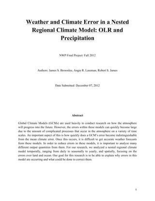
  • 8. 8 3.2) Error Growth Fig. 6 depicts the error growth of precipitation in the model domain. A calculation of precipitation RMSE for each individual day for the month of January 1996 and the average climate precipitation root mean squared error over the entire 5-year simulation is shown in Fig. 6. The purpose of this image is to analyze how soon after model initialization does the precipitation errors match up to the mean climate error. Using this method, our results show that our NRCM took approximately seven days the for precipitations errors to catch up to the mean climate error, calculated over the entire five-year period, and seemed to oscillate around that mean for the remainder of the month of January. The usage of the model for forecast purposes on any given day after 8 January 1996 would have yielded very inaccurate results, and thus the error seen in the climatological mean would be just as good, if not better, than the forecast output from this NRCM. In order to receive accurate precipitation forecasts and creating forecasts, it would be necessary to run the model at least every 7 days in order to achieve lower forecast errors than the climatological average. Since the only available initialization time for our study was 1 January 1996, we are unable to see if this is a continuous error in this model if it was able to be initialized more often, or if there was another underlying issue causing the RMSE to rise so quickly. To determine this we would need to be able to initialize this model and numerous times to see if the error is reoccurring. During this process it would also be necessary to see how it changes based on the time of initialization, instead of only having output on a daily time scale. 4) Comparison of Precipitation Error to Outgoing Longwave Radiation 4.1) Background on Outgoing Longwave Radiation Techniques
  • 9. 9 In this section of the paper, an analysis of the relationship between outgoing longwave radiation (OLR), cloud cover, and precipitation intensity will be carried out over the domain that is described in the introduction section. However before getting into the analysis of these results, some background on this subject area is needed. Since 1974, NOAA’s polar orbiting satellites have been making estimates of OLR (Hartmann and Recker 1986; Xie and Arkin 1998). This continual input of OLR data has been used in many different meteorological studies. One very large and prominent area of research in this field has focused on OLR trends over the tropics. Since there is little variation in temperature over the tropics, any significant changes in OLR are generally caused by changes in cloud cover. Since the early 1980s, OLR has been used to quantitatively estimate precipitation, and many studies have made use this technique; this technique has proven to be a very accurate way to remotely estimate precipitation (Xie and Arkin 1998; Liebmann 1998). Some examples of how this technique is applied in studies will be shown in the following examples. Markin and Meisner (1987) used a Geostationary Operational Environmental Satellite (GOES) Precipitation Index (GPI) to study the correlation between values of OLR and precipitation over different regions of the tropics. In their study, they found that low values of OLR correlated with larger amounts of precipitation (Markin and Meisner 1987; Xie and Arkin 1998). In a 1991 study, Janowiak and Arkin developed an equation, using statistical techniques, which could estimate precipitation based on values of OLR. The techniques used in these studies considered the total flux of OLR. Deep convective clouds largely control this flux over the tropics because there is little variation of temperature over such regions of the planet (Xie and Arkin 1998). Such techniques cannot be used in the same manner over the middle latitudes because there are larger changes in temperature; these changes in temperature also regulate the
  • 10. 10 OLR flux, and not solely dependent on changes in cloud coverage. In their 1998 study, Xie and Arkin investigated what the correlations are between global OLR values and precipitation intensities. In their study, they found a strong relationship between low values of OLR and high precipitation rates of the tropical regions. Over the middle latitude regions, the cloud coverage- OLR relationship was not as clearly defined because as stated above, the influence of temperature changes also controls changes the overall OLR flux. Trends in OLR can also be used to study the decadal shifts in convection over the tropics. In their 1997 study, Chu and Wang used statistical methods to study the changes in overall convection that occurred from 1974-1992. In their study, they found that over the last several years, OLR values had greatly decreased over the West Central Pacific, over the Indian Ocean, and over the Bay of Bengal. This was attributed to an overall increase in convective rainfall in this region, and this increase in rainfall was primarily attributed to a gradual strength in the monsoon. Over this same period, OLR values increased over Australia, signifying a decrease in rainfall (Chu and Wang 1997). So, in summary, these studies clearly show that OLR values can be used to study convective rainfall patterns over the tropical belt. Now that some background on this subject has been covered, the current analysis of OLR and precipitation over the tropical belt can be carried out. 4.2) Precipitation Error Correlated to OLR Fig. 7 shows the overall five-year average of satellite observed OLR values starting on 1 January 1996 and ending on 31 December 2000. Also shown in this figure is the difference between the five-year average of observed precipitation amounts and the five-year average model precipitation amounts. The five-year averaged model precipitation is the sum of both convective and non-convective rainfall. The trend in precipitation in this figure is similar to Figs.
  • 11. 11 2, 3, and 4. The NRCM WRF model overestimated rainfall over regions with large amounts of precipitation, and it underestimated precipitation in dry regions. So, it could be said that the model is positively biased towards regions with increased rainfall, and negatively biased towards regions with little rainfall. These positive and negative biases towards regions of high and low precipitation have been observed in other model studies, particularly for those where a nested regional climate model was used (Liu et al. 2012; Murthi et al. 2010). So, in summary, the model overestimates precipitation in regions with high rainfall and the model underestimates precipitation in regions with little rainfall. Despite these biases, the models output clearly does show a strong correlation between high precipitation regions and outgoing longwave radiation. In Fig. 7, the regions with the highest precipitation contain the lowest values of OLR. In contrast, the regions with little precipitation have much higher values of OLR. Over the Indian Ocean, the OLR values are quite low, and in this region the model output depicts higher precipitation. This also occurs along the ITCZ, over Central Africa, and over northwestern South America. As shown in Figs. 9 and 10, the model output shows that convective precipitation dominates in these regions. It is likely that the model is overestimating the amount of convective precipitation over the tropical regions, especially over the ocean. A more in depth discussion of this potential error will occur later on this section of the paper. Over Australia and Northern Africa the OLR values are much higher, and as shown in the model output, there is little precipitation in these regions. In addition to that, the model output suggests that there is almost no convective precipitation in these drier regions. Previous research shows that OLR flux within the tropical belt is mostly controlled by convective clouds, (Xie and Arkin, 1998; Markin and Meisner, 1987) and this trend is clearly shown in Fig. 6. The OLR is much lower in regions where there is a local maximum in rainfall
  • 12. 12 and vice versa. So, despite the models bias towards dry and wet regions, the model output when plotted with satellite derived OLR data, clearly shows the correlation between convective cloud cover and OLR values. The regions with lower OLR values correlate with higher amounts of convective rainfall, and the regions with higher OLR have little precipitation and almost no convective rainfall. 4.3) Seasonal OLR Analysis Fig. 8 shows the five-year seasonal average of OLR from 1 January 1996 to 31 December 2000. Each of the five-year OLR averages are taken over three month periods, the first being March, April, and May (Northern hemisphere spring); the second being June, July, and August (Northern hemisphere summer); the third being September, October, and November (Northern hemisphere fall); and the fourth being December, January, and February (Northern hemisphere winter). Similar to Fig. 7, the regions with low OLR values correlate with higher precipitation rates (Markin and Meisner, 1987). There are several interesting trends that can be deciphered within these seasonal precipitation patterns. First, during all four seasons, the OLR data clearly displays the ITCZ over the tropical belt. In addition to that, during the March, April, and May time period, the heaviest precipitation occurs over the northern part of South America, over Central Africa, and over the island chains in the central part of the Western Pacific Ocean. By June, July, and August, the rainfall area decreases over South America, and it increases greatly over the central part of the Western Pacific and Northern Indian Oceans. Also, the rainfall increases over the eastern part of the Central Pacific. During the September, October, and November time period, rainfall remains heavy over the Indian Ocean and over the West Central Pacific, and it increases over the western part of South America. Secondly, precipitation remains significant over Central Africa. Over the December, January, and February time period, rainfall
  • 13. 13 increases southward over Central Africa and Central South America; the rainfall belt also shifts slightly southward over the West Central Pacific moving towards Australia. There are many global and regional oscillations in the atmosphere and ocean that are responsible for these seasonal shifts in OLR and rainfall over the tropics. In the next part of this section, some explanations will show how these seasonal patterns cause the observed seasonal shifts in OLR and rainfall will be attempted, with the primary focus being on the Central Eastern Pacific, Central South America, and the Northern Indian Ocean. The large area of negative OLR values observed over South America during the December to February time period (Southern hemisphere summer) is primarily driven by the convergence that occurs along the South Atlantic Convergence Zone (SACZ) and along the ITCZ (Nogues-Paegle and Mo, 1997; Liebmann et al 1999). This large area of clouds and precipitation continues through the March to May time period. By the time Southern hemisphere winter (June to August) comes, the ITCZ has moved northward and the SACZ has weakened, thus there is noticeable increase in OLR over Central South America due to decreased rainfall and cloud coverage. The next area of interest is over the central part of the Eastern Pacific Ocean. Of interest here is whether or not the large El Nino that occurred at the end of 1997 and at the beginning of 1998 is discernible over the five-year average of seasonal OLR values. From the Northern hemisphere spring to summer there is a large decrease in OLR values over the central part of the Eastern Pacific, indicating an increase in sea surface temperatures (SSTs) and deep convection. From summer to fall, the five-year averaged values of OLR slightly increase, indicating that the convection has weakened slightly. By winter, the OLR values indicate little to no convection over this region. In their 2000 study, Wang and Weisberg, analyzed the different changes in
  • 14. 14 atmospheric and oceanic anomalies that occurred during the development and decay of the 1997/1998 El Niño event. In their study, they found that values of OLR began to decrease over the Central Eastern Pacific between July and September of 1997. During the main stage of the El Niño, which went from December of 1997 to January of 1998, there was large area of negative OLR values of the central part of the Eastern Pacific, signifying that widespread deep convection was occurring over the area during that time. This large area of convection persisted into the February to April of 1998 time period (Wang and Weisberg, 2000). Comparing this pattern to the five-year average values of OLR in Fig. 7 suggests that any signal from the 1997/1998 El Niño is not even noticeable over the five-year seasonal averages. OLR values greatly decreased from July of 1997 to December of 1997 during the developing El Nino event, while over the five-year average period, OLR values decrease from summer to winter. Again this suggests that the El Niño signal is not detectable over the five-year average in observed OLR values. Lastly, it should be noted that it is possible that the strong convective precipitation estimates in the model output within Figs. 9 and 10 could have been influenced by the 1997/1998 El Niño event, however such an assumption is at best inconclusive. Over the Northern Indian Ocean, the Indian Monsoon controls the seasonal variations in convection. The monsoon is marked by widespread deep convection over the northern Indian Ocean during the summer period, especially over the Bay of Bengal (Sengupta and Ravichandran, 2001). In addition to that, convection is enhanced over the eastern part of the Northern Indian Ocean (Gadgil et al. 2003). This pattern is clearly evident in the 5 year averaged OLR values over the Bay of Bengal. The lowest OLR values occur during the Northern Hemisphere Summer; this is when convection is most enhanced over the Bay of Bengal region. Clearly, the five-year
  • 15. 15 averaged OLR values over the Northern Indian Ocean are largely controlled by the seasonal Indian Ocean monsoon pattern. 5) Convective and Non-convective Precipitation Figs. 9 and 10 show the five-year average in the areal extent of convective and non- convective precipitation over the tropical belt from 1 January 1996 to 31 December 2000. Previous research has shown that when sampling the real atmosphere, amounts of convective and non-convective precipitation should be roughly equal (Gamache and Houze, Jr. 1983; Houze, Jr. and Rappaport 1984). In Fig. 9, the model output shows that there is whole lot more convective precipitation over the tropics then there is non-convective/stratiform precipitation. In Fig. 10, it is again clear that the precipitation in the model output is dominated by convective precipitation. It is likely that the model has greatly overestimated the areal extent of precipitation that is convective and underestimated the areal extent of precipitation that is stratiform. Studies have shown that over the tropics, especially in the oceanic regions, rainfall mainly comes from mesoscale convective cloud systems (Waliser and Graham, 1993; Schumacher and Houze, 2003). Within in these convective systems there are three main components: deep convective towers at the front of the cloud system which release large amounts of latent heat, a large area of trailing stratiform precipitation, and a large cirrus cloud shield near the tropopause (Waliser and Graham, 1993). The structure of these mesoscale convective systems is common to both tropical and non- tropical mesoscale convective systems (Rutledge et al. 1988; Ely et al. 2008). Based on the above description of these tropical convective systems, there is clearly both convective and stratiform precipitation occurring within these systems. However, the stratiform precipitation covers a much larger area then the convective precipitation that occurs at the front of the cloud system. This means that when the average of all these systems is summed up, there should be an
  • 16. 16 overall larger area of stratiform precipitation over the tropics, it turns out that studies confirm this. Schumacher and Houze (2003) used the Tropical Rainfall Measuring Mission (TRMM) Precipitation Radar over the years of 1998-2000 to estimate the amount of convective and non- convective precipitation over tropical regions. They found that 73% of the areal extent in precipitation was covered by stratiform rainfall, but it only accounted for 40% of the total rainfall during the three-year period (Schumacher and Houze, 2003). An older study in 1996, similarly found that 74% of the precipitation in the tropics was stratiform, and the remaining 26% percent was convective precipitation (Tokay and Short, 1996). Based off these studies, it is clear that the model used in this study has underestimated the areal extent of stratiform precipitation. Most of the model output shows only convective precipitation over the tropics and very little stratiform precipitation. This means that this model has greatly overestimated the areal of extent of stratiform precipitation over the tropics, especially over the Central Western North Pacific and Northern Indian Ocean. It is possible that this regional model is having a hard time capturing the small-scale processes that drive these mesoscale convective systems. This model has a horizontal resolution of 36 km, so its resolution is not high enough to capture the convective scale processes that occur within the cloud systems. Studies have shown that decreasing the resolution of the regional model down to a few kilometers or a few hundred meters is the best way to accurately portray convective systems (Bryan et al. 2003; Lean et al. 2008; Kalnay p.12). Since this model was run at a horizontal resolution of 36 km, it is likely having trouble in distinguishing the difference between convective and non-convective precipitation within the mesoscale cloud systems. So perhaps the coarse resolution of this WRF model is one reason why the model is greatly underestimating the areal extent of stratiform precipitation in the tropics.
  • 17. 17 6) Zonal and Meridional Averages Fig. 11 shows the zonal (west to east) five-year model output average of convective precipitation, non-convective precipitation, and observed OLR values from 30°S to 30°N. As with the other figures in this report, the time goes from 1 January 1996 to 31 December 2000. This figure clearly shows the correlation between values of OLR and the amount of convection, which occurs at each zonal average. At between 5°N and 10°N, the convection is at its strongest. This large maximum five-year zonal average in convection is clearly being caused by the tropical rain belt/ITCZ. When the convection is at its maximum value, OLR values are at a minimum. This figure again shows that when there is lots of cloud cover and convection, OLR values are quite low. OLR values and non-convective precipitation do not appear to be correlated; it is primarily dominated by convective precipitation. As discussed earlier, this model is likely overestimating the areal extent of convective precipitation over the tropics. Fig. 12 displays the meridional (North to South) five-year model output average of convective precipitation, non-convective precipitation, and observed OLR values starting and ending at the Prime Meridian. In other words, this figure shows the meridional average across the entire globe. There are two average maximums in convective activity that occur in this figure. The first is at roughly 60° W. At this longitude, there is a large amount of equatorial convection in South America, and this is contributing to the meridional average maximum in Fig. 12. As expected, at this longitude, values of OLR are at a minimum. The second and much stronger maximum in convective activity occurs from longitudes 60°E to 160°E. Most of this maximum in convection is due to the monsoon that occurs over the Northern Indian Ocean and the large warm pool that occurs over the Central Western Pacific Ocean. So, this figure shows that on average, the strongest and most persistent convection occurs over the Northern Indian Ocean and
  • 18. 18 the Central Western Pacific; other studies have also shown that this region generally has the largest areal coverage of intense convection over the tropics (Gettelman et al. 2002). Again it should be noted, that according to this model output, the non-convective precipitation is not well correlated with values of OLR, the model output is dominated by convective precipitation. 7) Conclusion Our research shows that the NRCM used has high amounts of convective precipitation over a large majority of its domain due to convective parameterization within the coarse resolution of this model. We analyzed how model errors differed between various temporal scales, and what meteorological and climatological features could have resulted in these errors. Some of the errors found within the model can be correlated to the observed OLR data over the same time period. ENSO was found to be a key factor in some of the model errors when looking at yearly averages from 1996 to 2000, as an El Niño event occurred during 1997 and 1998 and can be seen in some of the error fields in Fig. 3. When trying to use this model to predict precipitation amounts into the future, we found that this model is very poor and its errors are roughly equal to the mean climate error approximately seven days after initialization. In order to minimize the model’s weather error, it would need to be run at least every seven days for accurate weather forecasts to be made. The NRCM also has large errors associated with its convective parameterization scheme, which it relies on heavily being a coarse resolution model. We created Fig. 9 to show the large discrepancy the model has between amounts of convective and non-convective precipitation. Similar to precipitation errors, zonal and meridional averages of convective precipitation, studied in Figs. 11 and 12, were found to also correlate well to observed OLR values. Areas that observed lower amounts of OLR also experienced a rise in the
  • 19. 19 amount of convective precipitation, while areas with higher amounts of OLR experienced a decrease in the amount of convective precipitation. Overall, we feel that this model is not a great estimator of the climate throughout its domain and needs to be improved. In addition, its ability to forecast weather conditions does not seem viable after approximately seven days after initialization.
  • 20. 20 Fig. 1. Zonal domain of the NRCM used in this research. The red box denotes the approximate domain in which our research focuses, from 30°S to 30°N and 0°W to 360°W.
  • 21. 21 Fig. 2. Seasonal error of model output (sum of convective and non-convective precipitation) and observations (total rain) between 1996 and 2000 with units of mm day-1 . Positive values correlate to model overestimation.
  • 22. 22 Fig. 3. Annual error of model output (sum of convective and non-convective precipitation) compared with observations (total rain) between 1996 and 2000 with units of mm day-1 . Positive values correlate to model overestimation of precipitation.
  • 23. 23 Fig. 4. Mean climate error of model output (sum of convective and non-convective precipitation) compared with observations (total rain) between 1 Jan 1996 and 31 Dec 2000 with units of mm day-1 . Positive values correlate to model overestimation. Fig. 5. Root mean squared error (RMSE) of model output (sum of convective and non- convective precipitation) compared with observations (total rain) between 1 Jan 1996 and 31 Dec 2000.
  • 24. 24 Fig. 6. Calculation of precipitation RMSE (sum of convective and non-convective) for each individual day for the month of January 1996 (blue line), and the average climate precipitation RMSE over the entire 5-year simulation (red line). Fig. 7. Average OLR (shaded, W m-2 day-1 ) and a difference field of modeled (sum of convective and non-convective precipitation) and observed precipitation (see Figure 3, contoured, mm day-1 ) over the period of 1 Jan 1996 to 31 Dec 2000. Positive values of the difference field correspond to the solid contours; negative values correspond to dashed contours
  • 25. 25 Fig. 8. Seasonal average of OLR (W m-2 day-1 ) between 1996 and 2000.
  • 26. 26 Fig. 9. Model output of (a) convective and (b) non-convective precipitation, averaged over the time period of 1 Jan 1996 to 31 Dec 2000. Filled contours have units of mm day-1 .
  • 27. 27 Fig. 10. Difference of the average model output of convective and non-convective rain. Positive values (red colors) correlate to a larger convective rain average.
  • 28. 28 Fig. 11. Zonal average of (a) convective, (b) non-convective modeled precipitation (units of mm day-1 ), and (c) OLR (units of W m-2 day-1 ) for the period of 1 January 1996 to 31 December 2000.
  • 29. 29 Fig. 12. Meridional average of (a) modeled precipitation (convective, black line; non-convective, red line), and (b) OLR (units of W m-2 day-1 ) for the period of 1 January 1996 to 31 December 2000.
  • 30. 30 References Allen, M., J. Kettleborough, D. Stainforth, 2006: Model error in weather and climate forecasting. Predictability Wea. Clim. Cambridge University Press, 718 pp. Arkin, P. A., and B. N. Meisner, 1987: The relationship between large scale convective rainfall and cold cloud over the Western Hemisphere during 1982-84. Mon. Wea. Rev., 115, 51-74. Bryan, G. H., and J. C. Wyngaard, 2003: Resolution requirements for the simulation of deep moist convection. Mon. Wea. Rev., 131, 2394-2416. Chambers, D. P., B. D. Tapley, R. H. Stewart, 1999: Anomalous warming in the Indian Ocean coincident with El Niño. J. Geo. Res., 104, 3035-3047. Chu, P. S., and J. B. Wang, 1997: Recent climate change over the tropical Western Pacific and Indian Ocean regions as detected by outgoing long wave radiation records. J. Climate, 10, 636- 646. Ely, B. L., R. E. Orville, L. D. Carey, and C. L. Hodapp, 2008: Evolution of the total lightning structure in a leading-line, trailing-stratiform mesoscale convective system over Houston, Texas. J. Geophys. Res., 113, D08114, doi:10.1029/2007JD008445. Gadgil, S., P. N. Vinayachandran, and P. A. Francis, 2004: Extremes of the Indian summer monsoon rainfall, ENSO and equatorial Indian Ocean oscillation. Geophys. Res. Lett., 31, L12213, doi:10.1029/2004GL019733. Gamache, J. F., and R. A. Houze, Jr., 1983: Water budget of a mesoscale convective system in the tropics. J. Atmos. Sci., 40, 1835-1850. Gettelman, A., M. L. Salby, and F. Sassi, 2002: Distribution and influence of convection in the tropical tropopause region. J. Geophys. Res., 107, doi:10.1029/2001JD001048. Hartmann, D. L., and E. E. Recker, 1986: Diurnal variation of outgoing longwave radiation in the tropics. J. Climate Appl. Meteor., 25, 800-812. Houze, R. A., Jr., and E. N. Rappaport, 1984: Air motions and precipitation structure of an early summer squall line over the eastern tropical Atlantic. J. Atmos. Sci., 41, 553-574. Janowiak, J. E., and P. A. Arkin, 1991: Rainfall Variations in the tropics during 1986-1989, as estimated from observations of cloud top temperature. J. Geophys. Res., 96, 3359-3373.
  • 31. 31 Janowiak, J. E., P. A. Arkin, P. Xie, M. L. Morrissey, and D. R. Legates, 1995: An examination of the East Pacific ITCZ rainfall distribution. J. Climate, 8, 2810-2823. Kalnay, E., 2003: Atmospheric Modeling, Data Assimilation and Predictability. Cambridge University Press, 341 pp. Lean, H. W., P. A. Clark, M. Dixon, N. M. Roberts, A. Fitch, R. Forbes, C. Halliwell, 2008: Characteristics of high-resolution versions of the met office unified model for forecasting convection over the United Kingdom. Mon. Wea. Rev., 136, 3408-3424. Liebmann, B., J. A. Marengo, J. D. Glick, V. E. Kousty, I. C. Wainer, and O. Massambani, 1998: A comparison of rainfall, outgoing long wave radiation and divergence over the Amazon Basin. J. Climate. 11, 2898-2909. Liebmann, B., G. N. Kiladis, J. A. Marengo, T. Ambrizzi, and J. D. Glick, 1999: Submonthly convective variability over South America and the South Atlantic Convergence Zone. J. Climate, 12, 1877–1891. Liu, L., P. A. Richard, and G. J. Huffmen, 2012: Co-variation of temperature and precipitation in CMIP5 models and satellite observations. Geophys. Res. Lett., 39, doi:10.1029/2012GL052093. McPhaden, M. J., and Coauthors, 1998: The tropical ocean-global atmosphere observing system: A decade of progress. J. Geo. Res., 103, 14169-14240. Murthi, A., K. P. Bowman, and L. R. Leung, 2011: Simulations of precipitation using NRCM and comparisons with satellite observations and CAM: annual cycle. Clim. Dynamics, 36, 1659- 1679. Nogués-Paegle, J., and K. C. Mo., 1997: Alternating wet and dry conditions over South America during summer. Mon. Wea. Rev., 125, 279–291. Rasmusson, E. M., T. H. Carpenter, 1983: The relationship between eastern equatorial pacific sea surface temperatures and rainfall over India and Sri Lanka. Mon. Wea. Rev., 111, 517–528. Rasmusson, E. M., and J. M. Wallace. "Meteorological aspects of the El Niño/Southern Oscillation." Science 222.4629 (1983): 1195-1202. Richardson, C. W., Stochastic simulation of daily precipitation, temperature, and solar radiation. Water Resources Res., 17, 182-190.
  • 32. 32 Ropelewski, C. F., and M. S. Halpert, 1996: Quantifying Southern Oscillation-precipitation relationships. J. Climate, 9, 1043-1959. Ropelewski, C. F., and M. S. Halpert, 1987: Global and regional scale precipitation patterns associated with the El Niño/Southern Oscillation. Mon. Wea. Rev., 115, 1606-1626. Rutledge, S. A., P. V. Hobbs, R. A. Houze Jr., M. I. Biggerstaff, and T. Matejka, 1988: The Oklahoma–Kansas mesoscale convective system of 10–11 June 1985: Precipitation structure and single-Doppler radar analysis. Mon. Wea. Rev 116: 1409-1430. Schumacher, C., and R. A. Houze Jr., 2003: Stratiform rain in the tropics as seen by the TRMM precipitation radar. J. Climate. 16, 1739-1756. Sengupta, D., and M. Ravichandran, 2001: Oscillations of Bay of Bengal sea surface temperature during the 1998 summer monsoon. Geophys. Res. Lett., 28, 2033-2036. Thornton, P. E., and S. W. Running, 1999: An improved algorithm for estimating incident daily solar radiation from measurements of temperature, humidity and precipitation. Ag. Forest Met. 93, 211-228. Tokay, A., and D. A. Short, 1996: Evidence from Tropical Raindrop Spectra of the Origin of Rain from Stratiform versus Convective Clouds. J. Appl. Meteor., 35, 355–371. Trenberth, K. E., 1997: The definition of El Niño. Bull. Amer. Meteor. Soc., 78, 2771–2777. Waliser, D. E., and N. E. Graham, 1993: Convective cloud systems and warm-pool sea surface temperatures: Coupled interactions and self-regulation. J. Geophys. Res., 98, 12881-12893. Waliser, D. E., and C. Gautier, 1993: A satellite-derived climatology of the ITCZ. J. Climate, 6, 2162-2174. Wang, C., R. H. Weisberg, 2000: The 1997–98 El Niño evolution relative to previous El Niño events. J. Climate, 13, 488–501. Wilks, D. S., 1995: Statistical Methods in Atmospheric Sciences. Academic Press, 467 pp. Williamson, G. B., W. F. Laurance, A. A. Oliveira, P. Delamônica, C. Gascon, T. E. Lovejoy, and L. Pohl, 2000: Amazonian tree mortality during the 1997 El Niño drought. Cons. Bio., 14, 1538-1542.
  • 33. 33 Winslow, J. C., E. R. Hunt Jr., 2001: A globally applicable model of daily solar irradiance estimated from air temperature and precipitation data. Eco. Modeling, 143, 227-243. Wu, X., X. Z. Liang, G. J., Zhang 2003: Seasonal migration of ITCZ precipitation across the equator: Why can't GCMs simulate it? Geophys. Res. Lett., 30, 1824-1828. Xie, P., and P. A. Arkin, 1998: Global monthly precipitation estimates from satellite observed outgoing longwave radaition. J. Climate. 11, 137-164.