SlideShare a Scribd company logo
1 of 43
Download to read offline
THE PROJECT OF THE RED BLOOD CELL
APPLYING THE RECENT STUDY TO DERIVE AN ANCHOR-RING RBC MODEL
A PROJECT
Presented to the Department of Mechanical and Aerospace Engineering,
California State University, Long Beach
In Partial Fulfillment
Of the Requirements for the Degree
Master of Science in Mechanical Engineering
By Hung-Wen Huang
B.S., 2002, Northern Taiwan Institute of Science and Technology,
Taipei, Taiwan
December 2008
iv
TABLE OF CONTENTS
Page
ACKNOWLEDGEMENTS ……………………………………………………….. iii
LIST OF TABLES …………………………………….……………………….…… v
LIST OF FIGURES …………………………………………………………..……. vi
Introduction .......................……..…..............................................……………......... 1
Previous Experimental Researches for the RBC ..….............................….………… 1
Previous Mathematical Models and Analytical Solutions .…........….…………....... 6
Recent Study of the Anchor-Ring Vesicle Red Blood Cell .....…………….............. 10
Finding the Compatibility Equations ..…………............…………........................... 13
Procedure of Solving the Equations ..………….................………............................ 16
MATLAB Codes....……………………..…......... ..………….…............................... 18
Running an Example ……………......…………………............................................. 19
Inspection of the Result ..........………………………………..........…....................... 23
Final Results ........……….....................….............................…………….................. 23
Possible Improvement in the Future ........…………….............................……….….. 29
Summary ......................................................…………………….………..……….... 33
Reference ...................................…............………………………………..……….... 35
Appendix A .............................….……………....…………………..……….……… 37
Appendix B ..........................…….….…………………………………..…………… 38
Appendix C .............................……………..………………..……….……………… 39
v
LIST OF TABLES
TABLE Page
1. Valid Ranges for λ , p∆ , ck , and ρ ………….…………………….…… 19
2. The First result after running RK4 ………….…………………...…….…… 22
3. Final values for λ , p∆ , ck , ρ , a and c0 ………….…………………..… 24
vi
LIST OF FIGURES
FIGURE Page
1. Cross-Sectional Shape of the Average RBC and other
Geometrical Data ……………………………………………………...……. 3
2. Three fundamental 3D RBC Models ………….……….………...…….…… 4
3. Different Shapes of RBC ……………………………..…………………..… 5
4. Human Red Blood Cell Membrane Structure ……………………………… 7
5. The cross section of a ring vesicle with generating radii …………………... 9
6. The coordinate system of RBC’s quarter cross-section ……………………. 12
7. The flow chart for solving the differential equation ……………………….. 18
8. The first result for testing the codes …………………………………….…. 22
9. The quarter cross-section of the final result ……………………………….. 24
10. The full cross-section of the final result …………………………………. 25
11. The full 3D model of the final result of the RBC shape equation
(i.e. Eq.5 and Eq.6) ………………………………………………………... 26
12. The cross-section of the 3D model of the RBC shape equation
(i.e. Eq.5 and Eq.6) ………………………………………………………... 27
13. The cross-section and coordinate system of a biconcave-
discoid model ………………………………………………………………. 31
14. The full cross-section of the biconcave- discoid model which is
derived from Zhou’s shape equation ……………………………………….. 32
1
Introduction
The Red Blood Cell (RBC) is one of the most common blood cells in our body. From
many previous research results, several RBC proprieties such as shape, dimension, and
osmotic pressure can now be determined by experiments with precise measurements. In
addition, there are several physical and mathematical models of the RBC that were
proposed by some biophysics pioneers. However, since finding the analytical solutions of
these RBC models involves a high complexity and nonlinearity, it requires further study
and research. The purpose of this project is to find the geometrical solutions for one of
the most recent study of the RBC, namely, solutions of the shape equation proposed by
Zhou [1]. The project focuses on the anchor-ring RBC [2]. By accessing several
mechanical properties such as osmotic pressure, bending module, and tensile stress, the
close form solutions were obtained, and the results are examined and verified with
previous experimental studies.
Previous Experimental Researches for the RBC
Fung and Evan are two of the most important scholars in bioengineering. In their
previous work about the measurement of the RBC [3], they proposed an improved
method of measurements for RBC. According to Fung and Evan, dimensions of an object
in the living state such as a RBC are the keys of solving problems in biophysics. Also,
dimensions are the most important factors to determine what an object’s shape would be.
Thus, the measurements accuracy is very important before one can determine the shapes
of RBCs. However, measuring dimensions of the RBC with traditional or normal micro
measurement would present some limitations since the dimensions of the RBCs are too
2
small to be comparable with the light wavelength. Nevertheless, observing a RBC is such
a challenge due to its physical weakness. For example, when researchers wish to study
the elasticity of the RBC, they must observe the specimen under stress and strain,
whereas there will be a tremendous chance to spoil RBC’s biophysical properties because
the stress-and-strain relationship of RBC can be easily altered by fixation or radiation.
Thus, Fung and Evan processed the optical image through an interference microscope to
obtain a higher resolution of the image which could mitigate the problem and obtain the
further accuracy from the measurements of RBC. The results was recorded and produced
based on three different statistics conditions (RBC at 300, 217, and 131 milliosmoles
(mOsm), a unit of osmotic pressure that could be converted to other common pressure
unit. One osm is the osmotic pressure of a one molar solution, i.e. 1 mole/L of solvent).
Then, the three average shapes of RBC’s cross sections from the tonicity can be described
as shown in Figure 1 [3]. From Figure 1, several parameters of RBC’s geometry are
revealed. The diameter of RBC from tonicity is approximately between 6.78 and 7.82 Ӵ
m. The volume is from 94 to 164 Ӵm3, and the surface area is from 135 to 145Ӵm2.
Figure 1 shows the cross-sections of all three basic types of RBC shapes. By revolving
each cross-section shape with each central axis, three RBC shapes can be generated by
3D plotting as shown in Figure 2 [1]. Beside these three basic shapes, there are still
several mutations. As shown in Figure 2, the type of 300 and 217 mO are described as a
biconcave-discoid model. In fact, several variations of RBC shapes could exist due to
different environments and conditions.
3
Figure 1. Cross-Sectional Shape of the Average RBC and other Geometrical Data.
7.82 Ӵ̀
Volume = 94 Ӵ̀
 
Surface Area = 135 Ӵ̀
¡
300 mO
7.59 Ӵ̀
Volume = 116 Ӵ̀
 
Surface Area = 135 Ӵ̀
¡
217 mO
6.78 Ӵ̀
Volume = 164 Ӵ̀
 
Surface Area = 145 Ӵ̀
¡
131 mO
4
Figure 2. Three fundamental 3D RBC Models.
According to Gov, N. [4], altering the difference in osmotic pressure between the outside
and inside environment could cause the changes in RBC shape. This could result in
RBC’s geometric shape change into a swollen or crenated type. Moreover, altering the
structure of the underlying membranous cytoskeleton could also change RBC’s shape.
Figure 3a [5] shows the shapes of RBC inconsistently exist compared to the three
standard types while they are enduring different physical and biological conditions in our
bodies. In Figure 3b [5], both closed standard shape (left one) and the swollen shape
(right one) are shown. Figure 3c [5] indicates the existence of the nearly spherical shape.
In addition, a serious variation is shown in Figure 3d [5]. It is called an anchor-ring
vesicle without the membrane in the middle.
300 mO 217 mO131 mO
5
Figure 3. Different Shapes of RBC.
6
Previous Mathematical Models and Analytical Solutions
For several decades, researchers have attempted to find out the analytical solutions to
describe the RBC’s physical and geometrical properties. In 1973, Helfrich [6] proposed
an energy equation that could determine the equilibrium shape of a vesicle by minimized
the free curvature energy, namely shape energy [2, 6]. The equation is shown below:
( ) +∆+−+= dAdVpdAccckF c λ2
0212
1
, (1)
where,
ck is the bending module (elastic constant).
1c and 2c are two principal curvatures.
0c is the spontaneous curvature of the vesicle membrane surface.
10 ppp −=∆ is the osmotic pressure difference between outer and inner media.
λ is a tensile stress acting on the membrane.
The Helfrich’s energy equation becomes the most significant analytical foundation of the
recent studies for RBC shapes. As a result, four of the above parameters ( ck , 0c , p∆ , λ )
become key factor in the BC studies. Therefore, understanding those parameters would be
the first step to investigate analytical solutions of RBC shapes. First of all, the parameter
ck represents the bending rigidity of the vesicle membrane. It is used as an elastic
constant to indicate the stiffness of the vesicle. The range of RBC’s bending module ( ck )
is between 9
107.1 −
× to 19
107 −
× (N.m) [7]. p∆ is the difference of the osmotic
pressure between RBC’s inner and outer media with the values between 65 to 140 N/m2
7
[7]. λ can be dynamic or static. This project studies the static case only, so the range of
λ is between 6
102 −
× to 6
106 −
× [8]. The RBC’s membrane structure is very complex.
It is constructed by lipid bilayers, spectrin network, and transmembrane proteins [4]. As
shown in Figure 4 [4], there could be many vacancies and uniform
Figure 4. Human Red Blood Cell Membrane Structure.
structures in RBC’s membrane, so it is very difficult to describe the detail of this
phenomenon. Thus, Helfrich [6] defined the spontaneous curvature ( 0c ) in the
mathematical model as a parameter to adjust the practical difference. Although 0c
usually appears as an unknown constant in the equation, it could be determined when the
boundary conditions and experimental data can be found though the process of solving
the differential equation. Therefore, finding 0c became the first important work of this
project. In 1987, Ou-Yang Zhong-Can, a theoretical physicist in crystal solid physics and
8
optics in China, and Helfrich derived the general shape equation (OH General Shape
Equation) based on Helfrich’s spontaneous curvature theory as follows [2, 9].
02))((42 2
02
12
02
1
=∇+−−++−∆ HkHcKHcHkHp ccλ , (2)
where 2
∇ denotes the Laplacian operator. H is the mean curvature, and K is Gauss
curvature. Unlike Helfrich’s energy equation, the OH general shape equation further
improves the use of ∆ p and λ without just considering those two parameters as
Lagrange multipliers. According to Ou-Yang [2], the various solutions of Eq.2 are
calculated by numerical methods under the assumption of the azimuthal symmetry and
topological spheres. He attempted to introduce the ring functions or toroidal functions
into certain aforementioned parameters [10]. Ou-Yang defined the name of the vesicle’s
shape for a further genus (besides those with spherical topology) as an anchor ring. Then,
transferred the mean curvature H, the Gauss curvature K, and the term 2
∇ H into the
hyperbolic and trigonometric functions. After plugging those hyperbolic and
trigonometric functions of the mean curvature, Gauss curvature, and 2
∇ H back into Eq.2,
certain coefficients are obtained, and it shows that the generating circles have the radii
with ratio 2/1 in the anchor-ring vesicles of RBC. Also, these rings are stable for
negative values of the spontaneous curvature 0c which satisfies
9.3)4/2()2( 2
32/1
00 −≈+−< πrc . (3)
According to Ou-Yang, since the mechanical equilibrium equation of vesicle membranes
9
(Eq.2) is highly nonlinear, it is not an easy task to find exact and analytic solutions. So far,
besides the case of a sphere, no analytical solution is known yet. Based on the result of
what Ou-Yang had found, Mutz and Bensimon made an observation of RBC’s toroidal
vesicles and found an agreement with Ou-Yang’s theory [11]. They tried to measure the
dimension of the outer diameter (D) and the width (d) of the ring vesicle as shown in
Figure 5 [11].
Figure 5. The cross section of a ring vesicle with generating radii. D represents the outer
diameter and d is the width of the ring.
Their observation reveals the mean ratio between the outer diameter D and the width d is
02.041.0 ± which is in good agreement with the theoretical prediction proposed by
Ou-Yang [2] (i.e. 12 − , the appropriate value for the ratio of the diameters).
10
Recent Study of the Anchor-Ring Vesicle Red Blood Cell
In the studying of mathematical model for RBC shapes, three important shape equations
were developed. They are Deuling and Helfrich (DH) Shape Equation, Seifert, Berndl
and Lipowsky (SBL) Shape Equation, and Hu and Ou-Yang (HO) Shape Equation [1].
The first two were developed based on Helfrich’s spontaneous curvature theory and
energy, and the last one was derived based on OH equation (Eq.2) [12]. According to a
recent study [1], general analytical solutions of these shape equations are still unavailable
so far. Therefore, Zhou proposed a new method to obtain the solutions for anchor
ring-vesicle membranes of RBC [1]. One of the examples for the nth order (highest order),
variable coefficients, inhomogeneous and nonlinear ODE (NVIN-ODE). is the HO Shape
Equation, which was derived from anchor-ring vesicles’ geometry as shown in Eq.4 [12].
2
233
22
2
2
2
3
3
3 cos2
cos
2
1
sincoscossin4cos
ρ
ϕ
ρ
ϕ
ρ
ϕ
ϕϕϕ
ρ
ϕ
ρ
ϕ
ϕϕ
ρ
ϕ
ϕ
d
d
d
d
d
d
d
d
d
d
+−+−
ρ
ϕλ
ρ
ϕ
ρ
ϕϕ
ϕ
ρ
ϕ
ρ
ϕϕ
d
dc
k
c
d
d
c
+−−
−
+−
2
sin2
2
cos2sin
cos
2
cossin7 2
00
2
222
2
2
( ) 0
sin
22
cos1sin 2
0
3
2
=
∆
++−
+
+
cc k
pc
k ρ
ϕλ
ρ
ϕϕ
(4)
where, ρ is a spatial variable and )(ρϕϕ = is an angular function of ρ , and
0c , ck , p∆ , and λ are same as defined in Eq.1. This class of NVIN-ODEs possess a very
high nonlinearity. Zhou indicated that it is not possible to obtain the analytical solutions
for this type of NVIN-ODEs by using the common and traditional techniques for several
11
reasons. First of all, the individual methods in the differential equation handbooks cannot
be used to solve the Eq.4. In addition, the approximate analytical methods can only be
valid when the equations have less complexity and nonlinearity. Furthermore,
semi-analytic methods can be applied if the nonlinear or inhomogeneous terms in an
NVIN-ODE are transformable to polynomials or variable coefficients. Finally, using
numerical techniques can only obtain a specific solution with certain conditions. Hence,
Zhou proposed a new and specific method that could find the analytical solution for the
HO Shape Equation (Eq.4) as follows [13]:
Let
)(tan
)(
ρϕ
ρ
ρ
=
d
dz
(5)
where, )(ρϕ contains three solutions shown as follows [13]:
( )
+
−+−−+
∆+
= −
ρρ
λ
ρρ
λ
ρ
λ
ρϕ
0
2
3
0
2
22
0
30
1
1
2
22
3
sin
ca
k
a
aca
k
ca
k
pc
c
cc
(6)
( )
−+
+−−+
∆+
= −
ρρρ
λ
ρρ
λ
ρ
λ
ρϕ
23
0
5
3
20
2
42
0
60
1
2
2
2
22
3
sin
bcb
k
bcb
k
cb
k
pc
c
cc
(7)
12
( )
( )
−−++
++
−
+−−+
−−+−+
∆+
= −
ρρρρρ
λ
ρρρ
ρ
λ
ρ
λ
ρ
λ
ρϕ
223
0
4
0
5
32
20
22
3
0
3
40
2
2
0
52
0
60
1
3
2
2
22
3
2
3
3
2
2
3
sin
babcbca
k
babcbba
acab
a
k
bca
cb
k
ca
k
pc
c
ccc
(8)
The coordinate system of Zhou’s shape equation solution is shown in Figure 6. Variable z
in Eq.5 is the central axis of the spherical symmetric body in the cross-section shown in
Figure 6. ρ axis is used to represent the inner radius ( iρ ) and the outer radius ( fρ ) of
RBC in the cross-section. ϕ indicates the angle between ρ axis and the tangential
lines of RBC’s outline, and y is the axis of the depth in 3D space.
Figure 6. The coordinate system of RBC’s quarter cross-section.
z
ρ
ϕ
iρ fρ
y
13
Finding Boundary Conditions
Before starting to solve those equations, the preliminary targets and procedures must be
clarified by our observation due to the complexity of the equations. First of all, it is
important to clarify what are known and what are unknown in those equations. From
Eq.5, it is known that )(ρϕ represents the angle of the curve as shown in Figure 6, and
there are three solutions for )(ρϕ represented by three inverse trigonometric functions
(sin-1
) from Eq.6 to Eq.8. In those three sin-1
functions, there are several common
parameters defined from the previous studies as mentioned in Eq.1. Those parameters are
the bending module ( ck ), osmotic pressure difference ( p∆ ), and tensile stress (λ ). The
values of these parameters were determined by researches mentioned in previous sections
[7, 8]. Hence, those parameters can be treated as given constants. Moreover, although the
geometry of the anchor ring-vesicle RBC is slightly different from the typical shapes that
were presented by Fung [3], it is still acceptable to use the size of the original shapes to
approximate the anchor ring-vesicle RBC. Therefore, the variable ρ could also be
considered as a known quantity. As a result, the unknown constants in Eq.6 are a and c0;
whereas b and c0 are unknowns in Eq.7; and a, b, c0 are unknowns in Eq.8. The unknown
constants a and b are integral constants when the solution equations were derived, and c0
is the spontaneous curvature of the vesicle membrane surface mentioned in Helfrich’s
energy equation (Eq.1). There is no sufficient information from previous studies to help
finding what values those constants should be. Therefore, the only way to determine
those constants is to use the boundary conditions for Eq.6, Eq.7, and Eq.8 mathematically.
In Figure 6, the curve is a quarter cross-section of anchor ring-vesicle RBC. Thus, it
shows clearly in Figure 6 that the angle between the tangent line of the curve and the ρ
14
axis, at the points iρ and fρ are 2
π
and 2
π−
. In addition, )(ρϕ is represented by
sin-1
functions from Eq.6 to Eq.8, so two boundary conditions for )(ρϕ can be written
as follows:
)1(sin
2
)( 1−
==
π
ρϕ i (9)
)1(sin
2
)( 1
−=
−
= −π
ρϕ f (10)
Therefore, using Eq.9 and Eq.10 to revise Eq.6, Eq.7 and Eq.8, and the boundary
conditions now can be established in following manner [13]:
−=
+
−+−−+
∆+
=
+
−+−−+
∆+
1
2
22
3
1
2
22
3
0
2
3
0
2
22
0
30
0
2
3
0
2
22
0
30
ff
c
ff
c
f
c
ii
c
ii
c
i
c
ca
k
a
aca
k
ca
k
pc
ca
k
a
aca
k
ca
k
pc
ρρ
λ
ρρ
λ
ρ
λ
ρρ
λ
ρρ
λ
ρ
λ
−=
−+
+−−+
∆+
=
−+
+−−+
∆+
1
2
2
22
3
1
2
2
22
3
23
0
5
3
20
2
42
0
60
23
0
5
3
20
2
42
0
60
fff
c
ff
c
f
c
iii
c
ii
c
i
c
bcb
k
bcb
k
cb
k
pc
bcb
k
bcb
k
cb
k
pc
ρρρ
λ
ρρ
λ
ρ
λ
ρρρ
λ
ρρ
λ
ρ
λ
(12)
(11a)
(11b)
15
( )
( )
−=
−−++
++
−
+−−+
−−+−+
∆+
=
−−++
++
−
+−−+
−−+−+
∆+
1
2
2
22
3
2
3
3
2
2
3
1
2
2
22
3
2
3
3
2
2
3
223
0
4
0
5
32
20
22
3
0
3
40
2
2
0
52
0
60
223
0
4
0
5
32
20
22
3
0
3
40
2
2
0
52
0
60
fffff
c
fff
f
c
f
c
f
c
iiiii
c
iii
i
c
i
c
i
c
babcbca
k
babcbba
acab
a
k
bca
cb
k
ca
k
pc
babcbca
k
babcbba
acab
a
k
bca
cb
k
ca
k
pc
ρρρρρ
λ
ρρρ
ρ
λ
ρ
λ
ρ
λ
ρρρρρ
λ
ρρρ
ρ
λ
ρ
λ
ρ
λ
(13)
It is obvious that there are three unknowns in Eq.8 (a, b, and c0), but there are only two
boundary conditions in Eq.13. Thus, one more boundary condition is required. Since
there is a peak (the slope equals zero) of the curve for the anchor-ring vesicle between iρ
and fρ , and for this smooth and continuous curve, )(3 ρϕ must be zero. By defining the
peak point as mρ , )(3 mρϕ can be described below:
)0sin(0)(3 ==mρϕ (14)
And, the third boundary condition for Eq.8 can be derived by substituting Eq.14 into
Eq.8, thus:
16
( )
0
2
2
22
3
2
3
3
2
2
3
223
0
4
0
5
32
20
22
3
0
3
40
2
2
0
52
0
60
=
−−++
++
−
+−−+
−−+−+
∆+
mmmmm
c
mmm
m
c
m
c
m
c
babcbca
k
babcbba
acab
a
k
bca
cb
k
ca
k
pc
ρρρρρ
λ
ρρρ
ρ
λ
ρ
λ
ρ
λ
(15)
With all of those boundary conditions available, now it is possible to determine the
solutions of unknown constants a, b, and c0. and further obtain the solutions for Eq.5 ~
Eq.8.
Procedure of Solving the Equations
Although all boundary conditions for three types of )(ρϕ are found, there are still
several difficulties for solving the final differential equation (Eq.5 and Eq.6). These
difficulties are listed as follows:
1. ck , p∆ ,λ , and ρ in the equations of )(ρϕ are treated as known constants.
However, the current data for those parameters are presented by various ranges, so it
cannot assign specific values to each parameter immediately. Hence, it is necessary to
seek the best combination of those parameters by assigning values from those various
ranges one by one, and that could be hundreds or thousands of combinations, which
could spend tremendous time in trial and error even if run these calculations by using
computers.
2. Because all boundary conditions contain a lot of unknowns, there will be more than
one solution for those variables. For example, there will be 7 solutions for the
unknown constants a and c0 in the Eq.11. Each solution could be used to solve the
17
differential equation (Eq.5), so the multi-solutions enhance the difficult task of solving
the equation.
3. The boundary conditions are available, but all of them are very complex. Therefore,
finding the solutions could be quite a challenge work.
4. The differential equation (Eq.5) is highly nonlinear. It is not possible to apply
traditional methods to solve this type of differential equation.
Since the first and second problem as shown in Eq.5 and Eq.6 indicate that seeking
proper values for ck , p∆ ,λ , and ρ is truly a difficult task, especially when there are
more than one solution, it is necessary to spread out tasks for finding the solutions of
those equations. Thus, this report targets primarily on the Eq.11 and solve for the
unknown constants (a and c0). Another team member for the RBC project will deal
with Eq.12. For the 3rd problem listed above in Eq.11, the modern computing software
such as MATLAB could solve most of the algebraic problems. However, so far, it is still
unable to find the algebraic solution for Eq.13 and Eq.15 by using MATLAB due to their
high complexity, so the task for solving )(3 ρϕ is still an ongoing job and can be
considered as the future research topic. After finding solutions for Eq.11, it is possible to
plug all parameters including ck , p∆ ,λ , ρ , a, and c0 back to the Eq.6 and solve Eq.5.
Even though the 4th problem listed in Eq.6 indicates that it is not possible to solve the
differential equation (Eq.5) directly, it may use the Forth-Order Runge-Kutta (RK4) as
the alternative route to find the solution for final results [14]. In conclusion, the entire
procedure for solving Eq.5 with the boundary conditions for )(1 ρϕ is listed in the flow
chart below (it also indicates what MATHLAB code is used in running a code if the
process is necessary).
18
Figure 7. The flow chart for solving the differential equation.
MATLAB Codes
As shown in Figure 7, there are 3 MATLAB codes used to solve Eq.11 (solutions for a
and c0), run RK4, and graph the solution, which may describe the quarter cross-section of
the anchor-ring RBC. The 3 codes are following:
1. c0a.m is a valid solver for 0c and a . It can be run independently or called by other
program such c0a_RK4 which will be mentioned in the next code description. This
code is shown in Appendix A.
Start
Pick Values
for ck , p∆ ,λ , ρ
Soving Eq.11
(Run c0a.m in MATLAB)
Solve Eq.5 by RK4
(Run RK4Method.m)
i = 1Select the ith
Solution of Eq.11
If the result
satisfies our
expectation
No, and needs new solutions
for Eq.11.
No, i+1
Final Results
Yes
19
2. RK4Method.m is a code of the Fourth-Order Rung-Kutta Method [14]. It is used to
solve the differential equation (Eq.5 and Eq.6) that describes the shape of the quarter
cross-section of the anchor-ring RBC numerically. This code is shown in Appendix B.
3. c0a_RK4.m is a coordinate code which mainly combines the above two codes and
achieves the tasks below:
a. Using c0a.m to obtain the solutions of a and c0.
b. Using RK4Method.m to solve the differential Equation.
c. Plot the solutions and show the quarter cross-section for the anchor-ring RBC.
This code is shown in Appendix C.
Running an Example
Now pick values for λ , p∆ , ck , iρ , and fρ form the valid various ranges provided by
Fang, Evan, Daoa, Limb, and Suresh [3, 7, 8]. The valid ranges for λ , p∆ , ck , iρ ,
and fρ are obtained in the literatures [3, 7, 8], and listed in Table 1 [3, 7, 8].
Table 1 Valid Ranges for λ , p∆ , ck , and ρ
Parameter Valid Range
λ (Static) 2 6
10−
× ~ 6 6
10−
× (N/m)
p∆ 65 ~ 140 (N/m2
)
ck 1.7 19
10−
× ~ 7 19
10−
× (NΘm)
ρ 3.5 ~ 4.25 (Ӵm)
Before running the codes, there are two mathematical and numerical concepts that need
20
be notified in order to obtain converged solution.
a. Due to the mathematical property of the equation, it will obtain a zero value in the
denominator when iρ is the first value of ρ in RK4. Therefore, picked the initial
value hi += ρρ , where h is the distance in ρ axis between each node in RK4.
b. To obtain the correct and proper geometric shape of anchor-ring, the initial value of z,
)( iz ρ , should be zero. However, since iρ cannot be used as the first value of ρ , we
use )( hz i +ρ instead as the initial condition. In this step, the value of
[ ( )ii zhz ρρ −+ )( ] is actually extremely small, so it is assumed that
( ) 0)( ==+ ii zhz ρρ as the initial condition.
Now codes can be tested in MATLAB by picking up a set of values from Table 1
randomly. The following executed lines and results indicate how the codes can be run in
MATLAB:
>> L = 4e-6; % λ = 4e-6
>> k = 4.35e-19; % ck = 4.35e-19
>> p = 102.5; % p∆ = 102.5
>> rowi = 1e-7 % iρ = 1e-7, which is very close to z-axis.
>> rowf = 3.875e-6; % fρ = 3.875e-6
>> n = 1000; %Number of the steps for RK4
>>[f, a, c0, row ,z] = c0a_RK4([L k p], [rowi rowf n]);
>> f
f =
Inline function:
f(r,z) =
(-8682305152453676218.3569555080501.*r.^3+15401138462824.196266346940557774.*r.^2+
19473.772350985706009785227108636.*r-.22099581656634766103189420321293e-1)./(23540
21
22988505747./128.*r.^2-587311.70922759403309972010759134.*r)./(1-(-868230515245367
6218.3569555080501.*r.^3+15401138462824.196266346940557774.*r.^2+19473.77235098570
6009785227108636.*r-.22099581656634766103189420321293e-1).^2./(2354022988505747./1
28.*r.^2-587311.70922759403309972010759134.*r).^2).^(1./2)
>> a
a = (solutions of the integral constant a)
.22104982238020007329205431289300e-1 (1st Solution)
2.4616811451618729848649739665309+3.5587725830356032674413153925189*i (2nd Solution)
-.20890334653782119959493640774216+2.1809967962511503510305030279674*i (3rd Solution)
-2.2638302897430617889577062896969+.40301909052246416082061811282175*i (4th Solution)
-2.2638302897430617889577062896969-.40301909052246416082061811282175*i (5th Solution)
-.20890334653782119959493640774216-2.1809967962511503510305030279674*i (6th Solution)
2.4616811451618729848649739665309-3.5587725830356032674413153925189*i (7th Solution)
>> c0
c0 = (solutions of the spontaneousnes curvature c0)
-26569200.685329338483356421364725 (1st Solution)
4248583.280266107248254593678458+16903749.17458962984855662460197*i (2nd Solution)
14956931.255616129098041258346095+23621786.310599776672610785107495*i (3rd Solution)
-14392247.775785395070239077161247-692797.622609872547821476254073*i (4th Solution)
-14392247.775785395070239077161247+692797.622609872547821476254073*i (5th Solution)
14956931.255616129098041258346095-23621786.310599776672610785107495*i (6th Solution)
4248583.280266107248254593678458-16903749.17458962984855662460197*i (7th Solution)
22
Table 2 The First result after running RK4
N ρ ( 6
10−
× ) z ( 6
10−
× )
1 0.103779 0
2 0.107558 0.025393051
3 0.111336 0.04487378
: : :
994 3.859885 -0.812183029
995 3.863664 -0.845861928
996 3.867442 -0.885867513
997 3.871221 -0.938098541
998 3.875 -1.008098083230237 + 18901.44915858783i
999 3.878779 -1.008098083231395 + 37802.96842509027i
1000 3.882558 -1.008098083231395 + 37803.02086313524i
Figure 8. The first result for testing the codes.
z
ρ
23
Inspection of the Result
First of all, there are 7 solutions for both a and c0 in page 21. However, there are several
complex numbers among these solutions (i.e. 6 complex numbers in both a and c0 as
shown in page 21). Practically, These complex values may not be reasonable if one
attempt to apply them in RK4. Thus, get ride of these complex solutions would be the
first job before trying to solve Eq.5 and Eq.6. Since Zhou’s shape equation solution is
focused on anchor-ring vesicle RBC, the frame of the result in Figure 6 shows a perfect
quarter anchor-ring vesicle shape. Figure 8 shows that the first attempt did not quite hit
the target. Unlike Figure 6, the last point of the curve in Figure 8 is not close enough to
the ρ axis. Moreover, the result obtained from RK4 (Table2) shows complex values in
the last 3 terms which are also considered impractical and negligible. Therefore,
according to the inspection, it is necessary to either re-apply another set of a and c0 or
reassign new values for λ , p∆ , ck , iρ , and fρ to match the best result. On the other
hand, since the result obtained is a smooth and continuous curve whose tangent angle is
restricted between 2
π
and 2
π−
, it revels that there is a high chance to achieve the goal of
this project.
Final Results
After struggling with seeking the best values for λ , p∆ , ck , iρ , and fρ , the final
solution, which could be the best results to describe the anchor-ring vesicle RBC shape,
were found. The values for all parameters and constants are listed in Table 3.
24
Table 3 Final values for λ , p∆ , ck , ρ , a and c0
Parameter & Constant Final Value
λ (Static) 2.04 6
10−
× (N/m)
p∆ 140 (N/m2
)
ck 7 19
10−
× (NΘm)
iρ 1 (Ӵm)
fρ 3.875 (Ӵm)
a 0.197807 2
10−
×
c0 -69998148.957300
By applying those values to solve Eq.5 and Eq.6 with RK4, there are 1000 points
obtained to plot the results as follows:
Figure 9. The quarter cross-section of the final result.
ρ
z
25
As shown in Figure 9, although the last point does not exactly on the ρ axis ( 0≠z ),
the z value of the last point is –0.046337Ӵm, which is less than 4% of the peak of the
curve (1.3146Ӵm), so this tiny overstepping can be tolerant. Finally, one can close up the
plot by establishing a mirror image of the curve as shown in Figure 10.
Figure 10. The full cross-section of the final result.
Now the 3D model of the final result can be obtained by revolving the closed curve,
which is shown in Figure 10, around the z axis and plotted in Figure 11, and Figure 12.
ρ
z
26
Figure 11. The full 3D model of the final result of the RBC shape equation
(i.e. Eq.5 and Eq.6).
ρ
z
y
6
10−
×
6
10−
×
6
10−
×
27
Figure 12. The cross-section of the 3D model of the RBC shape equation
(i.e. Eq.5 and Eq.6).
ρ
z
y
6
10−
×
6
10−
×
6
10−
×
28
The 3D model indicates that the final result is quite an achievement which can almost
perfectly describe a shape of anchor-ring RBC, and further improvement is possible to
obtain a solution for anchor-ring RBC from Zhou’s shape equation solution. With these
tangible solutions, now few practical properties of Zhou’s anchor-ring vesicle RBC shape
equation solution could be examined by comparing with the experimental results. They
are:
1. Referring Figure 5, the outer diameter D of the final result equals =×= 875.322 fρ
7.75Ӵm, which is very compatible with the results in Figure 1 (D = 6.78 ~ 7.82Ӵm).
2. According to Mutz and Bensimon [11], the ratio between the outer diameter (D) and
the width of the ring (d) in Figure 5 is 12 − . In the above final result, as shown in
Figures 11 and 12 the ratio is 0.38 which represents a high agreement with Mutz and
Bensimon’s experimental data.
3. The total length of the curve in Figure 9 is 4.3201Ӵm. There is no experimental data
that can be compared with. However, it is able to calculate the surface area of the final
model. Since the top view (y- ρ plane) is a circular shape, the surface can be calculated
by applying circular area equation as follows:
( ) ( ) ][2
22
πρπρ iiclA −+×= (16)
where,
A is the surface area of the final model.
cl is the curve length for the quarter section of the final model.
29
Therefore, the surface area of the final model can be calculated in the following
calculation:
( ) ( ) 172]113201.4[2
22
=−+×= ππA Ӵm2
The calculation shows that the surface area of the final model is greater than the results
in Figure 1. However, Due to the different shapes between biconcave-discoid and
anchor-ring vesicle RBC, the inconsistent surface area is expected, but the slight
difference may possibly imply that this final model could actually be a mutation
shape from the standard biconcave-discoid model shown in Figure 1.
Based on the above comparison, this final model shows a good agreement with these
important experimental results. Although there are still some properties that are not able
to confirm due to the lack of data, this final model displays a confident demonstration of
the shape equation solutions proposed by Zhou for computing the shape of anchor-ring
vesicle RBC.
Possible Improvement in the Future
Since studying in RBC is an ongoing task, more and more features, properties, and
theories could be discovered. For this project, although the final model shows a good
match with previous studies, there are still several possible improvements that can be
studied in the future.
30
1. This report only applies the )(1 ρϕ (Eq.11a) as the equation to solve the primary
differential equation (Eq.5), so there are still two more boundary conditions that need
be tried.
2. The second equation ( )(2 ρϕ ) is run by another team member of the entire RBC project,
and it represents very different results that need be examined and compared with the
model in this report.
3. So far, the 3rd equation ( )(3 ρϕ ) cannot be solved because MATLAB is not able to
process the high complexity of the algebraic problem. The function )(3 ρϕ represents
3 boundary conditions, which could be flexibly established a more realistic model for
anchor-ring RBC. Since there is no way to obtain the solution via the aforementioned
approach, looking for other algebraic or numerical method to handle the extremely
complicated equation in the future is imperative.
4. Now, several properties such as diameter and surface area can be compared with the
experimental data of biconcave-discoid model. Based on the limited studies so far, to
better verify this analytical model proposed by Zhou, more experimental data for
anchor-ring vesicle RBC are required.
5. Although Ou-Yang mentioned [2] that it is only likely to find the solutions for the
specific shape one by one. Zhou’s shape equation solution may be applied to examine
the general RBC shape. Figure 13 shows the cross-section and coordinate system of a
biconcave-discoid model. In the figure, the angle )( iρϕ in the middle of the
biconcave-discoid model is zero. Therefore, the boundary conditions listed in Eq.11a
and Eq.11b have to be modified when applying Zhou’s shape equation to find a
biconcave-discoid model.
31
Figure 13. The cross-section and coordinate system of a biconcave-discoid model.
Then, the modified boundary conditions for the biconcave-discoid model can be
written as follows:
−=
+
−+−−+
∆+
=
+
−+−−+
∆+
1
2
22
3
0
2
22
3
0
2
3
0
2
22
0
30
0
2
3
0
2
22
0
30
ff
c
ff
c
f
c
ii
c
ii
c
i
c
ca
k
a
aca
k
ca
k
pc
ca
k
a
aca
k
ca
k
pc
ρρ
λ
ρρ
λ
ρ
λ
ρρ
λ
ρρ
λ
ρ
λ
z
ρ
ϕ
iρ fρ
0)( =iρϕ
(17a)
(17b)
32
After re-applying the three MATLAB codes with Eq.17a and Eq.17b, the examination
of how compatible that Zhou’s shape equation could fit for the biconcave-discoid
model has been checked as shown in the following figure.
Figure 14. The full cross-section of the biconcave- discoid model which is derived
from Zhou’s shape equation.
As shown in Figure 14, the attempt to describe the biconcave- discoid model by
applying Zhou’s shape equation solution is compared with the real experimentally
recorded model shown in Figure 3c. The curve length of the quarter cross-section is
4.9446Ӵm, and iρ equals 0.05Ӵm. Therefore, by applying Eq.16, the calculated
ρ
z
33
surface area is 157Ӵm2
which is close to the models in Figure 1 (A = 135 ~ 145Ӵm2
)
than the anchor-ring model in Figures 11 and 12 (A = 172Ӵm2
). Although the surface
area is closer than what Fang and Evan’s results [3] when applying Zhou’s shape
equation to obtain a similar shape with Figure 1 (the biconcave-discoid model), it is
not mature to declare that Zhou’s shape equation solution is capable of dealing with
biconcave- discoid model because of the insufficient experimental reference for the
both biconcave-discoid and anchor-ring models. Therefore, further research of this
subject is highly recommended.
6. Although the valid values of λ , p∆ , and ck were found in this study, there is no
proper theory to explain how these mechanical properties could alter a RBC’s shape.
Therefore, finding how tensile stress, osmotic pressure difference, and bending module
would influence a RBC’s shape becomes another important research task in the future.
After understanding these mechanical properties better, it is possible to establish a
connection between mechanical, medical, and biophysical fields. This future study
could become a precious reference to answer many human body mysteries.
Summary
Study the RBC’s shapes is quite a massive task. For several decades, several shape
theories of RBC have been proposed by many pioneers of biophysics. By combining with
several mechanical properties, to find mathematical solutions for the RBC’s shapes may
contribute valuable information to help people understanding the mystery of the RBC.
Although several shape equations were proposed for years, these equations were not
34
solved because they were presented in the form of nth order (highest order), variable
coefficients, inhomogeneous and nonlinear ODE (NVIN-ODE). In a recent study, Zhou
[1] proposed a new method to deal with these NVIN-ODEs and obtained a new shape
equation for the anchor-ring vesicle RBC. By applying the first solution from Zhou’s
shape equation solution, it shows good agreement with several experimental results. The
model also suggests the possible values for tensile stress, osmotic pressure difference, and
bending module.
35
Reference
1. Ming Zhou, Ph.D. Dissertation (2008), “Quantizing Study in Shape of Red Blood
Cells,” Department of Mechanical and Aerospace Engineering, California State
University, Long Beach, California 90840, USA.
2. Ou-Yang Zhong-can (1990). "Anchor ring-vesicle membranes,” Physical Review A,
The American Physical Society, Vol. 41, No. 8.
3. E. Evans and Y.C. Fung (1972). “Improved Measurements of the Erychrocyte
Geometry,” Microvascular Research4, P. 335-347.
4. Gov, N. and Zilman, A. G. and Safran, S (2003). “Cytoskeleton Confinement and
Tension of Red Blood cell Membranes. ” Physical Review Letters, Vol. 90, No. 22,
Section 228101.
5. Royalty Free Healthcare Images (2008), http://www.mediaMD.com.
6. W. Helfrich (1973). "Elastic Properties of Lipid Bilayers: Theory and Possible
Experiments," Z. Naturuforsch, C28, 693.
7. Evan A. Evans (1983). "Bending Elastic Modulus of Red Blood Cell Membrane
Derived From Buckling Instability in Micropipet Aspiration Tests,” Boiphys. J.,
Biophysical Society, Vol. 43, P27-P30.
8. M. Daoa, C.T. Limb, and S. Suresh (2003). "Mechanics of the human red blood cell
deformed by optical tweezers,” Journal of the Mechanics and Physics of Solids, Vol.
51, P2259-P2280.
9. Ou-Yang Zhong-can and W. Helfrich (1987). "Instability and Deformation of a
Spherical Vesicle by Pressure,” Physical Review letters, Vol. 59, No. 21,
P2486-P2488.
10. E. W. Hobson (1955), “The Theory of Spherical and Ellipsoidal Harmonics,”
Cambridge, Cambridge, England.
36
11. M. Mutz and D. Bensimon (1991). "Observation of toroidal vesicles,” Physical
Review A, The American Physical Society, Vol. 43, No. 8.
12. J. G. Hu and Z. C. Ou-Yang (1993), “Shape Equations of the Axisymmetric
Vesicles,” Phys. Rev, E47, p462, 1993.
13. Ming Zhou and H.Y. Yeh (2008), “Red Blood Cell Project Guide for Spring 2008,”
Department of Mechanical and Aerospace Engineering, California State University,
Long Beach, California 90840, USA.
14. Ramin S. Esfandiari (2007), “Applied Mathematics for Engineers,” Fourth Edition,
ATLANTIS PUBLISHING COMPANY, P.945-P.958.
37
Appendix A c0a.m
function [ar, cra] = c0a(coeffs)
%Find c0 and a
%
% [a, c0] = c0a([L k p r z]) where
%
% L is lamda.
% k is kc.
% p is delta p.
% r is rowf.
% z is rowi.
%
% ar is the result of a.
% cra is the result of c0.
%
% Example:
% [a, c0] = c0a([4e-6 4.35e-19 102.5 3.875e-6 1e-7])
if nargin ~= 1 || size(coeffs,2) ~= 5
L = 4e-6; %Lamda, the middle value in the range.
k = 4.35e-19; %kc, middle value in the range
p = 102.5; %Delta p, the middle value in the range
r = 3.875e-6; %Rowf, the middle value in the range
z = 1e-7 %Rowi, which is very close to zero
else
L = coeffs(1,1);
k = coeffs(1,2);
p = coeffs(1,3);
r = coeffs(1,4);
z = coeffs(1,5);
end
syms c a %symbolized c0 and a
A = ((L*c+p)/k)*z^3;
B = a*(c^2-(L/k))*z^2;
C = ((3*(a^2)*c)/2) * z;
D = ((a^3)/2)-a;
E = ((2*L)/k)*z^2;
F = a*c*z;
f1sac = strcat(char(A+B-C+D-E-F), '=0');
f1 = (A+B-C+D)/(E+F);
A = ((L*c+p)/k)*r^3;
B = a*(c^2-(L/k))*r^2;
C = ((3*(a^2)*c)/2) * r;
D = ((a^3)/2)-a;
E = ((2*L)/k)*r^2;
F = a*c*r;
f2sac = strcat(char(A+B-C+D+E+F), '=0');
f2 = (A+B-C+D)/(E+F);
[ar,cra] = solve(f1sac,f2sac,'a,c');
38
Appendix B RK4Method.m
function [x, y] = RK4Method(x0, N, h, f, y0)
%RK4 Method
%given in the form y' = f(x, y).
%
% [x, y] = RK4Method(x0, N, h, f, y0) where
%
% x0 is a scalar representing the initial value of x.
% N is number of nodes.
% h is the distance between each node.
% f is an inline function representing y' = f(x, y).
% y0 is the initial condition of y.
%
% x is the vector to store each value of x in each node.
% y is the vector to store each value of y in each node.
q1 = 0;
q2 = 0;
q3 = 0;
q4 = 0;
x = zeros(N,1);
y = zeros(N,1);
x(1) = x0;
y(1) = y0;
for n = 1:N
q1 = h * f(x(n), y(n));
q2 = h * f(x(n) + (h / 2), y(n) + (q1 / 2));
q3 = h * f(x(n) + (h / 2), y(n) + (q2 / 2));
q4 = h * f(x(n) + h, y(n) + q3);
y(n+1) = y(n) + ((q1 + 2 * q2 + 2 * q3 + q4) / 6);
x(n+1) = x(n) + h;
end
39
Appendix C c0a_RK4.m
function [f, ar, cra, row, z] = c0a_RK4(coeffs, range)
% Run RK4 from c0-a
%
% [f, a, c0] = c0a_RK4([L k p], [rowi rowf n]) where
%
% L is lamda.
% k is kc.
% p is delta p.
% r is rowf.
% z is rowi.
% n is numbers of the running steps for RK4.
%
% f is the differential equation z'.
% ar is the result of a.
% cra is the result of c0.
%
% Example:
% [f, a, c0, row, z] = c0a_RK4([4e-6 4.35e-19 102.5], [1e-7 3.875e-6 1000])
% [f, a, c0, row ,z] = c0a_RK4([L k p], [rowi rowf n])
L = coeffs(1,1); %Lamda
k = coeffs(1,2); %kc
p = coeffs(1,3); %Delta p
rowi = range(1,1);
rowf = range(1,2);
[ar, cra] = c0a([L k p rowf rowi]); %solve c0 and a
syms r z; % Symbolize row and z
a = ar (1,1); %a
c = cra(1,1); %c0
L = coeffs(1,1); %Lamda
k = coeffs(1,2); %kc
p = coeffs(1,3); %Delta p
A = ((L*c+p)/k)*r^3;
B = a*(c^2-(L/k))*r^2;
C = ((3*(a^2)*c)/2) * r;
D = ((a^3)/2)-a;
E = ((2*L)/k)*r^2;
F = a*c*r;
f = vectorize(inline(char(tan(asin((A+B-C+D)/(E+F)))),'r','z'));
N = range(1,3)-2;
h = (range(1,2) - range(1,1))/(range(1,3));
row0 = range(1,1) + h;
z0 = 0;
[row, z] = RK4Method(row0, N, h, f, z0);
plot(row,z),grid,hold;

More Related Content

Similar to Project of RBC

Electron backscatter diffraction (EBSD).pptx
Electron backscatter diffraction (EBSD).pptxElectron backscatter diffraction (EBSD).pptx
Electron backscatter diffraction (EBSD).pptxKalpajyoti Mazumdar
 
X-Ray Line Profile Analysis of Chemically Deposited Nanostructured PBS Films
X-Ray Line Profile Analysis of Chemically Deposited Nanostructured PBS FilmsX-Ray Line Profile Analysis of Chemically Deposited Nanostructured PBS Films
X-Ray Line Profile Analysis of Chemically Deposited Nanostructured PBS FilmsIOSR Journals
 
Analytical model for the effect of pressure on the electronic structure of ge...
Analytical model for the effect of pressure on the electronic structure of ge...Analytical model for the effect of pressure on the electronic structure of ge...
Analytical model for the effect of pressure on the electronic structure of ge...Alexander Decker
 
Gigliotti_Luigi_PBCs_Accepted manuscritp
Gigliotti_Luigi_PBCs_Accepted manuscritpGigliotti_Luigi_PBCs_Accepted manuscritp
Gigliotti_Luigi_PBCs_Accepted manuscritpLuigi Gigliotti
 
Static analysis of c s short cylindrical shell under internal liquid pressure...
Static analysis of c s short cylindrical shell under internal liquid pressure...Static analysis of c s short cylindrical shell under internal liquid pressure...
Static analysis of c s short cylindrical shell under internal liquid pressure...eSAT Publishing House
 
Static analysis of c s short cylindrical shell under internal liquid pressure...
Static analysis of c s short cylindrical shell under internal liquid pressure...Static analysis of c s short cylindrical shell under internal liquid pressure...
Static analysis of c s short cylindrical shell under internal liquid pressure...eSAT Journals
 
Analysis of C-C Short Cylindrical Shells under Internal Pressure using Polyno...
Analysis of C-C Short Cylindrical Shells under Internal Pressure using Polyno...Analysis of C-C Short Cylindrical Shells under Internal Pressure using Polyno...
Analysis of C-C Short Cylindrical Shells under Internal Pressure using Polyno...theijes
 
Computational modeling of perovskites ppt
Computational modeling of perovskites pptComputational modeling of perovskites ppt
Computational modeling of perovskites ppttedoado
 
Investigation of interfacial properties at quartz alkane interfaces using mol...
Investigation of interfacial properties at quartz alkane interfaces using mol...Investigation of interfacial properties at quartz alkane interfaces using mol...
Investigation of interfacial properties at quartz alkane interfaces using mol...IAEME Publication
 
Solid state nmr
Solid state nmrSolid state nmr
Solid state nmrSpringer
 
Lech Kupinski Thesis
Lech Kupinski ThesisLech Kupinski Thesis
Lech Kupinski ThesisLech Kupinski
 
Simulation and Experiment Study of Flow Field of Flow channel for Rectangular...
Simulation and Experiment Study of Flow Field of Flow channel for Rectangular...Simulation and Experiment Study of Flow Field of Flow channel for Rectangular...
Simulation and Experiment Study of Flow Field of Flow channel for Rectangular...IJRESJOURNAL
 
Composite dome Shape and Pressure Vessels Optimization
Composite dome Shape and Pressure Vessels OptimizationComposite dome Shape and Pressure Vessels Optimization
Composite dome Shape and Pressure Vessels Optimizationalilimam2
 
I0330267076
I0330267076I0330267076
I0330267076theijes
 

Similar to Project of RBC (20)

Electron backscatter diffraction (EBSD).pptx
Electron backscatter diffraction (EBSD).pptxElectron backscatter diffraction (EBSD).pptx
Electron backscatter diffraction (EBSD).pptx
 
X-Ray Line Profile Analysis of Chemically Deposited Nanostructured PBS Films
X-Ray Line Profile Analysis of Chemically Deposited Nanostructured PBS FilmsX-Ray Line Profile Analysis of Chemically Deposited Nanostructured PBS Films
X-Ray Line Profile Analysis of Chemically Deposited Nanostructured PBS Films
 
Dallas2014Posterv2
Dallas2014Posterv2Dallas2014Posterv2
Dallas2014Posterv2
 
Analytical model for the effect of pressure on the electronic structure of ge...
Analytical model for the effect of pressure on the electronic structure of ge...Analytical model for the effect of pressure on the electronic structure of ge...
Analytical model for the effect of pressure on the electronic structure of ge...
 
Analytical model for the effect of pressure on the electronic structure of ge...
Analytical model for the effect of pressure on the electronic structure of ge...Analytical model for the effect of pressure on the electronic structure of ge...
Analytical model for the effect of pressure on the electronic structure of ge...
 
NI Phase Transition
NI Phase TransitionNI Phase Transition
NI Phase Transition
 
Gigliotti_Luigi_PBCs_Accepted manuscritp
Gigliotti_Luigi_PBCs_Accepted manuscritpGigliotti_Luigi_PBCs_Accepted manuscritp
Gigliotti_Luigi_PBCs_Accepted manuscritp
 
Static analysis of c s short cylindrical shell under internal liquid pressure...
Static analysis of c s short cylindrical shell under internal liquid pressure...Static analysis of c s short cylindrical shell under internal liquid pressure...
Static analysis of c s short cylindrical shell under internal liquid pressure...
 
Static analysis of c s short cylindrical shell under internal liquid pressure...
Static analysis of c s short cylindrical shell under internal liquid pressure...Static analysis of c s short cylindrical shell under internal liquid pressure...
Static analysis of c s short cylindrical shell under internal liquid pressure...
 
Analysis of C-C Short Cylindrical Shells under Internal Pressure using Polyno...
Analysis of C-C Short Cylindrical Shells under Internal Pressure using Polyno...Analysis of C-C Short Cylindrical Shells under Internal Pressure using Polyno...
Analysis of C-C Short Cylindrical Shells under Internal Pressure using Polyno...
 
Computational modeling of perovskites ppt
Computational modeling of perovskites pptComputational modeling of perovskites ppt
Computational modeling of perovskites ppt
 
MasterMo-6
MasterMo-6MasterMo-6
MasterMo-6
 
Investigation of interfacial properties at quartz alkane interfaces using mol...
Investigation of interfacial properties at quartz alkane interfaces using mol...Investigation of interfacial properties at quartz alkane interfaces using mol...
Investigation of interfacial properties at quartz alkane interfaces using mol...
 
Solid state nmr
Solid state nmrSolid state nmr
Solid state nmr
 
Study of Energy by charles-delacourt
Study of Energy by charles-delacourtStudy of Energy by charles-delacourt
Study of Energy by charles-delacourt
 
Lech Kupinski Thesis
Lech Kupinski ThesisLech Kupinski Thesis
Lech Kupinski Thesis
 
Do van truong
Do van truongDo van truong
Do van truong
 
Simulation and Experiment Study of Flow Field of Flow channel for Rectangular...
Simulation and Experiment Study of Flow Field of Flow channel for Rectangular...Simulation and Experiment Study of Flow Field of Flow channel for Rectangular...
Simulation and Experiment Study of Flow Field of Flow channel for Rectangular...
 
Composite dome Shape and Pressure Vessels Optimization
Composite dome Shape and Pressure Vessels OptimizationComposite dome Shape and Pressure Vessels Optimization
Composite dome Shape and Pressure Vessels Optimization
 
I0330267076
I0330267076I0330267076
I0330267076
 

Project of RBC

  • 1. THE PROJECT OF THE RED BLOOD CELL APPLYING THE RECENT STUDY TO DERIVE AN ANCHOR-RING RBC MODEL A PROJECT Presented to the Department of Mechanical and Aerospace Engineering, California State University, Long Beach In Partial Fulfillment Of the Requirements for the Degree Master of Science in Mechanical Engineering By Hung-Wen Huang B.S., 2002, Northern Taiwan Institute of Science and Technology, Taipei, Taiwan December 2008
  • 2. iv TABLE OF CONTENTS Page ACKNOWLEDGEMENTS ……………………………………………………….. iii LIST OF TABLES …………………………………….……………………….…… v LIST OF FIGURES …………………………………………………………..……. vi Introduction .......................……..…..............................................……………......... 1 Previous Experimental Researches for the RBC ..….............................….………… 1 Previous Mathematical Models and Analytical Solutions .…........….…………....... 6 Recent Study of the Anchor-Ring Vesicle Red Blood Cell .....…………….............. 10 Finding the Compatibility Equations ..…………............…………........................... 13 Procedure of Solving the Equations ..………….................………............................ 16 MATLAB Codes....……………………..…......... ..………….…............................... 18 Running an Example ……………......…………………............................................. 19 Inspection of the Result ..........………………………………..........…....................... 23 Final Results ........……….....................….............................…………….................. 23 Possible Improvement in the Future ........…………….............................……….….. 29 Summary ......................................................…………………….………..……….... 33 Reference ...................................…............………………………………..……….... 35 Appendix A .............................….……………....…………………..……….……… 37 Appendix B ..........................…….….…………………………………..…………… 38 Appendix C .............................……………..………………..……….……………… 39
  • 3. v LIST OF TABLES TABLE Page 1. Valid Ranges for λ , p∆ , ck , and ρ ………….…………………….…… 19 2. The First result after running RK4 ………….…………………...…….…… 22 3. Final values for λ , p∆ , ck , ρ , a and c0 ………….…………………..… 24
  • 4. vi LIST OF FIGURES FIGURE Page 1. Cross-Sectional Shape of the Average RBC and other Geometrical Data ……………………………………………………...……. 3 2. Three fundamental 3D RBC Models ………….……….………...…….…… 4 3. Different Shapes of RBC ……………………………..…………………..… 5 4. Human Red Blood Cell Membrane Structure ……………………………… 7 5. The cross section of a ring vesicle with generating radii …………………... 9 6. The coordinate system of RBC’s quarter cross-section ……………………. 12 7. The flow chart for solving the differential equation ……………………….. 18 8. The first result for testing the codes …………………………………….…. 22 9. The quarter cross-section of the final result ……………………………….. 24 10. The full cross-section of the final result …………………………………. 25 11. The full 3D model of the final result of the RBC shape equation (i.e. Eq.5 and Eq.6) ………………………………………………………... 26 12. The cross-section of the 3D model of the RBC shape equation (i.e. Eq.5 and Eq.6) ………………………………………………………... 27 13. The cross-section and coordinate system of a biconcave- discoid model ………………………………………………………………. 31 14. The full cross-section of the biconcave- discoid model which is derived from Zhou’s shape equation ……………………………………….. 32
  • 5. 1 Introduction The Red Blood Cell (RBC) is one of the most common blood cells in our body. From many previous research results, several RBC proprieties such as shape, dimension, and osmotic pressure can now be determined by experiments with precise measurements. In addition, there are several physical and mathematical models of the RBC that were proposed by some biophysics pioneers. However, since finding the analytical solutions of these RBC models involves a high complexity and nonlinearity, it requires further study and research. The purpose of this project is to find the geometrical solutions for one of the most recent study of the RBC, namely, solutions of the shape equation proposed by Zhou [1]. The project focuses on the anchor-ring RBC [2]. By accessing several mechanical properties such as osmotic pressure, bending module, and tensile stress, the close form solutions were obtained, and the results are examined and verified with previous experimental studies. Previous Experimental Researches for the RBC Fung and Evan are two of the most important scholars in bioengineering. In their previous work about the measurement of the RBC [3], they proposed an improved method of measurements for RBC. According to Fung and Evan, dimensions of an object in the living state such as a RBC are the keys of solving problems in biophysics. Also, dimensions are the most important factors to determine what an object’s shape would be. Thus, the measurements accuracy is very important before one can determine the shapes of RBCs. However, measuring dimensions of the RBC with traditional or normal micro measurement would present some limitations since the dimensions of the RBCs are too
  • 6. 2 small to be comparable with the light wavelength. Nevertheless, observing a RBC is such a challenge due to its physical weakness. For example, when researchers wish to study the elasticity of the RBC, they must observe the specimen under stress and strain, whereas there will be a tremendous chance to spoil RBC’s biophysical properties because the stress-and-strain relationship of RBC can be easily altered by fixation or radiation. Thus, Fung and Evan processed the optical image through an interference microscope to obtain a higher resolution of the image which could mitigate the problem and obtain the further accuracy from the measurements of RBC. The results was recorded and produced based on three different statistics conditions (RBC at 300, 217, and 131 milliosmoles (mOsm), a unit of osmotic pressure that could be converted to other common pressure unit. One osm is the osmotic pressure of a one molar solution, i.e. 1 mole/L of solvent). Then, the three average shapes of RBC’s cross sections from the tonicity can be described as shown in Figure 1 [3]. From Figure 1, several parameters of RBC’s geometry are revealed. The diameter of RBC from tonicity is approximately between 6.78 and 7.82 Ӵ m. The volume is from 94 to 164 Ӵm3, and the surface area is from 135 to 145Ӵm2. Figure 1 shows the cross-sections of all three basic types of RBC shapes. By revolving each cross-section shape with each central axis, three RBC shapes can be generated by 3D plotting as shown in Figure 2 [1]. Beside these three basic shapes, there are still several mutations. As shown in Figure 2, the type of 300 and 217 mO are described as a biconcave-discoid model. In fact, several variations of RBC shapes could exist due to different environments and conditions.
  • 7. 3 Figure 1. Cross-Sectional Shape of the Average RBC and other Geometrical Data. 7.82 Ӵ̀ Volume = 94 Ӵ̀   Surface Area = 135 Ӵ̀ ¡ 300 mO 7.59 Ӵ̀ Volume = 116 Ӵ̀   Surface Area = 135 Ӵ̀ ¡ 217 mO 6.78 Ӵ̀ Volume = 164 Ӵ̀   Surface Area = 145 Ӵ̀ ¡ 131 mO
  • 8. 4 Figure 2. Three fundamental 3D RBC Models. According to Gov, N. [4], altering the difference in osmotic pressure between the outside and inside environment could cause the changes in RBC shape. This could result in RBC’s geometric shape change into a swollen or crenated type. Moreover, altering the structure of the underlying membranous cytoskeleton could also change RBC’s shape. Figure 3a [5] shows the shapes of RBC inconsistently exist compared to the three standard types while they are enduring different physical and biological conditions in our bodies. In Figure 3b [5], both closed standard shape (left one) and the swollen shape (right one) are shown. Figure 3c [5] indicates the existence of the nearly spherical shape. In addition, a serious variation is shown in Figure 3d [5]. It is called an anchor-ring vesicle without the membrane in the middle. 300 mO 217 mO131 mO
  • 9. 5 Figure 3. Different Shapes of RBC.
  • 10. 6 Previous Mathematical Models and Analytical Solutions For several decades, researchers have attempted to find out the analytical solutions to describe the RBC’s physical and geometrical properties. In 1973, Helfrich [6] proposed an energy equation that could determine the equilibrium shape of a vesicle by minimized the free curvature energy, namely shape energy [2, 6]. The equation is shown below: ( ) +∆+−+= dAdVpdAccckF c λ2 0212 1 , (1) where, ck is the bending module (elastic constant). 1c and 2c are two principal curvatures. 0c is the spontaneous curvature of the vesicle membrane surface. 10 ppp −=∆ is the osmotic pressure difference between outer and inner media. λ is a tensile stress acting on the membrane. The Helfrich’s energy equation becomes the most significant analytical foundation of the recent studies for RBC shapes. As a result, four of the above parameters ( ck , 0c , p∆ , λ ) become key factor in the BC studies. Therefore, understanding those parameters would be the first step to investigate analytical solutions of RBC shapes. First of all, the parameter ck represents the bending rigidity of the vesicle membrane. It is used as an elastic constant to indicate the stiffness of the vesicle. The range of RBC’s bending module ( ck ) is between 9 107.1 − × to 19 107 − × (N.m) [7]. p∆ is the difference of the osmotic pressure between RBC’s inner and outer media with the values between 65 to 140 N/m2
  • 11. 7 [7]. λ can be dynamic or static. This project studies the static case only, so the range of λ is between 6 102 − × to 6 106 − × [8]. The RBC’s membrane structure is very complex. It is constructed by lipid bilayers, spectrin network, and transmembrane proteins [4]. As shown in Figure 4 [4], there could be many vacancies and uniform Figure 4. Human Red Blood Cell Membrane Structure. structures in RBC’s membrane, so it is very difficult to describe the detail of this phenomenon. Thus, Helfrich [6] defined the spontaneous curvature ( 0c ) in the mathematical model as a parameter to adjust the practical difference. Although 0c usually appears as an unknown constant in the equation, it could be determined when the boundary conditions and experimental data can be found though the process of solving the differential equation. Therefore, finding 0c became the first important work of this project. In 1987, Ou-Yang Zhong-Can, a theoretical physicist in crystal solid physics and
  • 12. 8 optics in China, and Helfrich derived the general shape equation (OH General Shape Equation) based on Helfrich’s spontaneous curvature theory as follows [2, 9]. 02))((42 2 02 12 02 1 =∇+−−++−∆ HkHcKHcHkHp ccλ , (2) where 2 ∇ denotes the Laplacian operator. H is the mean curvature, and K is Gauss curvature. Unlike Helfrich’s energy equation, the OH general shape equation further improves the use of ∆ p and λ without just considering those two parameters as Lagrange multipliers. According to Ou-Yang [2], the various solutions of Eq.2 are calculated by numerical methods under the assumption of the azimuthal symmetry and topological spheres. He attempted to introduce the ring functions or toroidal functions into certain aforementioned parameters [10]. Ou-Yang defined the name of the vesicle’s shape for a further genus (besides those with spherical topology) as an anchor ring. Then, transferred the mean curvature H, the Gauss curvature K, and the term 2 ∇ H into the hyperbolic and trigonometric functions. After plugging those hyperbolic and trigonometric functions of the mean curvature, Gauss curvature, and 2 ∇ H back into Eq.2, certain coefficients are obtained, and it shows that the generating circles have the radii with ratio 2/1 in the anchor-ring vesicles of RBC. Also, these rings are stable for negative values of the spontaneous curvature 0c which satisfies 9.3)4/2()2( 2 32/1 00 −≈+−< πrc . (3) According to Ou-Yang, since the mechanical equilibrium equation of vesicle membranes
  • 13. 9 (Eq.2) is highly nonlinear, it is not an easy task to find exact and analytic solutions. So far, besides the case of a sphere, no analytical solution is known yet. Based on the result of what Ou-Yang had found, Mutz and Bensimon made an observation of RBC’s toroidal vesicles and found an agreement with Ou-Yang’s theory [11]. They tried to measure the dimension of the outer diameter (D) and the width (d) of the ring vesicle as shown in Figure 5 [11]. Figure 5. The cross section of a ring vesicle with generating radii. D represents the outer diameter and d is the width of the ring. Their observation reveals the mean ratio between the outer diameter D and the width d is 02.041.0 ± which is in good agreement with the theoretical prediction proposed by Ou-Yang [2] (i.e. 12 − , the appropriate value for the ratio of the diameters).
  • 14. 10 Recent Study of the Anchor-Ring Vesicle Red Blood Cell In the studying of mathematical model for RBC shapes, three important shape equations were developed. They are Deuling and Helfrich (DH) Shape Equation, Seifert, Berndl and Lipowsky (SBL) Shape Equation, and Hu and Ou-Yang (HO) Shape Equation [1]. The first two were developed based on Helfrich’s spontaneous curvature theory and energy, and the last one was derived based on OH equation (Eq.2) [12]. According to a recent study [1], general analytical solutions of these shape equations are still unavailable so far. Therefore, Zhou proposed a new method to obtain the solutions for anchor ring-vesicle membranes of RBC [1]. One of the examples for the nth order (highest order), variable coefficients, inhomogeneous and nonlinear ODE (NVIN-ODE). is the HO Shape Equation, which was derived from anchor-ring vesicles’ geometry as shown in Eq.4 [12]. 2 233 22 2 2 2 3 3 3 cos2 cos 2 1 sincoscossin4cos ρ ϕ ρ ϕ ρ ϕ ϕϕϕ ρ ϕ ρ ϕ ϕϕ ρ ϕ ϕ d d d d d d d d d d +−+− ρ ϕλ ρ ϕ ρ ϕϕ ϕ ρ ϕ ρ ϕϕ d dc k c d d c +−− − +− 2 sin2 2 cos2sin cos 2 cossin7 2 00 2 222 2 2 ( ) 0 sin 22 cos1sin 2 0 3 2 = ∆ ++− + + cc k pc k ρ ϕλ ρ ϕϕ (4) where, ρ is a spatial variable and )(ρϕϕ = is an angular function of ρ , and 0c , ck , p∆ , and λ are same as defined in Eq.1. This class of NVIN-ODEs possess a very high nonlinearity. Zhou indicated that it is not possible to obtain the analytical solutions for this type of NVIN-ODEs by using the common and traditional techniques for several
  • 15. 11 reasons. First of all, the individual methods in the differential equation handbooks cannot be used to solve the Eq.4. In addition, the approximate analytical methods can only be valid when the equations have less complexity and nonlinearity. Furthermore, semi-analytic methods can be applied if the nonlinear or inhomogeneous terms in an NVIN-ODE are transformable to polynomials or variable coefficients. Finally, using numerical techniques can only obtain a specific solution with certain conditions. Hence, Zhou proposed a new and specific method that could find the analytical solution for the HO Shape Equation (Eq.4) as follows [13]: Let )(tan )( ρϕ ρ ρ = d dz (5) where, )(ρϕ contains three solutions shown as follows [13]: ( ) + −+−−+ ∆+ = − ρρ λ ρρ λ ρ λ ρϕ 0 2 3 0 2 22 0 30 1 1 2 22 3 sin ca k a aca k ca k pc c cc (6) ( ) −+ +−−+ ∆+ = − ρρρ λ ρρ λ ρ λ ρϕ 23 0 5 3 20 2 42 0 60 1 2 2 2 22 3 sin bcb k bcb k cb k pc c cc (7)
  • 16. 12 ( ) ( ) −−++ ++ − +−−+ −−+−+ ∆+ = − ρρρρρ λ ρρρ ρ λ ρ λ ρ λ ρϕ 223 0 4 0 5 32 20 22 3 0 3 40 2 2 0 52 0 60 1 3 2 2 22 3 2 3 3 2 2 3 sin babcbca k babcbba acab a k bca cb k ca k pc c ccc (8) The coordinate system of Zhou’s shape equation solution is shown in Figure 6. Variable z in Eq.5 is the central axis of the spherical symmetric body in the cross-section shown in Figure 6. ρ axis is used to represent the inner radius ( iρ ) and the outer radius ( fρ ) of RBC in the cross-section. ϕ indicates the angle between ρ axis and the tangential lines of RBC’s outline, and y is the axis of the depth in 3D space. Figure 6. The coordinate system of RBC’s quarter cross-section. z ρ ϕ iρ fρ y
  • 17. 13 Finding Boundary Conditions Before starting to solve those equations, the preliminary targets and procedures must be clarified by our observation due to the complexity of the equations. First of all, it is important to clarify what are known and what are unknown in those equations. From Eq.5, it is known that )(ρϕ represents the angle of the curve as shown in Figure 6, and there are three solutions for )(ρϕ represented by three inverse trigonometric functions (sin-1 ) from Eq.6 to Eq.8. In those three sin-1 functions, there are several common parameters defined from the previous studies as mentioned in Eq.1. Those parameters are the bending module ( ck ), osmotic pressure difference ( p∆ ), and tensile stress (λ ). The values of these parameters were determined by researches mentioned in previous sections [7, 8]. Hence, those parameters can be treated as given constants. Moreover, although the geometry of the anchor ring-vesicle RBC is slightly different from the typical shapes that were presented by Fung [3], it is still acceptable to use the size of the original shapes to approximate the anchor ring-vesicle RBC. Therefore, the variable ρ could also be considered as a known quantity. As a result, the unknown constants in Eq.6 are a and c0; whereas b and c0 are unknowns in Eq.7; and a, b, c0 are unknowns in Eq.8. The unknown constants a and b are integral constants when the solution equations were derived, and c0 is the spontaneous curvature of the vesicle membrane surface mentioned in Helfrich’s energy equation (Eq.1). There is no sufficient information from previous studies to help finding what values those constants should be. Therefore, the only way to determine those constants is to use the boundary conditions for Eq.6, Eq.7, and Eq.8 mathematically. In Figure 6, the curve is a quarter cross-section of anchor ring-vesicle RBC. Thus, it shows clearly in Figure 6 that the angle between the tangent line of the curve and the ρ
  • 18. 14 axis, at the points iρ and fρ are 2 π and 2 π− . In addition, )(ρϕ is represented by sin-1 functions from Eq.6 to Eq.8, so two boundary conditions for )(ρϕ can be written as follows: )1(sin 2 )( 1− == π ρϕ i (9) )1(sin 2 )( 1 −= − = −π ρϕ f (10) Therefore, using Eq.9 and Eq.10 to revise Eq.6, Eq.7 and Eq.8, and the boundary conditions now can be established in following manner [13]: −= + −+−−+ ∆+ = + −+−−+ ∆+ 1 2 22 3 1 2 22 3 0 2 3 0 2 22 0 30 0 2 3 0 2 22 0 30 ff c ff c f c ii c ii c i c ca k a aca k ca k pc ca k a aca k ca k pc ρρ λ ρρ λ ρ λ ρρ λ ρρ λ ρ λ −= −+ +−−+ ∆+ = −+ +−−+ ∆+ 1 2 2 22 3 1 2 2 22 3 23 0 5 3 20 2 42 0 60 23 0 5 3 20 2 42 0 60 fff c ff c f c iii c ii c i c bcb k bcb k cb k pc bcb k bcb k cb k pc ρρρ λ ρρ λ ρ λ ρρρ λ ρρ λ ρ λ (12) (11a) (11b)
  • 19. 15 ( ) ( ) −= −−++ ++ − +−−+ −−+−+ ∆+ = −−++ ++ − +−−+ −−+−+ ∆+ 1 2 2 22 3 2 3 3 2 2 3 1 2 2 22 3 2 3 3 2 2 3 223 0 4 0 5 32 20 22 3 0 3 40 2 2 0 52 0 60 223 0 4 0 5 32 20 22 3 0 3 40 2 2 0 52 0 60 fffff c fff f c f c f c iiiii c iii i c i c i c babcbca k babcbba acab a k bca cb k ca k pc babcbca k babcbba acab a k bca cb k ca k pc ρρρρρ λ ρρρ ρ λ ρ λ ρ λ ρρρρρ λ ρρρ ρ λ ρ λ ρ λ (13) It is obvious that there are three unknowns in Eq.8 (a, b, and c0), but there are only two boundary conditions in Eq.13. Thus, one more boundary condition is required. Since there is a peak (the slope equals zero) of the curve for the anchor-ring vesicle between iρ and fρ , and for this smooth and continuous curve, )(3 ρϕ must be zero. By defining the peak point as mρ , )(3 mρϕ can be described below: )0sin(0)(3 ==mρϕ (14) And, the third boundary condition for Eq.8 can be derived by substituting Eq.14 into Eq.8, thus:
  • 20. 16 ( ) 0 2 2 22 3 2 3 3 2 2 3 223 0 4 0 5 32 20 22 3 0 3 40 2 2 0 52 0 60 = −−++ ++ − +−−+ −−+−+ ∆+ mmmmm c mmm m c m c m c babcbca k babcbba acab a k bca cb k ca k pc ρρρρρ λ ρρρ ρ λ ρ λ ρ λ (15) With all of those boundary conditions available, now it is possible to determine the solutions of unknown constants a, b, and c0. and further obtain the solutions for Eq.5 ~ Eq.8. Procedure of Solving the Equations Although all boundary conditions for three types of )(ρϕ are found, there are still several difficulties for solving the final differential equation (Eq.5 and Eq.6). These difficulties are listed as follows: 1. ck , p∆ ,λ , and ρ in the equations of )(ρϕ are treated as known constants. However, the current data for those parameters are presented by various ranges, so it cannot assign specific values to each parameter immediately. Hence, it is necessary to seek the best combination of those parameters by assigning values from those various ranges one by one, and that could be hundreds or thousands of combinations, which could spend tremendous time in trial and error even if run these calculations by using computers. 2. Because all boundary conditions contain a lot of unknowns, there will be more than one solution for those variables. For example, there will be 7 solutions for the unknown constants a and c0 in the Eq.11. Each solution could be used to solve the
  • 21. 17 differential equation (Eq.5), so the multi-solutions enhance the difficult task of solving the equation. 3. The boundary conditions are available, but all of them are very complex. Therefore, finding the solutions could be quite a challenge work. 4. The differential equation (Eq.5) is highly nonlinear. It is not possible to apply traditional methods to solve this type of differential equation. Since the first and second problem as shown in Eq.5 and Eq.6 indicate that seeking proper values for ck , p∆ ,λ , and ρ is truly a difficult task, especially when there are more than one solution, it is necessary to spread out tasks for finding the solutions of those equations. Thus, this report targets primarily on the Eq.11 and solve for the unknown constants (a and c0). Another team member for the RBC project will deal with Eq.12. For the 3rd problem listed above in Eq.11, the modern computing software such as MATLAB could solve most of the algebraic problems. However, so far, it is still unable to find the algebraic solution for Eq.13 and Eq.15 by using MATLAB due to their high complexity, so the task for solving )(3 ρϕ is still an ongoing job and can be considered as the future research topic. After finding solutions for Eq.11, it is possible to plug all parameters including ck , p∆ ,λ , ρ , a, and c0 back to the Eq.6 and solve Eq.5. Even though the 4th problem listed in Eq.6 indicates that it is not possible to solve the differential equation (Eq.5) directly, it may use the Forth-Order Runge-Kutta (RK4) as the alternative route to find the solution for final results [14]. In conclusion, the entire procedure for solving Eq.5 with the boundary conditions for )(1 ρϕ is listed in the flow chart below (it also indicates what MATHLAB code is used in running a code if the process is necessary).
  • 22. 18 Figure 7. The flow chart for solving the differential equation. MATLAB Codes As shown in Figure 7, there are 3 MATLAB codes used to solve Eq.11 (solutions for a and c0), run RK4, and graph the solution, which may describe the quarter cross-section of the anchor-ring RBC. The 3 codes are following: 1. c0a.m is a valid solver for 0c and a . It can be run independently or called by other program such c0a_RK4 which will be mentioned in the next code description. This code is shown in Appendix A. Start Pick Values for ck , p∆ ,λ , ρ Soving Eq.11 (Run c0a.m in MATLAB) Solve Eq.5 by RK4 (Run RK4Method.m) i = 1Select the ith Solution of Eq.11 If the result satisfies our expectation No, and needs new solutions for Eq.11. No, i+1 Final Results Yes
  • 23. 19 2. RK4Method.m is a code of the Fourth-Order Rung-Kutta Method [14]. It is used to solve the differential equation (Eq.5 and Eq.6) that describes the shape of the quarter cross-section of the anchor-ring RBC numerically. This code is shown in Appendix B. 3. c0a_RK4.m is a coordinate code which mainly combines the above two codes and achieves the tasks below: a. Using c0a.m to obtain the solutions of a and c0. b. Using RK4Method.m to solve the differential Equation. c. Plot the solutions and show the quarter cross-section for the anchor-ring RBC. This code is shown in Appendix C. Running an Example Now pick values for λ , p∆ , ck , iρ , and fρ form the valid various ranges provided by Fang, Evan, Daoa, Limb, and Suresh [3, 7, 8]. The valid ranges for λ , p∆ , ck , iρ , and fρ are obtained in the literatures [3, 7, 8], and listed in Table 1 [3, 7, 8]. Table 1 Valid Ranges for λ , p∆ , ck , and ρ Parameter Valid Range λ (Static) 2 6 10− × ~ 6 6 10− × (N/m) p∆ 65 ~ 140 (N/m2 ) ck 1.7 19 10− × ~ 7 19 10− × (NΘm) ρ 3.5 ~ 4.25 (Ӵm) Before running the codes, there are two mathematical and numerical concepts that need
  • 24. 20 be notified in order to obtain converged solution. a. Due to the mathematical property of the equation, it will obtain a zero value in the denominator when iρ is the first value of ρ in RK4. Therefore, picked the initial value hi += ρρ , where h is the distance in ρ axis between each node in RK4. b. To obtain the correct and proper geometric shape of anchor-ring, the initial value of z, )( iz ρ , should be zero. However, since iρ cannot be used as the first value of ρ , we use )( hz i +ρ instead as the initial condition. In this step, the value of [ ( )ii zhz ρρ −+ )( ] is actually extremely small, so it is assumed that ( ) 0)( ==+ ii zhz ρρ as the initial condition. Now codes can be tested in MATLAB by picking up a set of values from Table 1 randomly. The following executed lines and results indicate how the codes can be run in MATLAB: >> L = 4e-6; % λ = 4e-6 >> k = 4.35e-19; % ck = 4.35e-19 >> p = 102.5; % p∆ = 102.5 >> rowi = 1e-7 % iρ = 1e-7, which is very close to z-axis. >> rowf = 3.875e-6; % fρ = 3.875e-6 >> n = 1000; %Number of the steps for RK4 >>[f, a, c0, row ,z] = c0a_RK4([L k p], [rowi rowf n]); >> f f = Inline function: f(r,z) = (-8682305152453676218.3569555080501.*r.^3+15401138462824.196266346940557774.*r.^2+ 19473.772350985706009785227108636.*r-.22099581656634766103189420321293e-1)./(23540
  • 25. 21 22988505747./128.*r.^2-587311.70922759403309972010759134.*r)./(1-(-868230515245367 6218.3569555080501.*r.^3+15401138462824.196266346940557774.*r.^2+19473.77235098570 6009785227108636.*r-.22099581656634766103189420321293e-1).^2./(2354022988505747./1 28.*r.^2-587311.70922759403309972010759134.*r).^2).^(1./2) >> a a = (solutions of the integral constant a) .22104982238020007329205431289300e-1 (1st Solution) 2.4616811451618729848649739665309+3.5587725830356032674413153925189*i (2nd Solution) -.20890334653782119959493640774216+2.1809967962511503510305030279674*i (3rd Solution) -2.2638302897430617889577062896969+.40301909052246416082061811282175*i (4th Solution) -2.2638302897430617889577062896969-.40301909052246416082061811282175*i (5th Solution) -.20890334653782119959493640774216-2.1809967962511503510305030279674*i (6th Solution) 2.4616811451618729848649739665309-3.5587725830356032674413153925189*i (7th Solution) >> c0 c0 = (solutions of the spontaneousnes curvature c0) -26569200.685329338483356421364725 (1st Solution) 4248583.280266107248254593678458+16903749.17458962984855662460197*i (2nd Solution) 14956931.255616129098041258346095+23621786.310599776672610785107495*i (3rd Solution) -14392247.775785395070239077161247-692797.622609872547821476254073*i (4th Solution) -14392247.775785395070239077161247+692797.622609872547821476254073*i (5th Solution) 14956931.255616129098041258346095-23621786.310599776672610785107495*i (6th Solution) 4248583.280266107248254593678458-16903749.17458962984855662460197*i (7th Solution)
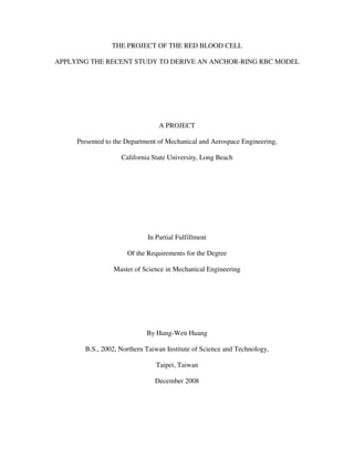
  • 26. 22 Table 2 The First result after running RK4 N ρ ( 6 10− × ) z ( 6 10− × ) 1 0.103779 0 2 0.107558 0.025393051 3 0.111336 0.04487378 : : : 994 3.859885 -0.812183029 995 3.863664 -0.845861928 996 3.867442 -0.885867513 997 3.871221 -0.938098541 998 3.875 -1.008098083230237 + 18901.44915858783i 999 3.878779 -1.008098083231395 + 37802.96842509027i 1000 3.882558 -1.008098083231395 + 37803.02086313524i Figure 8. The first result for testing the codes. z ρ
  • 27. 23 Inspection of the Result First of all, there are 7 solutions for both a and c0 in page 21. However, there are several complex numbers among these solutions (i.e. 6 complex numbers in both a and c0 as shown in page 21). Practically, These complex values may not be reasonable if one attempt to apply them in RK4. Thus, get ride of these complex solutions would be the first job before trying to solve Eq.5 and Eq.6. Since Zhou’s shape equation solution is focused on anchor-ring vesicle RBC, the frame of the result in Figure 6 shows a perfect quarter anchor-ring vesicle shape. Figure 8 shows that the first attempt did not quite hit the target. Unlike Figure 6, the last point of the curve in Figure 8 is not close enough to the ρ axis. Moreover, the result obtained from RK4 (Table2) shows complex values in the last 3 terms which are also considered impractical and negligible. Therefore, according to the inspection, it is necessary to either re-apply another set of a and c0 or reassign new values for λ , p∆ , ck , iρ , and fρ to match the best result. On the other hand, since the result obtained is a smooth and continuous curve whose tangent angle is restricted between 2 π and 2 π− , it revels that there is a high chance to achieve the goal of this project. Final Results After struggling with seeking the best values for λ , p∆ , ck , iρ , and fρ , the final solution, which could be the best results to describe the anchor-ring vesicle RBC shape, were found. The values for all parameters and constants are listed in Table 3.
  • 28. 24 Table 3 Final values for λ , p∆ , ck , ρ , a and c0 Parameter & Constant Final Value λ (Static) 2.04 6 10− × (N/m) p∆ 140 (N/m2 ) ck 7 19 10− × (NΘm) iρ 1 (Ӵm) fρ 3.875 (Ӵm) a 0.197807 2 10− × c0 -69998148.957300 By applying those values to solve Eq.5 and Eq.6 with RK4, there are 1000 points obtained to plot the results as follows: Figure 9. The quarter cross-section of the final result. ρ z
  • 29. 25 As shown in Figure 9, although the last point does not exactly on the ρ axis ( 0≠z ), the z value of the last point is –0.046337Ӵm, which is less than 4% of the peak of the curve (1.3146Ӵm), so this tiny overstepping can be tolerant. Finally, one can close up the plot by establishing a mirror image of the curve as shown in Figure 10. Figure 10. The full cross-section of the final result. Now the 3D model of the final result can be obtained by revolving the closed curve, which is shown in Figure 10, around the z axis and plotted in Figure 11, and Figure 12. ρ z
  • 30. 26 Figure 11. The full 3D model of the final result of the RBC shape equation (i.e. Eq.5 and Eq.6). ρ z y 6 10− × 6 10− × 6 10− ×
  • 31. 27 Figure 12. The cross-section of the 3D model of the RBC shape equation (i.e. Eq.5 and Eq.6). ρ z y 6 10− × 6 10− × 6 10− ×
  • 32. 28 The 3D model indicates that the final result is quite an achievement which can almost perfectly describe a shape of anchor-ring RBC, and further improvement is possible to obtain a solution for anchor-ring RBC from Zhou’s shape equation solution. With these tangible solutions, now few practical properties of Zhou’s anchor-ring vesicle RBC shape equation solution could be examined by comparing with the experimental results. They are: 1. Referring Figure 5, the outer diameter D of the final result equals =×= 875.322 fρ 7.75Ӵm, which is very compatible with the results in Figure 1 (D = 6.78 ~ 7.82Ӵm). 2. According to Mutz and Bensimon [11], the ratio between the outer diameter (D) and the width of the ring (d) in Figure 5 is 12 − . In the above final result, as shown in Figures 11 and 12 the ratio is 0.38 which represents a high agreement with Mutz and Bensimon’s experimental data. 3. The total length of the curve in Figure 9 is 4.3201Ӵm. There is no experimental data that can be compared with. However, it is able to calculate the surface area of the final model. Since the top view (y- ρ plane) is a circular shape, the surface can be calculated by applying circular area equation as follows: ( ) ( ) ][2 22 πρπρ iiclA −+×= (16) where, A is the surface area of the final model. cl is the curve length for the quarter section of the final model.
  • 33. 29 Therefore, the surface area of the final model can be calculated in the following calculation: ( ) ( ) 172]113201.4[2 22 =−+×= ππA Ӵm2 The calculation shows that the surface area of the final model is greater than the results in Figure 1. However, Due to the different shapes between biconcave-discoid and anchor-ring vesicle RBC, the inconsistent surface area is expected, but the slight difference may possibly imply that this final model could actually be a mutation shape from the standard biconcave-discoid model shown in Figure 1. Based on the above comparison, this final model shows a good agreement with these important experimental results. Although there are still some properties that are not able to confirm due to the lack of data, this final model displays a confident demonstration of the shape equation solutions proposed by Zhou for computing the shape of anchor-ring vesicle RBC. Possible Improvement in the Future Since studying in RBC is an ongoing task, more and more features, properties, and theories could be discovered. For this project, although the final model shows a good match with previous studies, there are still several possible improvements that can be studied in the future.
  • 34. 30 1. This report only applies the )(1 ρϕ (Eq.11a) as the equation to solve the primary differential equation (Eq.5), so there are still two more boundary conditions that need be tried. 2. The second equation ( )(2 ρϕ ) is run by another team member of the entire RBC project, and it represents very different results that need be examined and compared with the model in this report. 3. So far, the 3rd equation ( )(3 ρϕ ) cannot be solved because MATLAB is not able to process the high complexity of the algebraic problem. The function )(3 ρϕ represents 3 boundary conditions, which could be flexibly established a more realistic model for anchor-ring RBC. Since there is no way to obtain the solution via the aforementioned approach, looking for other algebraic or numerical method to handle the extremely complicated equation in the future is imperative. 4. Now, several properties such as diameter and surface area can be compared with the experimental data of biconcave-discoid model. Based on the limited studies so far, to better verify this analytical model proposed by Zhou, more experimental data for anchor-ring vesicle RBC are required. 5. Although Ou-Yang mentioned [2] that it is only likely to find the solutions for the specific shape one by one. Zhou’s shape equation solution may be applied to examine the general RBC shape. Figure 13 shows the cross-section and coordinate system of a biconcave-discoid model. In the figure, the angle )( iρϕ in the middle of the biconcave-discoid model is zero. Therefore, the boundary conditions listed in Eq.11a and Eq.11b have to be modified when applying Zhou’s shape equation to find a biconcave-discoid model.
  • 35. 31 Figure 13. The cross-section and coordinate system of a biconcave-discoid model. Then, the modified boundary conditions for the biconcave-discoid model can be written as follows: −= + −+−−+ ∆+ = + −+−−+ ∆+ 1 2 22 3 0 2 22 3 0 2 3 0 2 22 0 30 0 2 3 0 2 22 0 30 ff c ff c f c ii c ii c i c ca k a aca k ca k pc ca k a aca k ca k pc ρρ λ ρρ λ ρ λ ρρ λ ρρ λ ρ λ z ρ ϕ iρ fρ 0)( =iρϕ (17a) (17b)
  • 36. 32 After re-applying the three MATLAB codes with Eq.17a and Eq.17b, the examination of how compatible that Zhou’s shape equation could fit for the biconcave-discoid model has been checked as shown in the following figure. Figure 14. The full cross-section of the biconcave- discoid model which is derived from Zhou’s shape equation. As shown in Figure 14, the attempt to describe the biconcave- discoid model by applying Zhou’s shape equation solution is compared with the real experimentally recorded model shown in Figure 3c. The curve length of the quarter cross-section is 4.9446Ӵm, and iρ equals 0.05Ӵm. Therefore, by applying Eq.16, the calculated ρ z
  • 37. 33 surface area is 157Ӵm2 which is close to the models in Figure 1 (A = 135 ~ 145Ӵm2 ) than the anchor-ring model in Figures 11 and 12 (A = 172Ӵm2 ). Although the surface area is closer than what Fang and Evan’s results [3] when applying Zhou’s shape equation to obtain a similar shape with Figure 1 (the biconcave-discoid model), it is not mature to declare that Zhou’s shape equation solution is capable of dealing with biconcave- discoid model because of the insufficient experimental reference for the both biconcave-discoid and anchor-ring models. Therefore, further research of this subject is highly recommended. 6. Although the valid values of λ , p∆ , and ck were found in this study, there is no proper theory to explain how these mechanical properties could alter a RBC’s shape. Therefore, finding how tensile stress, osmotic pressure difference, and bending module would influence a RBC’s shape becomes another important research task in the future. After understanding these mechanical properties better, it is possible to establish a connection between mechanical, medical, and biophysical fields. This future study could become a precious reference to answer many human body mysteries. Summary Study the RBC’s shapes is quite a massive task. For several decades, several shape theories of RBC have been proposed by many pioneers of biophysics. By combining with several mechanical properties, to find mathematical solutions for the RBC’s shapes may contribute valuable information to help people understanding the mystery of the RBC. Although several shape equations were proposed for years, these equations were not
  • 38. 34 solved because they were presented in the form of nth order (highest order), variable coefficients, inhomogeneous and nonlinear ODE (NVIN-ODE). In a recent study, Zhou [1] proposed a new method to deal with these NVIN-ODEs and obtained a new shape equation for the anchor-ring vesicle RBC. By applying the first solution from Zhou’s shape equation solution, it shows good agreement with several experimental results. The model also suggests the possible values for tensile stress, osmotic pressure difference, and bending module.
  • 39. 35 Reference 1. Ming Zhou, Ph.D. Dissertation (2008), “Quantizing Study in Shape of Red Blood Cells,” Department of Mechanical and Aerospace Engineering, California State University, Long Beach, California 90840, USA. 2. Ou-Yang Zhong-can (1990). "Anchor ring-vesicle membranes,” Physical Review A, The American Physical Society, Vol. 41, No. 8. 3. E. Evans and Y.C. Fung (1972). “Improved Measurements of the Erychrocyte Geometry,” Microvascular Research4, P. 335-347. 4. Gov, N. and Zilman, A. G. and Safran, S (2003). “Cytoskeleton Confinement and Tension of Red Blood cell Membranes. ” Physical Review Letters, Vol. 90, No. 22, Section 228101. 5. Royalty Free Healthcare Images (2008), http://www.mediaMD.com. 6. W. Helfrich (1973). "Elastic Properties of Lipid Bilayers: Theory and Possible Experiments," Z. Naturuforsch, C28, 693. 7. Evan A. Evans (1983). "Bending Elastic Modulus of Red Blood Cell Membrane Derived From Buckling Instability in Micropipet Aspiration Tests,” Boiphys. J., Biophysical Society, Vol. 43, P27-P30. 8. M. Daoa, C.T. Limb, and S. Suresh (2003). "Mechanics of the human red blood cell deformed by optical tweezers,” Journal of the Mechanics and Physics of Solids, Vol. 51, P2259-P2280. 9. Ou-Yang Zhong-can and W. Helfrich (1987). "Instability and Deformation of a Spherical Vesicle by Pressure,” Physical Review letters, Vol. 59, No. 21, P2486-P2488. 10. E. W. Hobson (1955), “The Theory of Spherical and Ellipsoidal Harmonics,” Cambridge, Cambridge, England.
  • 40. 36 11. M. Mutz and D. Bensimon (1991). "Observation of toroidal vesicles,” Physical Review A, The American Physical Society, Vol. 43, No. 8. 12. J. G. Hu and Z. C. Ou-Yang (1993), “Shape Equations of the Axisymmetric Vesicles,” Phys. Rev, E47, p462, 1993. 13. Ming Zhou and H.Y. Yeh (2008), “Red Blood Cell Project Guide for Spring 2008,” Department of Mechanical and Aerospace Engineering, California State University, Long Beach, California 90840, USA. 14. Ramin S. Esfandiari (2007), “Applied Mathematics for Engineers,” Fourth Edition, ATLANTIS PUBLISHING COMPANY, P.945-P.958.
  • 41. 37 Appendix A c0a.m function [ar, cra] = c0a(coeffs) %Find c0 and a % % [a, c0] = c0a([L k p r z]) where % % L is lamda. % k is kc. % p is delta p. % r is rowf. % z is rowi. % % ar is the result of a. % cra is the result of c0. % % Example: % [a, c0] = c0a([4e-6 4.35e-19 102.5 3.875e-6 1e-7]) if nargin ~= 1 || size(coeffs,2) ~= 5 L = 4e-6; %Lamda, the middle value in the range. k = 4.35e-19; %kc, middle value in the range p = 102.5; %Delta p, the middle value in the range r = 3.875e-6; %Rowf, the middle value in the range z = 1e-7 %Rowi, which is very close to zero else L = coeffs(1,1); k = coeffs(1,2); p = coeffs(1,3); r = coeffs(1,4); z = coeffs(1,5); end syms c a %symbolized c0 and a A = ((L*c+p)/k)*z^3; B = a*(c^2-(L/k))*z^2; C = ((3*(a^2)*c)/2) * z; D = ((a^3)/2)-a; E = ((2*L)/k)*z^2; F = a*c*z; f1sac = strcat(char(A+B-C+D-E-F), '=0'); f1 = (A+B-C+D)/(E+F); A = ((L*c+p)/k)*r^3; B = a*(c^2-(L/k))*r^2; C = ((3*(a^2)*c)/2) * r; D = ((a^3)/2)-a; E = ((2*L)/k)*r^2; F = a*c*r; f2sac = strcat(char(A+B-C+D+E+F), '=0'); f2 = (A+B-C+D)/(E+F); [ar,cra] = solve(f1sac,f2sac,'a,c');
  • 42. 38 Appendix B RK4Method.m function [x, y] = RK4Method(x0, N, h, f, y0) %RK4 Method %given in the form y' = f(x, y). % % [x, y] = RK4Method(x0, N, h, f, y0) where % % x0 is a scalar representing the initial value of x. % N is number of nodes. % h is the distance between each node. % f is an inline function representing y' = f(x, y). % y0 is the initial condition of y. % % x is the vector to store each value of x in each node. % y is the vector to store each value of y in each node. q1 = 0; q2 = 0; q3 = 0; q4 = 0; x = zeros(N,1); y = zeros(N,1); x(1) = x0; y(1) = y0; for n = 1:N q1 = h * f(x(n), y(n)); q2 = h * f(x(n) + (h / 2), y(n) + (q1 / 2)); q3 = h * f(x(n) + (h / 2), y(n) + (q2 / 2)); q4 = h * f(x(n) + h, y(n) + q3); y(n+1) = y(n) + ((q1 + 2 * q2 + 2 * q3 + q4) / 6); x(n+1) = x(n) + h; end
  • 43. 39 Appendix C c0a_RK4.m function [f, ar, cra, row, z] = c0a_RK4(coeffs, range) % Run RK4 from c0-a % % [f, a, c0] = c0a_RK4([L k p], [rowi rowf n]) where % % L is lamda. % k is kc. % p is delta p. % r is rowf. % z is rowi. % n is numbers of the running steps for RK4. % % f is the differential equation z'. % ar is the result of a. % cra is the result of c0. % % Example: % [f, a, c0, row, z] = c0a_RK4([4e-6 4.35e-19 102.5], [1e-7 3.875e-6 1000]) % [f, a, c0, row ,z] = c0a_RK4([L k p], [rowi rowf n]) L = coeffs(1,1); %Lamda k = coeffs(1,2); %kc p = coeffs(1,3); %Delta p rowi = range(1,1); rowf = range(1,2); [ar, cra] = c0a([L k p rowf rowi]); %solve c0 and a syms r z; % Symbolize row and z a = ar (1,1); %a c = cra(1,1); %c0 L = coeffs(1,1); %Lamda k = coeffs(1,2); %kc p = coeffs(1,3); %Delta p A = ((L*c+p)/k)*r^3; B = a*(c^2-(L/k))*r^2; C = ((3*(a^2)*c)/2) * r; D = ((a^3)/2)-a; E = ((2*L)/k)*r^2; F = a*c*r; f = vectorize(inline(char(tan(asin((A+B-C+D)/(E+F)))),'r','z')); N = range(1,3)-2; h = (range(1,2) - range(1,1))/(range(1,3)); row0 = range(1,1) + h; z0 = 0; [row, z] = RK4Method(row0, N, h, f, z0); plot(row,z),grid,hold;