A hand-waving introduction to sparsity for compressed tomography reconstruction
•
3 likes•2,391 views

The document provides a hand-waving introduction to using sparsity for compressed tomography reconstruction. It discusses how imposing sparsity can help solve ill-posed inverse problems with limited data by finding sparse solutions. Mathematical formulations are presented using L1-norm minimization and techniques like total variation. Optimization algorithms like iterative shrinkage-thresholding are described, which use proximal operators to handle non-smooth terms in the objective function.

Recommended
Recommended
More Related Content
What's hot
What's hot (19)
Similar to A hand-waving introduction to sparsity for compressed tomography reconstruction
Similar to A hand-waving introduction to sparsity for compressed tomography reconstruction (20)
More from Gael Varoquaux
More from Gael Varoquaux (20)
Recently uploaded
Recently uploaded (20)
A hand-waving introduction to sparsity for compressed tomography reconstruction
- 1. A hand-waving introduction to sparsity for compressed tomography reconstruction Ga¨l Varoquaux and Emmanuelle Gouillart e Dense slides. For future reference: http://www.slideshare.net/GaelVaroquaux
- 2. 1 Sparsity for inverse problems 2 Mathematical formulation 3 Choice of a sparse representation 4 Optimization algorithms G Varoquaux 2
- 3. 1 Sparsity for inverse problems Problem setting Intuitions G Varoquaux 3
- 4. 1 Tomography reconstruction: a linear problem y = Ax 0 20 40 60 80 0 50 100 150 200 250 y ∈ Rn, A ∈ Rn×p, x ∈ Rp n ∝ number of projections p: number of pixels in reconstructed image We want to find x knowing A and y G Varoquaux 4
- 5. 1 Small n: an ill-posed linear problem y = Ax admits multiple solutions The sensing operator A has a large null space: images that give null projections In particular it is blind to high spatial frequencies: G Varoquaux 5
- 6. 1 Small n: an ill-posed linear problem y = Ax admits multiple solutions The sensing operator A has a large null space: images that give null projections In particular it is blind to high spatial frequencies: Large number of projections Ill-conditioned problem: “short-sighted” rather than blind, ⇒ captures noise on those components G Varoquaux 5
- 7. 1 A toy example: spectral analysis Recovering the frequency spectrum Signal Freq. spectrum signal = A · frequencies 0 2 4 6 8 ... 0 10 20 30 40 50 60 G Varoquaux 6
- 8. 1 A toy example: spectral analysis Sub-sampling Signal Freq. spectrum signal = A · frequencies 0 2 4 6 8 ... 0 10 20 30 40 50 60 Recovery problem becomes ill-posed G Varoquaux 6
- 9. 1 A toy example: spectral analysis Problem: aliasing Signal Freq. spectrum Information in the null-space of A is lost G Varoquaux 7
- 10. 1 A toy example: spectral analysis Problem: aliasing Signal Freq. spectrum Solution: incoherent measurements Signal Freq. spectrum i.e. careful choice of null-space of A G Varoquaux 7
- 11. 1 A toy example: spectral analysis Incoherent measurements, but scarcity of data Signal Freq. spectrum The null-space of A is spread out in frequency Not much data ⇒ large null-space = captures “noise” G Varoquaux 8
- 12. 1 A toy example: spectral analysis Incoherent measurements, but scarcity of data Signal Freq. spectrum The null-space of A is spread out in frequency Not much data ⇒ large null-space Sparse Freq. spectrum = captures “noise” Impose sparsity Find a small number of frequencies to explain the signal G Varoquaux 8
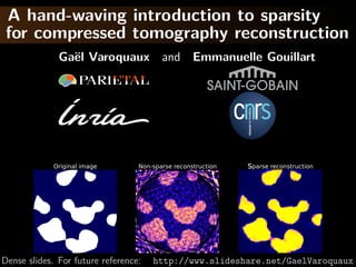
- 13. 1 And for tomography reconstruction? Original image Non-sparse reconstruction Sparse reconstruction 128 × 128 pixels, 18 projections http://scikit-learn.org/stable/auto_examples/applications/ plot_tomography_l1_reconstruction.html G Varoquaux 9
- 14. 1 Why does it work: a geometric explanation Two coefficients of x not in the null-space of A: x2 y= Ax xtrue x1 The sparsest solution is in the blue cross It corresponds to the true solution (xtrue ) if the slope is > 45◦ G Varoquaux 10
- 15. 1 Why does it work: a geometric explanation Two coefficients of x not in the null-space of A: x2 y= Ax xtrue x1 The sparsest solution is in the blue cross It corresponds to the true solution (xtrue ) if the slope is > 45◦ The cross can be replaced by its convex hull G Varoquaux 10
- 16. 1 Why does it work: a geometric explanation Two coefficients of x not in the null-space of A: x2 y= Ax xtrue x1 The sparsest solution is in the blue cross It corresponds to the true solution (xtrue ) if the slope is > 45◦ In high dimension: large acceptable set G Varoquaux 10
- 17. Recovery of sparse signal Null space of sensing operator incoherent with sparse representation ⇒ Excellent sparse recovery with little projections Minimum number of observations necessary: nmin ∼ k log p, with k: number of non zeros [Candes 2006] Rmk Theory for i.i.d. samples Related to “compressive sensing” G Varoquaux 11
- 18. 2 Mathematical formulation Variational formulation Introduction of noise G Varoquaux 12
- 19. 2 Maximizing the sparsity 0 number of non-zeros min 0(x) x s.t. y = A x x2 y= Ax xtrue x1 “Matching pursuit” problem [Mallat, Zhang 1993] “Orthogonal matching pursuit” [Pati, et al 1993] Problem: Non-convex optimization G Varoquaux 13
- 20. 2 Maximizing the sparsity 1 (x) = i |xi | min 1(x) x s.t. y = A x x2 y= Ax xtrue x1 “Basis pursuit” [Chen, Donoho, Saunders 1998] G Varoquaux 13
- 21. 2 Modeling observation noise y = Ax + e e = observation noise New formulation: 2 min 1 (x) x s.t. y = A x y − Ax 2 ≤ ε2 Equivalent: “Lasso estimator” [Tibshirani 1996] 2 min y − Ax x 2 + λ 1(x) G Varoquaux 14
- 22. 2 Modeling observation noise y = Ax + e e = observation noise New formulation: 2 min 1 (x) x s.t. y = A x y − Ax 2 ≤ ε2 Equivalent: “Lasso estimator” [Tibshirani 1996] 2 x2 min y − Ax x 2 + λ 1(x) Data fit Penalization x1 Rmk: kink in the 1 ball creates sparsity G Varoquaux 14
- 23. 2 Probabilistic modeling: Bayesian interpretation P(x|y) ∝ P(y|x) P(x) ( ) “Posterior” Forward model “Prior” Quantity of interest Expectations on x Forward model: y = A x + e, e: Gaussian noise ⇒ P(y|x) ∝ exp − 2 1 2 y − A x 2 σ 2 1 Prior: Laplacian P(x) ∝ exp − µ x 1 1 2 1 Negated log of ( ): 2σ 2 y − Ax 2 + µ 1 (x) Maximum of posterior is Lasso estimate Note that this picture is limited and the Lasso is not a good G Varoquaux Bayesian estimator for the Laplace prior [Gribonval 2011]. 15
- 24. 3 Choice of a sparse representation Sparse in wavelet domain Total variation G Varoquaux 16
- 25. 3 Sparsity in wavelet representation Typical images Haar decomposition Level 1 Level 2 Level 3 are not sparse Level 4 Level 5 Level 6 ⇒ Impose sparsity in Haar representation A → A H where H is the Haar transform G Varoquaux 17
- 26. 3 Sparsity in wavelet representation Original image Non-sparse reconstruction Typical images Haar decomposition Level 1 Level 2 Level 3 are not sparse Level 4 Level 5 Level 6 Sparse image Sparse in Haar ⇒ Impose sparsity in Haar representation A → A H where H is the Haar transform G Varoquaux 17
- 27. 3 Total variation Impose a sparse gradient 2 min y − Ax x 2 +λ ( x)i 2 i 12 norm: 1 norm of the gradient magnitude Sets x and y to zero jointly Original image Haar wavelet TV penalization G Varoquaux 18
- 28. 3 Total variation Impose a sparse gradient 2 min y − Ax x 2 +λ ( x)i 2 i 12 norm: 1 norm of the gradient magnitude Sets x and y to zero jointly Original image Error for Haar wavelet Error for TV penalization G Varoquaux 18
- 29. 3 Total variation + interval Bound x in [0, 1] 2 min y−Ax x 2+λ ( x)i 2 +I([0, 1]) i Original image TV penalization TV + interval G Varoquaux 19
- 30. 3 Total variation + interval Bound x in [0, 1] 2 min y−Ax x 2+λ ( x)i 2 +I([0, 1]) i TV Rmk: Constraint Histograms: TV + interval does more than fold- ing values outside of the range back in. 0.0 0.5 1.0 Original image TV penalization TV + interval G Varoquaux 19
- 31. 3 Total variation + interval Bound x in [0, 1] 2 min y−Ax x 2+λ ( x)i 2 +I([0, 1]) i TV Rmk: Constraint Histograms: TV + interval does more than fold- ing values outside of the range back in. 0.0 0.5 1.0 Original image Error for TV penalization Error for TV + interval G Varoquaux 19
- 32. Analysis vs synthesis 2 Wavelet basis min y − A H x 2 + x 1 H Wavelet transform Total variation min y − A x 2 + Dx 2 1 D Spatial derivation operator ( ) G Varoquaux 20
- 33. Analysis vs synthesis Wavelet basis min y − A H x 2 + x 2 1 H Wavelet transform “synthesis” formulation Total variation min y − A x 2 + Dx 2 1 D Spatial derivation operator ( ) “analysis” formulation Theory and algorithms easier for synthesis Equivalence iif D is invertible G Varoquaux 20
- 34. 4 Optimization algorithms Non-smooth optimization ⇒ “proximal operators” G Varoquaux 21
- 35. 4 Smooth optimization fails! Gradient descent Gradient descent x2 Energy Iterations x1 Smooth optimization fails in non-smooth regions These are specifically the spots that interest us G Varoquaux 22
- 36. 4 Iterative Shrinkage-Thresholding Algorithm Settings: min f + g; f smooth, g non-smooth f and g convex, f L-Lipschitz Typically f is the data fit term, and g the penalty 1 2 1 ex: Lasso 2σ 2 y − Ax 2 + µ 1 (x) G Varoquaux 23
- 37. 4 Iterative Shrinkage-Thresholding Algorithm Settings: min f + g; f smooth, g non-smooth f and g convex, f L-Lipschitz Minimize successively: (quadratic approx of f ) + g f (x) < f (y) + x − y, f (y) 2 +L x − y 2 2 Proof: by convexity f (y) ≤ f (x) + f (y) (y − x) in the second term: f (y) → f (x) + ( f (y) − f (x)) upper bound last term with Lipschitz continuity of f L 1 2 xk+1 = argmin g(x) + x − xk − f (xk ) 2 x 2 L [Daubechies 2004] G Varoquaux 23
- 38. 4 Iterative Shrinkage-Thresholding Algorithm Step 1: Gradient descentsmooth, g non-smooth Settings: min f + g; f on f f and g convex, f L-Lipschitz Step 2: Proximal operator of g: Minimize proxλg (x) def argmin y − x 2 + λ g(y) successively: = 2 y (quadratic approx of f ) + g Generalization of Euclidean projection f (x) < f (y) + x − y, f (y)1} on convex set {x, g(x) ≤ 2 Rmk: if g is the indicator function +L x − y 2 2 of a set S, the proximal operator is the Euclidean projection. Proof: by convexity f (y) ≤ f (x) + f (y) (y − x) prox in theλ 1 (x) = sign(x ) x − λ second term: f (y) → f (x) + ( i f (y) − f (x)) i + upper bound last term with Lipschitz continuity of f “soft thresholding” L 1 2 xk+1 = argmin g(x) + x − xk − f (xk ) 2 x 2 L [Daubechies 2004] G Varoquaux 23
- 39. 4 Iterative Shrinkage-Thresholding Algorithm Gradient descent x2 ISTA Energy Iterations x1 Gradient descent step G Varoquaux 24
- 40. 4 Iterative Shrinkage-Thresholding Algorithm Gradient descent x2 ISTA Energy Iterations x1 Projection on 1 ball G Varoquaux 24
- 41. 4 Iterative Shrinkage-Thresholding Algorithm Gradient descent x2 ISTA Energy Iterations x1 Gradient descent step G Varoquaux 24
- 42. 4 Iterative Shrinkage-Thresholding Algorithm Gradient descent x2 ISTA Energy Iterations x1 Projection on 1 ball G Varoquaux 24
- 43. 4 Iterative Shrinkage-Thresholding Algorithm Gradient descent x2 ISTA Energy Iterations x1 Gradient descent step G Varoquaux 24
- 44. 4 Iterative Shrinkage-Thresholding Algorithm Gradient descent x2 ISTA Energy Iterations x1 Projection on 1 ball G Varoquaux 24
- 45. 4 Iterative Shrinkage-Thresholding Algorithm Gradient descent x2 ISTA Energy Iterations x1 Gradient descent step G Varoquaux 24
- 46. 4 Iterative Shrinkage-Thresholding Algorithm Gradient descent x2 ISTA Energy Iterations x1 Projection on 1 ball G Varoquaux 24
- 47. 4 Iterative Shrinkage-Thresholding Algorithm Gradient descent x2 ISTA Energy Iterations x1 G Varoquaux 24
- 48. 4 Fast Iterative Shrinkage-Thresholding Algorithm FISTA Gradient descent x2 ISTA FISTA Energy Iterations x1 As with conjugate gradient: add a memory term ISTA tk −1 dxk+1 = dxk+1 + tk+1 (dxk − dxk−1 ) √ 1+ 2 1+4 tk t1 = 1, tk+1 = 2 ⇒ O(k −2 ) convergence [Beck Teboulle 2009] G Varoquaux 25
- 49. 4 Proximal operator for total variation Reformulate to smooth + non-smooth with a simple projection step and use FISTA: [Chambolle 2004] 2 proxλTV x = argmin y − x 2 +λ ( x)i 2 x i G Varoquaux 26
- 50. 4 Proximal operator for total variation Reformulate to smooth + non-smooth with a simple projection step and use FISTA: [Chambolle 2004] 2 proxλTV x = argmin y − x 2 +λ ( x)i 2 x i 2 = argmax λ div z + y 2 z, z ∞ ≤1 Proof: “dual norm”: v 1 = max v, z z ∞ ≤1 div is the adjoint of : v, z = v, −div z Swap min and max and solve for x Duality: [Boyd 2004] This proof: [Michel 2011] G Varoquaux 26
- 51. Sparsity for compressed tomography reconstruction @GaelVaroquaux 27
- 52. Sparsity for compressed tomography reconstruction Add penalizations with kinks x2 Choice of prior/sparse representation Non-smooth optimization (FISTA) x1 Further discussion: choice of prior/parameters Minimize reconstruction error from degraded data of gold-standard acquisitions Cross-validation: leave half of the projections and minimize projection error of reconstruction Python code available: https://github.com/emmanuelle/tomo-tv @GaelVaroquaux 27
- 53. Bibliography (1/3) [Candes 2006] E. Cand`s, J. Romberg and T. Tao, Robust uncertainty e principles: Exact signal reconstruction from highly incomplete frequency information, Trans Inf Theory, (52) 2006 [Wainwright 2009] M. Wainwright, Sharp Thresholds for High-Dimensional and Noisy Sparsity Recovery Using 1 constrained quadratic programming (Lasso), Trans Inf Theory, (55) 2009 [Mallat, Zhang 1993] S. Mallat and Z. Zhang, Matching pursuits with Time-Frequency dictionaries, Trans Sign Proc (41) 1993 [Pati, et al 1993] Y. Pati, R. Rezaiifar, P. Krishnaprasad, Orthogonal matching pursuit: Recursive function approximation with plications to wavelet decomposition, 27th Signals, Systems and Computers Conf 1993 @GaelVaroquaux 28
- 54. Bibliography (2/3) [Chen, Donoho, Saunders 1998] S. Chen, D. Donoho, M. Saunders, Atomic decomposition by basis pursuit, SIAM J Sci Computing (20) 1998 [Tibshirani 1996] R. Tibshirani, Regression shrinkage and selection via the lasso, J Roy Stat Soc B, 1996 [Gribonval 2011] R. Gribonval, Should penalized least squares regression be interpreted as Maximum A Posteriori estimation?, Trans Sig Proc, (59) 2011 [Daubechies 2004] I. Daubechies, M. Defrise, C. De Mol, An iterative thresholding algorithm for linear inverse problems with a sparsity constraint, Comm Pure Appl Math, (57) 2004 @GaelVaroquaux 29
- 55. Bibliography (2/3) [Beck Teboulle 2009], A. Beck and M. Teboulle, A fast iterative shrinkage-thresholding algorithm for linear inverse problems, SIAM J Imaging Sciences, (2) 2009 [Chambolle 2004], A. Chambolle, An algorithm for total variation minimization and applications, J Math imag vision, (20) 2004 [Boyd 2004], S. Boyd and L. Vandenberghe, Convex Optimization, Cambridge University Press 2004 — Reference on convex optimization and duality [Michel 2011], V. Michel et al., Total variation regularization for fMRI-based prediction of behaviour, Trans Med Imag (30) 2011 — Proof of TV reformulation: appendix C @GaelVaroquaux 30