Isotope hydrogeochemistry of Bangui Urban-Zone GW
•Download as DOC, PDF•
1 like•601 views

First paper of isotope hydrology and geochemistry of Bangui, Central Africa
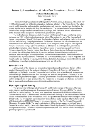
![Decimal coordinates of wells, Bangui, (large deep red-colored spots = high ionic charge)
1o '
1o '
1o '
1o '
1o '
1o '
1o '
1o '
1o '
1o '
83
7
82
8
82
9
83
0
83
1
83
2
83
83
4
83
5
83
6
4.46 AIRPORT
13 - PK12 longi 18° 27'
4.45 (Ecole Begoua) 4 o 27'
longi 18° 28'
longi 18° 29'
4.44
longi 18° 30'
4 o 26'
4.43 longi 18° 31'
longi 18° 32'
4.42 12 - PK10 4 o 25' longi 18° 33'
4.41 longi 18° 34'
longi 18° 35'
4.40 4 o 24' longi 18° 36'
10 - Boy Rabe
longi 18° 37'
4.39
Latitude longi 18° 38'
4 o 23'
4.38 lati 4° 19'
2 - Gbangouma lati 4° 20'
4.37 11 - Boy Rabe
lati 4° 21'
(Kaimba)
4 - Ngarangba 3 - Ouango lati 4° 22'
4.36 (nogopou) lati 4° 23'
1 - UNICEF
4.35 4 o 21' lati 4° 24'
5-Ecole lati 4° 25'
4.34 8 - Guitangola St. Jean
lati 4° 26'
(F)
4 o 20'
lati 4° 27'
4.33 9 - Guitangola
7 - Bimbo
(Soeurs) well location
(Puit)
4.32 6 - Bimbo NO3-
4 o 19'
(Usaca) 2km distance
4.31
8 5
1 .4
8 6
1 .4
8 7
1 .4
8 8
1 .4
8 9
1 .4
8 0
1 .5
8 1
1 .5
8 2
1 .5
8 3
1 .5
8 4
1 .5
8 5
1 .5
8 6
1 .5
8 7
1 .5
8 8
1 .5
8 9
1 .5
8 0
1 .6
8 1
1 .6
8 2
1 .6
8 3
1 .6
8 4
1 .6
Longitude
Figure 1 Sample well field. Red spots show the ionic-charge. Black squares show NO3--polluted sites
Methods and Results
1. Sampling and Analysis
Groundwater samples were collected in April 2007 from thirteen pumping-wells drilled in the
semi-confined aquifer, seven heavy-storm events as well as one run-off aliquot and one Oubangui
River-water were sampled mostly during dry-season of the year 2007 (Table 1 and Figure 1). The
samples were shipped for chemical and stable-isotope analysis (18O and 2H) at the Atomic Energy
Authority, Cairo, Egypt, using the standard methods. The isotopic composition was measured on
mass-spectrometer after CO2 equilibrium with water or after water reduction on hot zinc for δ18O
and δ2H, respectively.
2. Hydrogeochemical data
The hydrochemical and isotope data is plotted in several ways (Figures 2 to 12). Groundwater
temperature is high (24 to 28.6°C) and enhances water reaction with aquifer solid-phases. It seems
that a karstic porosity allows rapid circulation showing initial high temperature of ~28°C with low
EC of 50 µmoh/cm, whereas in the deep porous sections the EC is variable, up to 600 µmoh/cm
(relatively high EC where recharge warm water, T>24°C, is circulating.)
The pH is the masterpiece of hydrochemical reactions. The local air-born dust is made-up of
fine reddish oxide- and silicate-particles [e.g. Gibbsite, Al2O3.3H2O, Goethite, α−FeOOH and
Kaolinite, Al2Si2O5(OH)4]. Reaction of rainwater with such dust may result in significantly
increasing its pH value before reaching the ground. The pH of any rainwater might become as high
as 8.26 when it becomes saturated in air-born Calcite-dust during rainfall (Harte, 1985, page 108.)
________________________________________________________________________________________________
Isotope Hydrochemistry of Urban Zone Groundwater, Central Africa. (Mohamed Fahmy Hussein) 2](data:image/gif;base64,R0lGODlhAQABAIAAAAAAAP///yH5BAEAAAAALAAAAAABAAEAAAIBRAA7)
Recommended
More Related Content
Recently uploaded
Recently uploaded (20)
Featured
Featured (20)
Isotope hydrogeochemistry of Bangui Urban-Zone GW
- 1. Isotope Hydrogeochemistry of Urban-Zone Groundwater, Central Africa Mohamed Fahmy Hussein Cairo University, Egypt Abstract The isotope hydrogeochemistry of Bangui City, Central Africa, is discussed. This small city (~0.65 million people on ~20km2) is situated on Oubangui tributary of the Congo River. The urban- zone is highly despoiled and most of its population depends on water supply from the shallow the porous aquifer and/or pumping the deep fractured aquifer. The purpose is to define groundwater chemical and isotope composition in relation to recharge, rock formation and the impact of the awful practices of the indigenous population on groundwater quality. The hydrochemical data demonstrated reaction with biogenic CO2 gas, weathering, cation- exchange and NO3- pollution of anthropogenic origin. The conjunctive use of the chemical and isotope compositions (18O and 2H) showed the alteration of silicate and carbonate rocks in the zones of dilute and relatively charged groundwater. The isotopes illustrated the role of evaporation and transpiration in the water-balance, with a fraction of the transpired-vapor recycled. The regional “inverse continental isotope-effect” is attributed to differences in air-temperature, amount and altitude of precipitation, rather than to a claimed movement of humid air masses from Central Africa westward to the Atlantic. Isotope data showed that recharge during the humid-season may not exceed that taking place during the dry-season, and that the overall aquifer-recharge is mediocre. The data helped to distinguish rapid circulation in deep fractured formations northward versus slow one in porous sections southward, and showed that the system is void of evaporites and its carbonates are made-up of Calcite, not Dolomite. Pollution, by nitrate, is noticed downtown, and would extend everywhere in that urban-zone due to its law life-style. Introduction Africa, south of the Sahara, has abundant surface and groundwater basins that are seldom studied. Oubangui River is the northern tributary of Congo River. It flows in a SW direction, making part of the border between Congo and Central African Rep., where Bangui, is constructed one century ago. Despite abundant river discharge and plentiful precipitation (1500mm.yr-1), the city depends on groundwater supply. This study gives the first account on the hydrochemical and isotope compositions of local groundwater. The objective is to conjugate geochemical and isotope data to understand groundwater composition and aquifer dynamics. Hydrogeological Setting The groundwater of Bangui city (Figures 1A and B) is the subject of this study. The local water-balance, aquifer recharge and dynamics are not well-known (Doyemet, 2006). The city is underlain by two formations. The upper is an unconfined porous aquifer (100mdeep Quaternary Oxisols) and the lower (~200m thick) is a semi-confined one made-up of fractured carbonate and/or silicate rocks (underlain by the Precambrian schist and quartzite basement) where we sampled some drilled wells. The two aquifers are hydraulically connected via a clay aquitard. The fractures run in a SE direction formed 550±100 Ma ago by orogenesis tectonics of the Pan-African Oubanguide Mountains (Kennedy, 1964). The local precipitation is falling in two seasons; wet (April/May to October/November) and dry (November/December to March/April) and 85% of rainfall takes place during the wet-season. The annual mean air-temperature exceeds 26°C and the relative humidity is generally high (>0.85) year-round. ________________________________________________________________________________________________ Isotope Hydrochemistry of Urban Zone Groundwater, Central Africa. (Mohamed Fahmy Hussein) 1
- 2. Decimal coordinates of wells, Bangui, (large deep red-colored spots = high ionic charge) 1o ' 1o ' 1o ' 1o ' 1o ' 1o ' 1o ' 1o ' 1o ' 1o ' 83 7 82 8 82 9 83 0 83 1 83 2 83 83 4 83 5 83 6 4.46 AIRPORT 13 - PK12 longi 18° 27' 4.45 (Ecole Begoua) 4 o 27' longi 18° 28' longi 18° 29' 4.44 longi 18° 30' 4 o 26' 4.43 longi 18° 31' longi 18° 32' 4.42 12 - PK10 4 o 25' longi 18° 33' 4.41 longi 18° 34' longi 18° 35' 4.40 4 o 24' longi 18° 36' 10 - Boy Rabe longi 18° 37' 4.39 Latitude longi 18° 38' 4 o 23' 4.38 lati 4° 19' 2 - Gbangouma lati 4° 20' 4.37 11 - Boy Rabe lati 4° 21' (Kaimba) 4 - Ngarangba 3 - Ouango lati 4° 22' 4.36 (nogopou) lati 4° 23' 1 - UNICEF 4.35 4 o 21' lati 4° 24' 5-Ecole lati 4° 25' 4.34 8 - Guitangola St. Jean lati 4° 26' (F) 4 o 20' lati 4° 27' 4.33 9 - Guitangola 7 - Bimbo (Soeurs) well location (Puit) 4.32 6 - Bimbo NO3- 4 o 19' (Usaca) 2km distance 4.31 8 5 1 .4 8 6 1 .4 8 7 1 .4 8 8 1 .4 8 9 1 .4 8 0 1 .5 8 1 1 .5 8 2 1 .5 8 3 1 .5 8 4 1 .5 8 5 1 .5 8 6 1 .5 8 7 1 .5 8 8 1 .5 8 9 1 .5 8 0 1 .6 8 1 1 .6 8 2 1 .6 8 3 1 .6 8 4 1 .6 Longitude Figure 1 Sample well field. Red spots show the ionic-charge. Black squares show NO3--polluted sites Methods and Results 1. Sampling and Analysis Groundwater samples were collected in April 2007 from thirteen pumping-wells drilled in the semi-confined aquifer, seven heavy-storm events as well as one run-off aliquot and one Oubangui River-water were sampled mostly during dry-season of the year 2007 (Table 1 and Figure 1). The samples were shipped for chemical and stable-isotope analysis (18O and 2H) at the Atomic Energy Authority, Cairo, Egypt, using the standard methods. The isotopic composition was measured on mass-spectrometer after CO2 equilibrium with water or after water reduction on hot zinc for δ18O and δ2H, respectively. 2. Hydrogeochemical data The hydrochemical and isotope data is plotted in several ways (Figures 2 to 12). Groundwater temperature is high (24 to 28.6°C) and enhances water reaction with aquifer solid-phases. It seems that a karstic porosity allows rapid circulation showing initial high temperature of ~28°C with low EC of 50 µmoh/cm, whereas in the deep porous sections the EC is variable, up to 600 µmoh/cm (relatively high EC where recharge warm water, T>24°C, is circulating.) The pH is the masterpiece of hydrochemical reactions. The local air-born dust is made-up of fine reddish oxide- and silicate-particles [e.g. Gibbsite, Al2O3.3H2O, Goethite, α−FeOOH and Kaolinite, Al2Si2O5(OH)4]. Reaction of rainwater with such dust may result in significantly increasing its pH value before reaching the ground. The pH of any rainwater might become as high as 8.26 when it becomes saturated in air-born Calcite-dust during rainfall (Harte, 1985, page 108.) ________________________________________________________________________________________________ Isotope Hydrochemistry of Urban Zone Groundwater, Central Africa. (Mohamed Fahmy Hussein) 2
- 3. Table 1 Hydrochemical and isotope data Sample date Site T °C pH pH EC dis.O 2 Ca 2+ Mg 2+ Na + + K HCO3 Cl - - SO4 2- NO3 - δ 18O δ 2H + Σ +Σ - -1 -1 no. field lab µ S.cm -1 mg.l -1 meq.l /SMOW% o meq l 11 28-Apr-2007 Boy Rabe (Kaimba) 26.6 5.11 8.07 19.5 2.53 0.03 0.01 0.12 0.03 0.09 0.05 0.02 0.03 -2.21 -7.75 0.35 B a n g u i C i t y , R C A, C e n t r a l A f r i c a 9 28-Apr-2007 Guitangola 24.0 6.87 7.95 19.5 0.80 0.09 0.04 0.19 0.02 0.14 0.11 0.02 0.07 -1.74 -4.28 0.61 10 28-Apr-2007 Boy Rabe 26.7 5.45 7.90 59.6 2.40 0.10 0.04 0.30 0.08 0.07 0.15 0.03 0.26 -2.03 -3.32 0.76 3 28-Apr-2007 O uango (Nogopou) 27.7 5.77 7.70 59.0 2.31 0.23 0.21 0.25 0.02 0.64 0.05 0.05 0.003 -2.44 -8.62 1.45 2 28-Apr-2007 Gbangouma 28.6 5.63 7.68 64.5 2.20 0.24 0.18 0.33 0.02 0.68 0.06 0.05 0.02 -2.17 -3.38 1.56 4 28-Apr-2007 Ngarangba 28.2 5.32 7.61 183.0 3.40 0.37 0.38 0.46 0.13 0.49 0.73 0.09 0.65 -1.92 -2.53 2.22 1 28-Apr-2007 UNIC EF 28.0 5.91 7.51 228.0 1.00 0.86 0.36 0.45 0.03 1.10 0.28 0.14 0.34 -0.67 5.59 3.21 12 28-Apr-2007 PK 10 25.0 6.34 7.46 290.0 1.88 1.31 0.62 0.78 0.04 2.81 0.07 0.02 0.005 -2.00 -4.50 5.65 8 28-Apr-2007 Guitangol (F) 25.7 6.18 7.41 332.0 3.40 3.16 0.06 0.11 0.02 3.45 0.08 0.10 0.03 -1.91 -1.52 6.99 13 28-Apr-2007 PK12 (Ecole Begoua) 26.3 6.28 7.46 283.0 2.10 2.30 0.80 0.77 0.02 2.94 0.13 0.03 0.02 -2.31 -5.70 6.99 7 28-Apr-2007 Bimbo (Soeurs) 25.1 6.45 7.38 522.0 1.83 2.99 2.10 0.23 0.03 5.76 0.04 0.06 0.01 -2.13 -6.27 11.20 5 28-Apr-2007 Ecole St. Jean (Lakouanga) 25.6 6.90 7.63 516.0 3.61 3.10 2.37 0.18 0.02 5.81 0.14 0.05 0.02 -2.13 -4.75 11.68 6 28-Apr-2007 Bimbo (Usaca) 26.0 6.72 7.43 644.0 2.57 4.18 1.99 0.20 0.02 6.27 0.64 0.06 0.004 -1.91 -5.25 13.36 19 26-Mar-2007 Rain wate r 7.61 26.0 0.31 0.01 0.11 0.03 0.28 0.04 0.09 0.004 1.92 28.25 0.87 20 26-Mar-2007 "" 6.46 30.0 0.37 0.01 0.06 0.03 0.38 0.03 0.02 0.003 0.91 18 23-Mar-2007 "" 7.81 38.0 0.36 0.02 0.23 0.03 0.43 0.05 0.06 0.03 -0.23 19.54 1.19 15 18-Feb-2007 "" 7.34 86.0 0.62 0.08 0.22 0.08 0.62 0.12 0.18 0.0002 1.92 16 20-Feb-2007 " " (e vaporate d ?) 7.71 114.0 0.35 0.07 0.49 0.16 0.84 0.10 0.05 0.01 7.96 45.15 2.06 17 19-Mar-2007 "" 7.70 75.0 0.61 0.07 0.27 0.13 0.79 0.11 0.12 0.02 0.86 22.25 2.09 14 28-Jan-2007 "" 6.01 119.0 0.36 0.08 0.46 0.21 0.78 0.33 0.09 0.02 2.91 30.89 2.31 run off 28-Apr-2007 Run-off wate r, at Boy-Rab -5.46 -39.54 21 1-Apr-2007 Rive r O ubangui 7.67 68.0 0.55 0.37 0.33 0.09 0.97 0.16 0.05 0.02 0.98 13.40 2.51 NETPATH (Plummer et al, 1994) was applied to the seven rainwater hydrochemical data sets with a series of theoretically imposed pH values to get pCO2 = 3.50 after speciation: pCO2 = log [HCO3] + (-pH) + pk1 + log kH (= 6.35) (= -1.468) = log [H2CO3] + Where pk1 first dissociation constant of H2CO3 kH Henry constant It is concluded that the pH of precipitation is subject to four changes. The pH-value would first be close to 5.65 (rainwater in equilibrium with atmospheric CO2). Secondly, the pH abruptly increases (up to ~8) through interaction with air-born dust. Thirdly, the pH drops to acidic values through biogenic CO2 diffusion in the unsaturated zone. Finally, the deeply-percolated water reacts with rock formations and shows the observed acidic pH values (Table 1) with high pCO2 values (200 to 400 times -3.50) reflecting its high weathering capacity. The aquifer is recharged through precipitation, so the chemistry of rainwater and groundwater is closely related. The sum of ions (Σ ++Σ -) of rainwater is in the range 0.87-2.51 meq.l-1, whereas that of groundwater is in the range 0.35-13.36 meq.l-1. Three groundwater samples have less ionic strength than the most dilute rainwater sample. This would suggest that a section of the aquifer receives highly dilute precipitation and/or it has karst-type porosity. 2. 3. Hydrogeochemical Data Ca and HCO3 are dominant in rainwater, whereas Mg and SO4 have the lowest levels. Na and Cl have intermediate concentrations. A similar, but accentuated, trend is observed for groundwater that significantly shows higher Mg contents. Piper and Schoeler diagrams (Figure 2 and 3) show that rainwater has a Ca-Na-HCO3 composition that finally ends-up, in the aquifer, in a Ca- Mg.HCO3 composition. The Mg increase (accompanied by Ca diminution) may be due to the presence of olivine, attenuation of feldspar and/or dissolution of magnesian calcite. K concentration is relatively high in two dilute GW samples (#10 and 4, Figure 6), and then it stabilizes at low values in the rest of the samples. Two rainwater samples have higher K than in GW. It seems that K becomes rapidly fixed, by cation exchange and biogenic consumption, in the unsaturated zone. Na is also showing an early linear-increase resulting from rock weathering. There is no reason for the later diminution of Na other than cation exchange. ________________________________________________________________________________________________ Isotope Hydrochemistry of Urban Zone Groundwater, Central Africa. (Mohamed Fahmy Hussein) 3
- 4. Low Cl content is noticed in most samples (Figure 6) but increases in the more-charged sample #6 due to rock alteration (and like sample #4, it has twice Cl than in the river water). This increase is not comfortable since not accompanied by equivalent increase in Na. Non-carbonate rock weathering is assumed for the release of Cl (and SO4). Erickson’s Cl-Frequency Distribution reveals two scenarios. A lognormal distribution indicates Cl gain through rainfall and evaporation. A normal one indicates gain through dissolution and/or mixing. We expect the 2nd scenario. It is obvious that SO4 in the dilute GW is slightly higher than in rainwater. Dilute GW may have sulfate of air-born origin. Stumm and Morgan (1980) stated that the 40% of sulfate in river water comes from maritime aerosols, 30% from gypsum dissolution and 30% is by sulfide oxidation. It seems that Bangui aquifer is free of gypsum and anhydrite (see saturation indices in section3). Sulfate decreased in two sites (#12 and 13), Figure 6. In the relatively-charged GW, SO4 stabilizes at low content due to reduction conditions (the dissolved-oxygen data - not shown - indicate that the aquifer has moderate reduction conditions, at least in two sites (#1 and 9): H2SO4 + 2 CH2O → H2S + 2 H2O + 2 CO2 HCO3 starts at a considerable level in rainwater, Table 1, and demonstrates a significant linear increase in GW (up to 6 times its content in rainwater), Figure 6, indicates weathering of non- carbonate rocks and dissolution of carbonate-rocks. Ca accounts for more than half of HCO3. The rest of HCO3 is covered by other cations (mainly Mg). On the composition diagrams (Figure 6) a linear trend (with a slope of 0.48 and 0.31 for HCO3 and Ca, respectively) is obtained. Such linearity shows dissolution-mixing mode of solute acquisition (Mazor, 2004). Linearity applies also to Mg versus total ions (with a lower slope of 0.17). The (Ca+Mg) versus total ions line runs exactly on that of HCO3 versus total ions. NO3 is, in general, under the worrying limit (Figure 5) but in three sites downtown (#10, 1 and 4) high NO3 concentrations (16, 21 and 40 mg l-1, respectively) of anthropogenic origin significantly exceed the admissible limit (15 mg l-1). As natural vegetation is cleared out NO3 would build-up (Mazor, 2004) through nitrification (Stumm and Morgan, 1981): NH4+ + 2 O2 → NO3- + 2 H+ + H2O Nitrification takes place in two steps (Nitrosomonas oxides NH4+ into NO2- and Nitrobacter transforms NO2- into NO3-, Harte, 1985). Denitrification will be damped when forests are cleared: 4 NO3- + 5 CH2O + 4H+ → 5 CO2 + 2 N2 + 7 H2O The composition diagrams (Figure 6) confirm hydraulic connectivity of aquifers. D’Amore diagrams (Figure 4) show six ionic parameters. Samples #11, 9 and 10 have compositions close to that of rainwater with early HCO3 increase (non-carbonate rocks weathering) accentuated in samples #8, 7 and 5 by carbonate dissolution. Samples #3 and 13 indicate non-carbonates whereas samples #2, 4 and 1 show Mg-Calcite and samples #12 and 6 show reaction with limestone. PIPER CATIONS PIPER ANIONS 100 Bangui GW 100 Bangui GW % Na % CO3+ 80 HCO3 80 +K 60 60 % Mg % SO4 Schoeler Diagram Bangui Rain Water Schoeler Diagram Bangui GW 40 40 10 10 6 #6 #11 21 20 end start 20 5 14 7 0 0 0 % Ca #11 start 100 0 #6 end % Cl 100 meq l-1 17 meq l-1 13 PIPER CATIONS PIPER ANIONS 1 1 8 100 100 Bangui Rainwater Bangui Rainwater 16 12 % Na 1 % CO3+ 80 80 15 +K HCO3 4 2 60 60 0.1 18 0.1 % Mg 3 % SO4 20 10 40 #21 river 40 end #19 9 start 19 11 20 20 0.01 0.01 0 #19 0 Mg 1 Na 2 Ca 3 HCO3 4 Cl 5 SO4 6 Mg 1 Na 2 Ca 3 HCO3 4 Cl 5 SO4 6 0 start % Ca 100 0 #21 river end % Cl 100 Figure ٢ (Left) Piper triangles; the upper set is for GW and the lower set is for rainwater Figure ٣ (Right) Schoeler diagram. Samples are arranged according the total concentration (lowest at legend bottom) The hydrochemical data show that the aquifer sections with dilute GW keep water compositions close to that of rainwater. However, solute content becomes accentuated elsewhere; ________________________________________________________________________________________________ Isotope Hydrochemistry of Urban Zone Groundwater, Central Africa. (Mohamed Fahmy Hussein) 4
- 5. early by weathering of non-carbonate rocks (#3 and 13) and later-on further by carbonate dissolution (#1, 2, 4, 6 and 12). Dilute GW samples (in the eastern and northern sections of the city) may reflect karstic conductivity (rapid flow and high response to recharge) whereas the southern and central sections of the city have relatively charged GW and reflect porous carbonate system. 3. Processed hydrogeochemical Data NETPATH (Plummer et al, 1994) was used for the calculation of the saturation indices (SI) with respect to certain solid-phases. Reversible reactions (equilibrium, cation exchange, and precipitation) or irreversible reactions (dissolution, weathering, diagenesis, diffusion and evaporation) may take place in groundwater. The reaction of GW with aquifer minerals is governed by the change of Gibbs free energy (free enthalpy) that defines the equilibrium constant K: - ∆G° - ∆G° ∆G° lnK = RT , logK = 2.3RT , pK = 2.3RT Where K equilibrium constant for the reaction a A + b B c C + d D [ C] c [D]d K = Π i [ai] i α = [ A] a [ B] b ln K = c ln[C] + d ln[D] - a ln[ A] - b ln[B] ° ∆G r change of Gibbs free-energy under standard conditions R Gas Constant = 1.9892 cal K-1 mol-1 T temperature, in Kelvin RT 593.08 cal mol-1 (at 298.16 K) The ionic activity product (IAP) for the dissolution reaction was calculated for each mineral after assessing the activities of the free and associated ions through computer iterations using Davies equation. The saturation indices SI were obtained by comparing the IAP with the tabulated solubility constant Ks at GW temperature. The used ionic-association model works fine for dilute natural waters with ionic strengths well below that of ocean-water (IS<0.70). Figure 9 illustrates the saturation indices with respect to Calcite, Dolomite, Halite and Gypsum. For Calcite-SI (Figure 8) three samples (#9, 10 and 11) are far to the right of the dissolution line. These samples are very dilute (Figures 3, 6 and 7) and have low pCO2, and thought to being placed on fractures in non-carbonate formations. On the contrary, six samples (#5. 6, 7, 8 to the south, and 12 and 13 to the north) are closer to the dissolution line and approach the locus of saturation. As the samples #5, 6, 7 and 8 are the most-charged this GW may be circulating in porous carbonates whereas GW from sites #12 and 13 may be flowing into fractured carbonates. Samples #1, 2, 3 and 4 occupy the middle position on the dissolution line. The GW represented by these four sites may be circulating in fractured carbonate and non-carbonate rocks (since they are dilute, Figures 3 and 6). Open system and closed systems are recognized in Figure 8 at PCO2 = 10-1 atm. ________________________________________________________________________________________________ Isotope Hydrochemistry of Urban Zone Groundwater, Central Africa. (Mohamed Fahmy Hussein) 5
- 6. 100 GW # 11 GW # 9 GW # 10 GW # 3 100 100 100 0 0 0 0 A B C D E F A B C D E F A B C D E F A B C D E F -100 -100 -100 -100 GW # 2 GW # 4 GW # 1 GW # 12 100 100 100 100 0 0 0 0 A B C D E F A B C D E F A B C D E F A B C D E F -100 -100 -100 -100 GW # 8 GW # 13 GW # 7 GW # 5 & 6 100 100 100 100 0 0 0 0 A B C D E F A B C D E F A B C D E F A B C D E F -100 -100 -100 -100 Rain # 19 Rain # 20 Rain # 18 Rain # 15 100 100 100 100 50 0 0 0 0 4 A B C D E F A B C D E F A B C D E F A B C D E F 40 N 3 -1 -100 -100 -100 -100 30 m g 20 10 1 l O , . Rain # 16 Rain # 17 Rain # 14 River # 21 GW 100 100 100 100 10 Rain water 0 0 0 0 0 A B C D E F A B C D E F A B C D E F A B C D E F 0 100 200 300 400 500 600 -100 -100 -100 -100 Sum of ions, mg.l-1 Figure 4 (Left) D’Amore ratios. The samples are arranged in the order of increase of [(Σ+)+(Σ-)] in meq.l-1 within each set (GW & Rain). Y-axis shows the percentage. X-axis shows six ionic ratios, A, B, C, D, E and F: [(HCO Σ-- SO )] * 100 [( ) ( )] [( ) ( )] - 2- 3 4 SO42- Na+ Na+ Cl - A= B= - * 100 C= - * 100 Σ- Σ+ Σ+ Σ- (( )( Ca2+ + Mg2+ ) * 100 + 2+ ) HCO3- (Ca2+ - Na + - K+) [ Σ+ ] * 100 [ ] * 100 (Na - Mg ) D= E= - F= Σ+ Σ- Σ+ Figure 5 (Right) Nitrate (mg l-1) in GW and rainwater. The black diamond indicate polluted sites (#10, 4 and 1) For Dolomite-SI, only two samples (#5 and 6) are close to the saturation locus. This would indicate Dolomite rocks. However, the predominance plot (Figure 10) clearly illustrates that these in no Dolomite but Calcite or Mg-Calcite (Stumm and Morgan, 1981). Mg-Calcite weathering releases Mg accompanied by Calcite or Aragonite precipitation through incongruent dissolution. For Halite and Gypsum, no GW sample, Figure 9, shows significant dissolution, i.e. the aquifer in void of evaporites. Consequently, Na, Cl and SO4 are provided by alteration of non- carbonate rocks and/or by maritime aerosols rather than being acquired from evaporites. 4. Isotope Data The isotope hydrology approach (Kendall and McDonnell, 1998) and the isotope geochemical methods (Allègre, 2005) have introduced sets of tools applicable to groundwater geochemistry. The collected rainwater and GW samples were measured for 18O and 2H contents, Table 1, and plotted in Figure 12 with reference to the Meteoric Water Line (MWL): δ 2H%o = 8.00 δ 18O%o + 10.0 MWL (Craig line) δ H%o = 2 8.17 δ O%o + 11.3 18 MWL (Rosanky line) The “per mil” isotopic ratio is given with respect to the Standard Mean Ocean Water, SMOW: R -R δ%o /SMOW= sample standar d * 1000 Rstandard Where R is the isotope ratio ________________________________________________________________________________________________ Isotope Hydrochemistry of Urban Zone Groundwater, Central Africa. (Mohamed Fahmy Hussein) 6
- 7. The MWL gives an expression of the dependence of the rainwater isotope composition on the “local mean annual air-temperature”, Ta °C, (Mazor, 2004). It has been shown (Siegenthaler and Oeschager, 1980) that isotopically depleted rainwater is observed in seasons with low temperatures. The equations of that temperature-dependency (Dansgaard, 1964) are: δ 18O%o = (0.7 Ta °C) - 13.75 δ 2H%o = (5.6 Ta °C) - 100 The isotope composition of Bangui GW is (-2.31 to -0.67%o) and (-8.62 to +5.59%o) for 18O and H, respectively (Table 1). The mean values are about -2%o and -4%o for δ18O and δ2H, 2 respectively. The isotope composition of the rainwater samples collected during the dry season (with mean values of +1.4%o and +25.2%o for δ18O and δ2H, respectively) correspond to mean air- temperatures of 21.6 and 22.4°C, respectively (mean value = 22°C). The unique rainwater sample collected by the start of the humid season of 2007 (on April 28) is significantly depleted in 18O and 2 H (-4.46 and -39.5%o, respectively). It corresponds to air-temperature of 12°C. The significant difference of the isotopic composition of the dry and the humid seasons may allow us to consider a mixture of two precipitation poles for calculating the mixing fraction. This fraction shows that the aquifer is equally recharged during the two seasons. This may be astonishing. However, it seems that the heavy showers of the humid season directly go to run-off (due to rapid saturation of the low permeable Oxisols) rather than contributing to aquifer recharge. The well-known “continental effect” makes the inland precipitation isotopically lighter than that taking place near the ocean. If the same air mass is moving inland from Cameron to Bangui, the isotope content of precipitation (and that of GW) should be more depleted in Bangui than in Cameron. However, we observe a reversed situation, Figure 12. It could be said that the reason of that inversion is the higher temperatures in Bangui. Higher air-temperatures in Bangui than in Cameroun would comfortably account for the enriched isotope contents in Bangui rain and GW compared to those of Cameron. Sigha-Nkamdjou, 1999, mentioned “inverse continental effect” when moving eastward inside Cameron and interpreted that isotope effect because of an “inverse movement of humid air-masses westward.” The last interpretation may look good but needs support of relevant meteorological data. However, other factors may diminish the isotope content of rainwater in Cameroun. Heavy storm events have isotopic signatures lighter than for fair precipitation. The “amount effect” is interpreted because of: 1) heavy rainfall events follow the formation of thick clouds that are naturally more depleted in 18O and 2H, and 2) the saturated air during heavy raining-out prevents evaporation of raindrops. It may be possible that the “amount effect” is more pronounced, and give rise to lighter isotope content, in Cameron than in Bangui. Furthermore, the “altitude effect” (Bortolami et al, 1978) would result in depletion by 1.5%o for δ18O and 12.5%o for δ 2H for each 500 meters of higher altitude. The altitude of Bangui is only about 400amsl whereas topography in Cameron is much higher. Consequently, rainwater in Cameron will be isotopically lighter than in Bangui. So, the previous interpretation of the “inverse continental effect” is replaced by three simple explanations: 1) higher temperatures, and 2) less efficiency of “amount effect” and 3) lower altitude, for Bangui than in Cameron. ِFor the river-water samples, from the south-east of Cameron, the isotope observations (Figure 11) demonstrate that the increase of the total dissolved solids could mainly be attributed to mixing of different water-masses. The diagram is showing that river-water mineralization is only slightly affected by evaporation and, to a much less extent, by dissolution. This means that these rivers do not significantly discharge groundwater but, rather, they reflect rapid response to runoff. Figure 11 shows a considerable range of δ18O and δ2H values for Cameron, both for precipitation and river- water but with slight evaporation effect. The observed range for the isotope contents for Cameron rainwater could also be mainly attributed to different air-temperatures, altitudes and amount effect. The lack of evaporation is due to rapid runoff and high air-humidity. Many isotope compositions (Figure 12) are to the left of the MWL for both Bangui and Cameron data points. This strikingly indicates significant “recycling” of the intensive local ________________________________________________________________________________________________ Isotope Hydrochemistry of Urban Zone Groundwater, Central Africa. (Mohamed Fahmy Hussein) 7
- 8. transpiration, as expected for the equatorial and subtropical forest regions. Such recycling, together with the little evaporation, means that: 1) the evapotranspiration term in Bangui aquifer water- balance is mostly dominated by the transpiration component (but the drainage-basin water-balance should have an important evaporation term) whereas the water-pools formed after heavy rainfall is lost to the atmosphere without contributing to aquifer recharge, 2) the moisture responsible of subtropical rainfall has two sources; a) from external air-masses (traveling long distances across the Atlantic Ocean) and, b) from local origin (recycled transpiration). This implies that the linear elongation of the isotope data points along Craig line would reflect mixing of these two moisture- poles. If, moreover, the assumed “recycled-transpiration” was more enriched in the heavy isotopes in Bangui than in Cameron, this would give a 4th interpretation for the relative enrichment of Bangui GW compared to precipitation and GW in Cameron and reinforces the postulation that water-losses in the subtropical regions are mostly consumed in transpiration which is a “biological- pump” almost free of isotope fractionation. The isotopic composition of Oubangui river is midway between the mean isotopic of Bangui GW and the mean isotopic composition of the non-evaporated rainwater samples (#14, 17, 18 and 19) collected during the dry-season (but the river is isotopically slightly-shifted toward the composition of rainwater). This means that >0.50 of Oubangui river water is fed by runoff, even during the dry season, whereas the rest is fed by the base-flow. This is in conformity with hydrodynamics of river head-reaches during its low-stage. During the wet-season, the isotopic composition of the river-water will rapidly get depleted (toward -4 and -25%o for δ18O and δ2H, respectively) through higher contribution of runoff to river-discharge at its high-stage, and the river will recharge the aquifer. The “mean” isotopic composition of GW during the two seasons would not significantly change; what will change is the isotopic composition of rainwater and river-water. Bangui GW mineralization mechanisms are shown in Figures 6, 7 and 8. As illustrated by the diagram of δ18O versus individual ions the process seems being controlled (in the dilute GW) by the initial composition of rainwater, but slightly modified by the contribution of silicate-rock alteration, followed by carbonate-rock dissolution (since HCO3, Ca, Mg are the most dominant ions in GW samples with higher ionic strength). For the diagram representing the isotope content versus Na, K, or Cl, we observe (for dilute GW) a cloud of points, followed (for the charged GW samples) by a line parallel to the abscissa, showing a dissolution mechanism. 0.3 0.8 0.7 0.6 l 1 , 1 0.2 C - K - 0.5 0.4 m m q GW GW q 0.3 e e l . 0.1 . , Rain Rain 0.2 0.1 0.0 0.0 0.0 2.0 4.0 6.0 8.0 10.0 12.0 14.0 0.0 2.0 4.0 6.0 8.0 10.0 12.0 14.0 Sum of ions, meq.l-1 Sum of ions, meq.l-1 0.9 0.2 0.8 0.7 O, 1 a 1 S4 - N - 0.6 0.5 m 0.1 q e 0.4 l . m GW GW q 0.3 e l . , Rain Rain 0.2 0.1 0.0 0.0 0.0 2.0 4.0 6.0 8.0 10.0 12.0 14.0 0.0 2.0 4.0 6.0 8.0 10.0 12.0 14.0 Sum of ions, meq.l-1 Sum of ions, meq.l-1 1 7.0 7.0 1 - - 6.0 6.0 5.0 5.0 GW HCO3 4.0 4.0 GW Ca M 3.0 3.0 m OC GW Mg HCO3 q g a e M H3 m l 2.0 2.0 C, . C Rain HCO3 Ca+Mg + q g a e H3 O( ) l C, . 1.0 Rain Ca 1.0 Rain Mg 0.0 0.0 0.0 2.0 4.0 6.0 8.0 10.0 12.0 14.0 0.0 2.0 4.0 6.0 8.0 10.0 12.0 14.0 Sum of ions, meq.l-1 Sum of ions, meq.l-1 Figure 6 Composition Diagrams showing ions loses and acquisition ________________________________________________________________________________________________ Isotope Hydrochemistry of Urban Zone Groundwater, Central Africa. (Mohamed Fahmy Hussein) 8
- 9. Mineralisation as shown by Mineralisation mechanisms as shown by EC - δ 2 H , river water, and groundwater , Bangui and Cameron Na - δ 2 H relationship, groundwater, Bangui 10 10 evaporation 5 5 0 dissolution δ 2H/SMOW-5 δ 2H/SMOW0 dissolution -10 GW, Bangui -5 -15 mixing River, Cameron -20 -10 0.0 0.2 0.4 0.6 0.8 0.0 0.2 0.4 0.6 0.8 1.0 EC, dS m-1 Na, meq l-1 Mineralisation mechanisms as shown by Mineralisation mechanisms as shown by Ion - δ 2 H relationship, groundwater, Bangui Ca - δ 2 H relationship, groundwater, Bangui 10 Ca 10 Mg 5 5 Na δ H/SMOW0 2 K δ H/SMOW0 2 HCO3 dissolution -5 Cl -5 SO4 -10 -10 0 2 4 6 8 0 2 4 6 Individual ions, meq l-1 Ca, meq l-1 Figure 7 (Left) Isotope content versus EC and individual ions Figure 8 (Right) Isotope compositions versus cations 1 0 BanguiGW -1 -2 Halite C g o ] [ l -3 -4 1:1 line -5 -5 -4 -3 -2 -1 0 1 log[Na] -2.5 -2 -3.5 BanguiGW -4.5 -3 ] 4 -5.5 5 Gypsum 12 7 6 -4 -6.5 9 O S Bangui GW g o 13 [ 8 l -7.5 3 1 Dolomite 1:1 line -5 2 4 M C -8.5 + a g o ½( ) ] [ l 11 10 -9.5 -6 -9.5 -7.5 -5.5 -3.5 -6 -5 -4 -3 -2 log[CO3] log[Ca] + 2 log[H2O] Figure 9 Calcite, Dolomite, Halite and Gypsum saturation indices. Open (lines) and closed (curves) systems are shown on Calcite diagram. The superimposed lines and curves from White, 2007, chapter 6, Figure 6.12, p 231 ________________________________________________________________________________________________ Isotope Hydrochemistry of Urban Zone Groundwater, Central Africa. (Mohamed Fahmy Hussein) 9
- 10. 0 Dolomite Mineralisation mechanisms as shown by -1 CaMg(CO3)2 EC - δ 2H relationship, river water, Cameron -2 Magnesite MgCO3 0 -3 Bangui GW evaporation log -4 Calcite Boundary 1 -4 mixing PCO2 Sea water CaCO3 Boundary 2 -5 Boundary 3 -8 Boundary 4 δ 2H/SMOW -6 Boundary 5 -12 Brucite Sea water -7 Mg(OH)2 -16 dissolution -8 -20 -4 -3 -2 -1 0 1 2 0.00 0.05 0.10 0.15 EC, mmho/cm log of molality ratio (Ca/Mg) Figure 10 (Left) Predominance diagram for carbonate minerals in Bangui GW Figure 11 (Right) Isotope compositions versus electric conductivity in river water (Cameron) The dilute GW samples show more scatter for the isotope contents than the charged GW samples. This scatter may correspond to sites where the aquifer is dynamic (GW with short turnover time represented by wells positioned on fractured formations). Where the aquifer is dynamic, the GW isotopic content will rapidly reflect any change taking place in the isotope and chemical input- functions resulting in the variation of GW isotopic content and keeping the GW dilute. On the contrary, a less dynamic aquifer will enjoy more time for homogenization and damping of the input signal toward a “mean” isotopic composition and acquiring higher ionic strengths. It can be seen (Figures 6, 7 and 8) that the stabilization of the isotope composition of the less dynamic sites is approaching a “mean” isotopic content of -2%o and -4%o for 18O and 2H, respectively. The “stagnant” GW samples were collected from wells in the south of the city (Figure 1) and have the highest HCO3, Ca and Mg contents. We believe that this section has porous carbonate- rocks. Its relatively high ionic strength confirms GW reaction with carbonates and validates the interpretation of the longer residence-time in the southern section of the urban-zone. It is obvious that any pollution event that would take place in this relatively “stagnant” part of the aquifer will be difficult to control and remove. Unfortunately, the highly populated parts of the city are established in the south of the urban-zone, where we observe the said “stagnant” sections. Moreover, GW flow in Bangui aquifer takes place from the north to the south (Doyemet, 2006). This makes things more complicated in the southern residential areas of the city. 50 45 ? 40 35 Rain, Dry Season, Bangui 30 GW, Bangui 25 20 Precipitation, Cam o 15 <--- Oubangui River, River water, Cam 10 1 st of April 2007 recycled Trans. (S=8, I=18) 5 (end of dry season) Rozansky line 0 Craig line -5 W M % evapo_1 (S=7.4, I=6.0) H O S -10 δ2/ -15 evapo_2 (S=6.2, I=1.5) -20 evapo_3 (S=3.2, I=20) -25 V. cross-hair -30 H. cross-hair -35 <--- Run-off, 28 April 2007 -40 (start of humid season) -45 -8 -6 -4 -2 0 2 4 6 8 δ18O/SMOW%o Figure 12 Stable isotope composition of Bangui and Cameron water samples (in the legend: S=slope, I=intercept) ________________________________________________________________________________________________ Isotope Hydrochemistry of Urban Zone Groundwater, Central Africa. (Mohamed Fahmy Hussein) 10
- 11. Conclusions The collected samples allowed exploring the hydrochemical and isotopic composition of Bangui GW and revealed anthropogenic contamination by nitrate downtown. Fractured silicate rocks regulate the dilute GW whereas carbonate rocks add more solutes in the porous sections. Biogenic CO2 from the unsaturated zone buffers the effect of carbonates and shifts the pH to acidic. Rock alteration is the main mineralization mechanism but cation exchange also takes place. 18O and 2 H show no evidence on evaporation whereas transpiration is dominant and recycled. The southern and central sections of the city have relatively charged and polluted GW whereas the eastern and the northern sections have dilute-GW. The aquifer less-dynamic parts are toward the southern sector in porous calcite formations, whereas the other sections are dynamic (fractured non- carbonate and carbonate rocks). The “inverse isotope continental effect” is attributed to basic concepts of temperature, altitude and amount effects. Aquifer recharge seems equally fed through the dry and humid seasons due to the low permeability of the Oxisols giving rise to runoff dominance under heavy showers. References Allègre C., 2005 Géologie Isotopique. Editions Belin Sup, Paris, 495p Bortolami, G. C., Ricci, B., Suzella, G. F., and Zuppi, G. M., 1978. Isotope hydrology of the Val Coraoglia, Martime Alps, Piedmont, Italy. In: Isotope Hydrology, IAEA, Vienna, 327-350 Kennedy W. Q. 1964. The structural differentiation of Africa in the Pan-African (±550 million years) tectonic episode. 8th ann. Rep. Res. Inst. Afr. Geol., Leeds Univ.,UK., p: 48-49 Dansgaard, W., 1964 (in: Mazor E., 2004). Stable isotopes in precipitation. Tellus 16, 436-469 Doyemet A. 2006. Le Système aquifère de la région de Bangui (RCA) Thèse de docteur de l’université. Univ. des Sciences et Technologies de Lille, France, 108p Harte J. 1985. Consider a Spherical Cow. A course in Environmental Problem Solving. William Kaufmann, Inc. Los Altos, California, 283p Mazor E., 2004. Chemical and Isotopic Groundwater Hydrology. Marcel Dekker, Inc. New York - Basel, 453p Plummer N. L, Prestemon E. C. and Parkhurst D. L, 1994. An interactive code (NETPATH) for modeling net geochemical reactions along a flow path Version 2.0. U.S. Geol Survey, Water Res. Invest. Report 94-4169, Reston, Virginia, 130p Sigha-Nkamdjou L., 1999. Fonctionnement hydrologique d’un écosystème forestier de l’Afrique Centrale: La Ngoko a Moloundou (Sud-est du Cameroun). Travaux Documents Microfichés (TDM) No 111-F5, ORSTOM Éditions, Paris (réf. local à l’Alliance Française a Bangui no. 05590) Siegenthaler U. and Oeschager H. 1980 (in: Mazor, 2004). Correlation of 18O in precipitation with temperature and altitude. Nature 285, 314-317 Stumm W. and Morgan J, 1981. Aquatic Chemistry: An introduction emphasizing chemical equilibria in natural waters. John Wiley & Sons, New York, 780 White W. M., 2007. Geochemistry. e-book on the Internet, 15 chapters, 701 p ________________________________________________________________________________________________ Isotope Hydrochemistry of Urban Zone Groundwater, Central Africa. (Mohamed Fahmy Hussein) 11
- 12. استخدام تقنية هيدروجيوكيمياء النظائر على المياه الجوفية فى بانجى (عاصمة ج. أفريقيا الوسطى) *** ** ** ، شانتال ، مولوتو جاتان ، سوسن جمال محمد فهمى حسين* ، على إسلم *** دجيبيى جامعة القاهرة، كلية الزراعة، قسم الراضى والمياه، مصر - وجامعة بانجى، كلية العلوم، قسم الجيولوجيا، ج. أفريقيا الوسطى * هيئة الطاقة الذرية، مركز المان النووى، القاهرة، مصر ** جامعة بانجى، كلية العلوم، قسم الجيولوجيا،ج. أفريقيا الوسطى *** ملخص تتمتع أفريقيا جنوب الصحراء بوفرة أحواضها المائية لكن العديد من خزاناتها الجوفية لم يدرس بعد، أو قد ُستغل ي بطريقة غير ملئمة . يقدم هذا العمل أول استخدام لجيوكيمياء وهيدرولوجيا النظائر البيئية على مياه الخزانين الجوفيين لمدينة بانجى )عاصمة ج. أفريقيا الوسطى( وهى مدينة صغيرة على نهر أوبانجى )الرافد الشمالى لنهر الكونجو، وهو رافد يشكل جزءاً من الحدود الجنوبية لفريقيا الوسطى مع الكونجو ( . يعتمد معظم السكان على نزح المياه من الخزان المسامى الضحل )حر السطح( أو ضخها من الخزان المتشقق العميق )شبه المحصور( . يهدف هذا العمل إلى تمييز كيمياء المياه الجوفية وعلقتها بنسق الشحن وطبيعة الرواسب وتركيب صخور الخزان وتأثير المنطقة العمرانية على المياه . أظهرت المكونات الذائبة دور الطوار الصلبة والتبادل الكاتيونى وغاز ثانى أكسيد الكربون حيوى النشأة )بالنطاقين المشع وغير المشبع( والتجوية والتدنى العمرانى فى تعيين الملمح الهيدروكيميائية للمياه الجوفية بتلك المنطقة . أوضح الستخدام المتضافر للبيانات الكيميائية والنظائرية أن تجوية السيليكات تتم أو ً، يليها ذوبان صخور الكربونات المتشققة ل أوالمسامية )تحت نظام مفتوح أو مغلق(، وهذان هما العمليتان السائدتان فى ترسيم الحدود بين المياه الجوفبة المخففة والمياه العلى تركيزً، وأتضح تعرضهما لتلوث راجع لمؤثرات بشرية . ا أشارت البيانات النظائرية أن البخر ل يسهم فى فقد مياه الخزان الجوفى )وإن كان ذلك الفقد ملموس ً بالموازنة ا المائية العامة لحوض الصرف( على حين يسود النتح )بدون تجزئ نظائرى(، ويعاد تدوير جزء من النتح فى الهطول . فسرنا " التأثير القارى المعكوس للتركيب النظائرى" للهطول بوسط أفريقيا على أساس فوارق درجات الحرارة وكميات المطار والرتفاع عن سطح البحر )بد ً من تفسير - غيرمؤكد - بالكاميرون كان أساسه حركة كتل هوائية ل رطبة من وسط أفريقيا غرب ً نحو الطلنطى ( . أوضحت البيانات النظائرية أن شحن الخزان الجوفى خلل موسم المطار قد ا ليتجاوز شحنه خلل موسم القحط )لضعف مسامية تربة الوكسيزول Oxisolمما يؤدى لتفوق الجريان السطحى خلل موسم المطار(، مما يعنى أن الشحن السنوى عموم ً ضعيف، وهذا من شأنه تفاقم التلوث الراجع للتدهور العمرانى . ا ساعدت البيانات التحليلية فى تمييز الطبقات المتشققة )الص ّان (Karstذات الدينامية الملحوظة بالخزان الجوفى َم العميق بشمال المدينة عن تكوينات النظام المسامى السطحى قليل الدينامية بجنوبها، كما بينت النتائج أن الطوار الصلبة تخلو من الملح التبخرية، وأن كربونات الخزان العميق تتألف من الكالسيت )أوكالسيت مغنيسى( وليس دولوميت . ظهر تلوث المياه الجوفية بالنترات بأقدم مناطق المدينة لتسرب مياه العشوائيات التى تم تشييدها أوائل القرن العشرين وانعدام شبكة الصرف الصحى وتصريف النفايات نحو النهر عبر شبكة رديئة لمخرات السيول، وهو تلوث قابل للنتشار لسوء ممارسات السكان . ________________________________________________________________________________________________ )Isotope Hydrochemistry of Urban Zone Groundwater, Central Africa. (Mohamed Fahmy Hussein 21