2. Solar Energy 211 (2020) 897–907
898
voltage (Cotal and Sherif, 2006). In CPV systems, it’s important to
predict the solar cell’s temperature, which can then be used in perfor
mance analysis and characterisation. Hence, to keep a high level of
performance efficiency, heat needs to be effectively dissipated from the
cell to the environment (Muron et al., 2011; Theristis and O’Donovan,
2015).
The majority of electronic devices operate over a long period, and
their mechanisms of cooling are designed for steady-state operation
conditions. Nevertheless, in some electronic devices, applications do not
ever operate long enough to achieve steady-state operation. In these
cases, it might be adequate to employ a restricted cooling procedure,
such as thermal storage, for a short time (buffering), or not to use one at
all (Cengel, 1998).
Wang et al. performed a study of an HCPV module based on imple
menting a forward voltage technique to measure and monitor the time-
varying nature of a junction’s temperature. A detailed analysis of the
thermal characteristic of the Finite Element Method (FEM) model was
established and compared with experimental data (Wang et al., 2010).
Muller et al. had proposed thermal transient measurements based on the
temperature coefficient for the heating and natural cooling of the CPV
module. The measurement of Voc from the cells was used to determine
the cell operating temperature. Instrument sensors are utilised to mea
sures both the back-plate temperature and the Voc parameters. Conse
quently, the main advantage of this measurement technique is that the
cell temperature has a very quick response to steady-state conditions
(Muller et al., 2015). Torres-Lobera et al. simulated dynamic perfor
mance in a PV module system. This model was performed on the PV
solar module’s string, which comprised of six series-connected modules
and analysed using MATLAB/Simulink software. The module tempera
tures, P–V curves and maximum power points for the string/PV module
were investigated. Lastly, the measurements of environmental parame
ters and the electrical parameters of the PV solar power plant were used
for validation (Torres-Lobera and Valkealahti, 2014). Migliorini et al.
investigated the performance of a thermal-electrical model of a PV solar
module, that took into account dynamic performance behaviour. The
thermal model considered five different featured layers and the elec
trical model considered the behaviour of five performance parameters.
As a result, predictions of the electric power produced with both explicit
and simple relations were reported. (Migliorini et al., 2017).
In CPV systems, cell efficiency is an important key parameter to be
considered in performance characterisation (Cotal et al., 2009). How
ever, the temperature dependence of the cell efficiency is to be taken
into account in any modelling or design (Cotal et al., 2009; Nishioka
et al., 2010). In this study, models for predicting the steady-state cell
temperature of CPV at 500x have been developed, and also used to
determine the transient thermal and electrical performance.
Despite the many studies related to dynamic models in estimating PV
solar cell temperature, which has been introduced previously in litera
ture; in this research, a developed model of CPV receiver for transient
response is presented. The significance of the transient model is being
the link between the ideal modelling and the environmental operating
conditions. A thermal model based on the steady-state equation is ob
tained by considering the total energy balance in the PV module; this
builds upon the previous study model by ‘Maka and Donovan’ in the
references (Maka and O’Donovan, 2019a,b). Consequently, the current
study expands in this area to consider the transient and steady-state
operations. This study composed of five main sections and respectively
presented. Section 1 summary of introduction; Section 2 summarised the
methodology and the approaches that have been used. Section 3 de
scribes the numerical modelling of the electrical model, thermal FEM
model and receiver geometry and boundary conditions. Section 4
detailed the results and discussions; hence, temperature-dependent on
cell efficiency, validation, heat power and thermal response analysis.
Also, the effects of varying irradiance intensity on steady-state cell
temperature, and the effects of varying ambient temperature in the
steady-state cell temperature. Lastly, Section 5 draws the key conclu
sions and the suggestion for future work.
2. Methodology
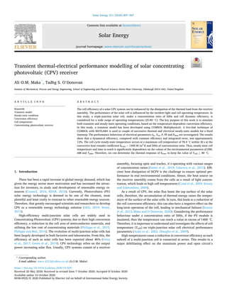
Fig. 1 illustrates the flowchart diagram describing the modelling
approach. The electrical model consists of a GaInP/GaInAs/Ge, triple-
junction cell, with a standard DNI = 1000 W/m2
and at CR = 500x,
which is detailed in Section 3.1. Temperature dependence has been
Nomenclature
Ac Area of the cell (m2
)
As Convective area (m2
)
CR Concentration Ratio (x)
DNI Direct Normal Irradiance (W/m2
)
G Solar direct irradiance (W/m2
/nm)
hconv Convection heat transfer coefficient (W/m2
K)
Jsc Short circuit current density (A/m2
)
Jo Dark current density (A)
kb Boltzmann constant (eV/K)
n Diode ideality factor (–)
q Electron charge (c)
qheat Heat power (W)
Rs Series resistance (Ω)
SR spectrum response (A/W)
∂T Temperature different
Δt Time different (s)
Tamb Ambient temperature (◦
C)
To Temperature at standard condition (◦
C)
Tc Cell temperature (◦
C)
Voc Open circuit voltage (V)
P Power (W)
Pmax. Maximum power (W)
T Time (s)
Greek symbols
ηopt Optical efficiency
σ Stefan–Boltzmann constant (W/(m2
K4
))
ε Surface emissivity (–)
ηc Cell efficiency
λ wavelength (nm)
α Material constant (eV/K)
β Material constant (K)
βη Efficiency temperature coefficient
γ Constant (–)
K Constant (A/(cm2
K4
))
Abbreviations
AM Air Mass
GaInP Gallium Indium Phosphide
GaInAs Gallium Indium Arsenide
Ge Germanium
EQE External Quantum Efficiency
FEM Finite Element Method
1D One-dimensional
3D Three-dimensional
FF Fill Factor
HCPV High Concentrating Photovoltaic
DBC Direct Bonded Copper
Al2O3 Aluminium Oxide
A.O.M. Maka and T.S. O’Donovan
3. Solar Energy 211 (2020) 897–907
899
predicted for cell efficiency and heat power generation from incident
solar power. The modelling results are compared with a commercial CPV
cell for temperature range 25–80 ◦
C.
The numerical simulation of the three-dimensional study with a
thermal model is coupled with an electrical model, which is detailed in
Section 3.2. The model was developed using MATLAB live-link to couple
the characteristics of the changing materials of the model for each
convergent and transient step. Initial cell temperature is modified after
each iteration, changing both the electrical conversion efficiency and
the rate of heat transfer from the cell. Steady-state is deemed to have
been achieved when the cell temperature remains constant with subse
quent iterations, indicating the conservation of energy has been satiated.
A transient model is a model that contains dependent variables that
changes over time and is used here to determine the effect of a changing
environment on the performance of a HCPV cell. Besides, this is known
as a dynamic model, time-dependent model or unsteady model (Multi
physics, 2012). The model proposed here is a sequence of several steady-
state conditions, where the initial condition of the iterative solution is
the final steady-state condition of the previous timestep, as shown in
Fig. 1.
3. Numerical modelling
3.1. Electrical model of triple-junction cells
The electrical model is the cornerstone of performance evaluation
and energy generation of PV solar cells. A solar cell is a semiconductor
material based on p-n junctions, designed to produce current by
absorbing the light of energy photons. Performance evaluation of solar
cells is dependent on parameters of voltage-current characteristics.
Triple-junction solar cells are made of III-V materials; it consists of three
subcell’s, GaInP/GaInAs/Ge, monolithically stacked. It is important to
determine the short current density generated by the cells, as given by
Eq. (1) (Peharz et al., 2009).
Jsc,i = CR.
∫ λ2
λ1
SRi(λ).ηopt(λ).G(λ).dλ (1)
where CR is a concentration ratio of 500x, and SR is the spectral
response and ηopt is the optic efficiency. Eq. (2) (known as the Shockley
diode equation) characterises the current produced by the solar cell:
J,i = Jph,i − J0,i
(
exp
q(V,i + J.Rs,i)
n.Kb.Tc
− 1
)
−
V,i + J.Rs,i
Rsh
(2)
where Rs is series resistance, V is the voltage, Rsh is the shunt resistance,
Jph is the photocurrent. In the ideal case, the photocurrent is equal to
short circuit density Jph = Jsc. The Rsh is of a magnitude that can be
neglected (Theristis and O’Donovan, 2015). The overall current is
determined by the light-induced current from the diode dark current and
is given by Eq. (3). The total current of the three subcells, in series
connection, is limited by lower current density and the total voltage will
be the sum of three subcells. The open-circuit voltage (Voc) can be given
by the relationship (4):
J,i = Jo,i
(
exp
q(V + J,i.Rs
n.Kb.Tc
− 1
)
− Jsc,i (3)
Voc,i =
n.Kb.Tc
q
ln
(
Jsc,i
J0,i
+ 1
)
(4)
where n is the diode ideality factor, Kb is Boltzmann constant, Tc is
temperature, q is the electron charge, Rs is a series resistance, and Jo is
the reverse saturation current. The voltage output of the entire cell is the
sum of the three subcells. The total current is determined by limiting the
lowest photocurrent generated by three subcells. The Fill Factor (FF) is
the ratio of the maximum output power, Pmax, from the solar cell,
divided by the open circuit voltage and short-circuits current density, as
given in Eq. (5):
FF =
Pmax
Voc.Jsc
=
Jmax.Vmax
Voc.Jsc
(5)
The electrical efficiency of the cell (ηel) is quantified by dividing
power output by power input as given by Eq.(6). Where Pout is a deliv
ered power and Pin is the amount of incident power in the solar cell.
ηel =
Pmax
Pin
=
Jsc.Voc.FF
pin
(6)
Cell efficiency ηc, as a function of temperature, can be calculated by
Eq. (7) (Ceylan et al., 2016; Sarhaddi et al., 2010). Where ηel is cell
electrical efficiency for the concentration ratio, βη is efficiency temper
ature coefficient, and To is reference condition temperature.
ηc(T) = ηel
[
1 − βη
(
T*
c − To
) ]
(7)
3.2. Thermal FEM model
Thermal FEM modelling utilises COMSOL Multiphysics, which is
iteratively solved by Partial Differential Equations (PDEs). In the FEM,
the simulation starts by producing the geometry and dividing it into
finite elements. The “Heat Transfer in Solids” simulation physics is used
to develop 1D and 3D dynamic thermal models.
The aluminium oxide interlayer offers electrical insulation between
the top and bottom subcell materials. The insulation materials in the
middle of the Direct Bonded Copper (DBC) sandwich between the bot
tom and top copper, as Al2O3 has excellent combined properties as an
electrical insulator and thermal conductor (García et al., 2016). To
simplify the model, the electrical terminals and bypass-diodes are not
considered.
For the optimum design of a CPV system from the perspective of
conversion efficiency, the level of temperatures of a CPV system should
be maintained as low as possible. Therefore, to implement a heat
transfer model, it is essential to design a system which can investigate
the variance in temperature and system performance. The thermal
design is built on our understanding of the processes of heat transfer,
Fig. 1. Flowchart of the modelling process.
A.O.M. Maka and T.S. O’Donovan
4. Solar Energy 211 (2020) 897–907
900
from assembly to unit level, by conduction, convection and radiation.
Eq.(8) (Aldossary et al., 2016; Theristis et al., 2012) expresses the heat
dissipation by conduction through the receiver of the solid component.
Where K is thermal conductivity, (∂T/∂x) is the temperature gradient, A
is conductive area and qcon is conduction heat transfer (W/m2
).
qcon = − K.A.
∂T
∂x
(8)
The amount of heat that is dissipated by convection from the surface
to the air is expressed in Eq. (9) (Theristis et al., 2012). Where qconv is
convection heat transfer (W/m2
), As is convective area, hconv is a con
vection heat transfer coefficient.
qconv = hconv.As.
∂T
∂x
(9)
The heat loss by radiation transferring heat by electromagnetic
waves to the environment is expressed by Eq. (10) (Theristis et al.,
2012). qrad is radiative heat flux (W/m2
), Ts is surface temperature, ε is
surface emissivity, and σ is the Stefan-Boltzmann constant.
qrad = ε.σ.A.(T4
s − T4
amb) (10)
Thermal equilibrium with the surrounding environment occurs in
the electronic device when it is not under operating conditions and at
the same temperature of the surrounding media. Although, when the
device is active, the component’s, and the solar cell device, the tem
perature begins to increase due to the absorption of heat, the tempera
ture of the device stabilises at the point when the heat generated equals
the heat released throughout the cooling mechanism. At that point, the
device has reached steady-state operating conditions. The period during
the warming-up, when the component temperature rises, is called the
operational transient period (Cengel, 1998).
3.3. Receiver geometry and boundary condition
The boundary conditions in the solid domains are applied. The model
geometry of a receiver assembly is attached to a Direct Bonded Copper
(DBC) carrier, made of copper/Al2O3 ceramic/copper. The receiver
configuration set at the bottom convective area is about 5.13 × 10− 4
m2
,
and the solar cell area is 1 cm2
. Using the multi-junction solar cell’s heat
source at CR = 500x, the heat power is generated by the portion that is
not converted to electricity. Heat transfer in the solid-state is due to the
material’s thermal properties. A convective heat transfer boundary
condition has been applied to the backside of the plate, hconv = 1400 W/
m2
K. The ambient temperature around the receiver was set to 25 ◦
C. The
optimum geometry mesh of normal size, free triangle type was applied.
Fig. 2 shows a 3D receiver structure, and the selected point at the centre
of the cell for the 1D single plot. Table 1 listed the single CPV receiver
assembly dimensions.
4. Results and discussions
4.1. Temperature dependent on cell efficiency
The solar cell generates heat and electrical energy at high optical
concentrations. In a series connection, the PV module’s efficiency is
limited as its temperature increases. A solar receiver assembly usually
contains a bypass diode, which will override the cell to avoid over
heating, which leads to a reduction in cell/module efficiency (Broderick
et al., 2015; Helmers et al., 2013).
The current model accounts for the temperature dependence of the
solar cell’s efficiency and the effects of temperature from 25 to 80 ◦
C and
CR = 500x; the trends of efficiency decrease linearly as the temperature
increases. The normalised temperature coefficients of the conversion
efficiency (Δη/dT) of the triple-junction solar cell is 0.047%/K (Azur
space, 2014). The variation of efficiency with temperature is shown as a
linear relationship between temperature and efficiency, as illustrated in
Fig. 3.
This study considered the transient response to a step input, from
unilluminated to being subjected to concentrated (500x) sunlight.
During the process of solar concentration, the uniform light of solar
radiation is concentrated onto a small area. The thermal gradient is
affected by the temperature difference between the edge, and centre, of
the solar cell. That is due to the difference in heat dissipation from
conduction and convection heat transfer (Cotal and Frost, 2010; Rey-
Stolle et al., 2016).
Initially, as the cell temperature rises, the cell material’s band gap
decreases, hence a larger portion of the incident spectrum can be
absorbed by the hottest region. The effect of the temperature rises is a
decrease in the operating efficiency of the solar cells. The current
mismatch can happen between several regions of a cell operating at
different temperatures. The generation of thermal energy at every sub
cell in GaInP/GaInAs/Ge triple-junction solar cells is higher in the bot
tom subcell Ge (Sharpe et al., 2013).
4.2. Validation
This proposed model is verified by using data from a commercial PV
cell. It is typically used in CPV, the conversion efficiency as a function of
Fig. 2. 3D structure of receiver assembly.
Table 1
Dimensions of CPV receiver assembly (Theristis and O’Donovan, 2015).
Receiver layer Width (mm) Thickness (mm) Length (mm)
Solar cell 10 0.19 10
Copper 19.5 0.25 24
Al2O3 21 0.32 25.5
Copper 20.5 0.25 25
Fig. 3. Temperature-dependent on cell efficiency as a function of temperature-
dependence from 25 to 80 ◦
C and at CR of 500x.
A.O.M. Maka and T.S. O’Donovan
5. Solar Energy 211 (2020) 897–907
901
temperature from 25 to 80 ◦
C versus different values of concentration
ratios. Hence, the performance measurement data is presented by AZUR-
SPACE Solar Power GmbH, as shown in Fig. 4 (Azurspace, 2014).
Table 2 summarises a comparison between this study, modelling and
measurement at CR = 500x of efficiency at a temperature of 25 ◦
C. The
results show disparities emerging; therefore, the efficiency deviation is
about 0.8%, found at 25 ◦
C, and about 2.5% at a temperature of 80 ◦
C.
Furthermore, as depicted in Fig. 4, as sunlight concentration in
creases, the efficiencies decrease to a certain level. Hence, the behaviour
can be explained by a reduction in series resistance as temperature rises
(Ghoneim et al., 2018; Helmers et al., 2013). Moreover, as the FF de
creases owing to series losses, the efficiency degendered to a certain
level (Fernández et al., 2018).
4.3. Heat power
The main reason for the decrease in cell efficiency at high concen
trations is attributed to the temperature rise. The heat power (or heat
flux), is the heat generated on the top of the solar cells as a result of
optical concentration. The heat power, as a function of temperature, is
considered in this study for a temperature range from 25 to 80 ◦
C. Under
concentration, the heat power generated by the solar cell is quantified
by the given Eq. (11) (Fernández et al., 2014; Ota et al., 2013).
qheat(T) = DNI.(1 − ηc)Ac.CR.ηopt (11)
Temperature-dependence of heat power can be predicted (qheat)
based on the efficiency temperature dependence. It indicates that a
decrease in heat power due to an efficiency drop increases temperature,
as shown in Fig. 5. The DNI is taken as a constant value of 1000 W/m2
and AM 1.5D; the ɳc is variable with cell efficiency as a function of
temperature.
4.4. Thermal response analysis
In this simulation, the model is run twice: once by using a stationary
cell efficiency study, and another by dynamic cell efficiency. The values
of dynamic efficiency are variable from 40.4 to 36%. Thus, the time-
dependent model is beneficial in comprehending the heating time
required by the cell to reach the steady-state condition. The dynamic
model comprises of a series of steady-state models, where the time-step
between successive steady-state models becomes a factor.
Based on the FEM model, the initial and boundary conditions are set.
As a result, electrical efficiency decreases as a function of temperature,
which corresponds to the increase in heat power generated. Therefore,
this approach gives an overview of understanding the device’s transient
performance. Most of the heat is densely focused in the centre of the
solar cell and decreases gradually towards the receiver assembly edge.
Fig. 6 shows a graph of steady-state temperature against time, for three
values of the timestep, Δt (1,5,10 s). Hence, the time-dependent study,
where a timestep is set, represents the time differences between each
iteration until the end of the computation. As the temperature and
corresponding efficiency varies significantly within the larger timesteps,
it is clear that the timestep must be maintained at or below 1 s to
accurately predict the performance of the cell to a step-change in solar
flux.
In this model, we consider a uniform illumination on the cell surface.
The actual heat dissipation distribution is non-uniform across the
receiver. Basically, the heat is transferred through the PV cell’s solid
layers by conduction. Thus, the heat conduction is most intense at the
cell’s centre, although, at the edge of the cell, conduction and radiation
heat transfer does take place. Eventually, the heat is dissipated to the
surrounding environment by convection and radiation heat transfer.
500x
Fig. 4. Measured data of performance curve for 3C42A, 2014 by AZUR-SPACE
Solar Power GmbH; for concentration ratio from 100 to 1500x versus the
conversion efficiency with a variable operating temperature from 25 to 80 ◦
C
(Azurspace, 2014).
Table 2
Comparison of cell efficiency resulting from this modelling and between
experimental data extracted from 3C42A, AZUR-SPACE and current model at
500x.
Temperature
(◦
C)
3C42A ηc (Azurspace,
2014).
Current model
ηc
Deviations
(%)
25 ◦
C 41.2% 40.4% 0.8
80 ◦
C 38.5% 36% 2.5
Fig. 5. Temperature-dependence on the heat power generated by the cells of
temperature from 25 to 80 ◦
C.
Fig. 6. Transient model results and steady-state temperature against time for
three values of the timestep.
A.O.M. Maka and T.S. O’Donovan
6. Solar Energy 211 (2020) 897–907
902
The error ratio between the dynamic efficiency with constant effi
ciency is calculated. Integrated Error (IE) from (0–60 s) is about 12%,
from an initial temperature of 25 ◦
C to a steady-state temperature, which
occurred at around 30 s; hence, the maximum cell temperature is
78.4 ◦
C. The Maximum Error Point (MEP) is about 24% and occurs at 10
s. In this model, cell temperature loops until reaching a steady-state,
although that steady-state occurs when the transient cell temperature
(Tcell) trends, and adjacent cell temperature, the trend tends to 0%, with
a stationery efficiency of 36% and the initial temperature of 25 ◦
C. Fig. 7
shows the results of the comparison between the steady-state tempera
ture for both constant and dynamic efficiency.
The receiver assembly is simulated for time intervals from 0 to 30 s.
Fig. 8 illustrates the resulting temperature distribution across the cell
and receiver assembly for t = 0 s to t = 30 s at 5 s intervals (CR = 500x
and hconv = 1400 W/m2
K). The thermal management of the assembly is
reliant on convection from the back of the receiver and the environ
mental conditions. Fig. 8(a) represents the initial cycle simulation when
t = 0 s; hence, the cell temperature is about 25 ◦
C. In Fig. 8(b), there was
a little increase of cell temperature at t = 5 s, and the maximum cell
temperature is shown densely on the centre of the cell and stagnated at
35.5 ◦
C, but the edge of the cell has the temperature about 28 ◦
C.
In Fig. 8(c) the temperature is increased to reach 45.6 ◦
C at t = 10 s;
temperature distribution pattern on the cell increased at the edge to
about 40 ◦
C. In Fig. 8(d) the temperature of the cell rises to 55.5 ◦
C at t =
15 s, and here the temperature of Direct Bonded Copper (DBC) carrier
started increasing to reach 34.6 ◦
C. In Fig. 8(e) the cell temperature
increased to reach 65.5 ◦
C at t = 20 s, and the (DBC) carrier temperature
was about 43.8 ◦
C. In Fig. 8(f) at t = 25 s, the cell temperature increased
to reach 75.5 ◦
C, and on the attached (DBC) carrier, the temperature was
approximately 53 ◦
C. Lastly, Fig. 8(g) represents the movement from
transient to the steady-state condition at t = 30 s: the cell temperature
was about 74.4 ◦
C and the pattern temperature distribution on the
attached (DBC) carrier, was from 55 to 65 ◦
C.
It is cleared that the thermal response of the cell and assembly varies
significantly over the 30 s period. Also, if effective and cost-effective
thermal management systems are to be designed to optimise the elec
trical conversion efficiency, and consequently the electrical yield of the
system, then dynamic modelling is important (Migliorini et al., 2017).
By comparison, a three-dimensional model (3D) of temperature
profile distribution on a multijunction solar cells receiver, presented in
Fig. 9, shows results for constant efficiency. For a time period of 0–60 s,
the constant efficiency used in this model is approximately 36%, the cell
temperature is about 78.4 ◦
C, and occurs at 30 s. The attached (DBC)
carrier shows a variable temperature distribution pattern ranging from
55.1 to 66 ◦
C. The final maximum cell temperature at dynamic efficiency
was similar and therefore reached the steady-state condition at the same
time, within 30 s, in the constant efficiency.
In the three-dimensional model, the temperature distribution of the
triple-junction cell needs an accurate light profile, since overall input
with comprehensive information on a material temperature is depen
dent on parameters such as energy band gap, absorption, etc. (for
semiconductor materials with a stack of multi-junction). Hence, the
presence of the 3D model will help in predicting regions of the solar cell,
which have malfunctions as an effect of high temperatures (Rey-Stolle
et al., 2016).
4.5. Analysis of electrical parameters response
In steady-state conditions, the entire heat generated by the assembly
is transferred to the ambient environment. Thus, the optimum thermal
management mechanisms reported for CPV application at 500x might
include a heat spreader, heat sink, micro-channel, jet impingement and
liquid immersion etc. Here, a rear surface convective heat transfer co
efficient of 1400 W/m2
K and an ambient temperature of 25 ◦
C was
considered, and the predicted cell temperature is approximated to be
78.92 ◦
C (Jakhar et al., 2016).
The cell performance is very sensitive to temperature increases,
which are simulated in transient methods. In Fig. 10, when the solar
cell’s performance parameters are decreased as temperatures increases,
the temperature dependence on the short-circuit current density (Jsc)
slightly increases over time until the temperature reaches a steady-state
at 30 s, as shown in Fig. 10(a). This behaviour can be explained where,
as the temperature increases, the energy band gap decreases, as more
solar spectrum photon components are absorbed. Subsequently, this
leads to a slight increase in short circuit current density.
The temperature dependence on the open circuit’s voltage (Voc)
decreases over time, as shown in Fig. 10b). As a result of rising cell
temperature, the effects of Voc gradually decreased from 3.01 to 2.84 V.
The fill factor, also, decreases as cell temperature increases as shown in
(Fig. 10(c)). The FF depends on the energy band gap of the cell materials,
which is affected more by temperature increases. Therefore, it steadily
decreases from 0.84 to 0.78 and stabilises within 30 s. The maximum
power point also drops as cell temperature increases with time until
stagnation temperature stabilises as shown in (Fig. 10(d)). The
maximum power (Pmax) of the cell is gradually decreasing from 19 to
16.7 W and reaches a steady-state within 30 s.
Fig. 11(b) illustrates the overall solar cell’s conversion efficiency
using the time-dependent temperature, where it tends to decrease to
wards a steady-state. The efficiency in a time-dependent pattern drops
from 40.4% (at 0 s) to a steady-state efficiency of about 36.4%, which
occurs within 30 s. Therefore, this high temperature proves it is the
cause of the decrease in the conversion efficiency; the details of that are
observed on the process of dynamic losses.
Fig. 11(a) represents the power output during the transient and the
steady-state condition. As a result of reductions on the parameters of Voc,
FF and Pamx., when cell temperature rises, the output power also will
drop to a certain level. Hence, the shown output power gradually de
creases from 18.7 to 16.5 W and stabilises within 30 s. Based on that, the
steady-state output power is fundamental to predicting energy yield
gained from the cell/module/system.
4.6. Effects of varying irradiance intensity in steady-state cell temperature
Knowing the temperature behaviour of multi-junction solar cells for
various irradiations is essential for both the Earth concentrator appli
cations and space applications (Helmers et al., 2013). Despite the impact
of temperature on HCPV operating performance and system integrity,
the modelling technique used predicts the range of operating tempera
ture for various environmental conditions, including irradiance and
environment temperature etc.
The performance of the solar cell is influenced by incident illumi
nation and its operating temperature. Fig. 12 depicts the solar cell
Fig. 7. Transient model results in steady-state maximum temperature for both
constant efficiency and dynamic efficiency.
A.O.M. Maka and T.S. O’Donovan
7. Solar Energy 211 (2020) 897–907
903
steady-state temperature versus different values of DNI, the optimum
time-dependent, selected at Δt = 1(s). With the high irradiance intensity
of 1000 W/m2
, the steady-state cell temperature was 78.4 ◦
C at the time
of 30 s. Hence, at an irradiance intensity of 700 W/m2
, the steady-state
temperature was about 67.5 ◦
C at the time of 25 s. Although, at low
values of irradiance intensity of 400 W/m2
, steady-state cell tempera
ture was 56.1 ◦
C at approximately 20 s. This behaviour can be explained,
since the slopes of the three case curves are identical, from the initial up
Fig. 8. 3D Temperature profile distribution patterns and cell steady-state temperature of the dynamic efficiency of receiver assembly for different intervals as listed
in (a, b, c, d, e, f, g) and steady-state time listed respectively (0, 5, 10, 15, 20, 25, 30 s).
A.O.M. Maka and T.S. O’Donovan
8. Solar Energy 211 (2020) 897–907
904
to a certain level, as they have a fixed set-up of Tamb = 25 ◦
C and hconv =
1400 W/m2
K. On the other hand, the achieved values of steady-state
cell temperature are different here, due to the various values of the
DNI and corresponding AM.
The irradiance intensity has a significant influence on steady-state
cell temperature. As the values of DNI changes at conditions of (1000
W/m2
, 700 W/m2
, 400 W/m2
) the slope linearly increases; the regres
sion was (R2
= 0.9996). The predicted cell temperature was variable
(between 78.4 and 56.1 ◦
C), the cell efficiency decreased sharply from
36.4% to 32.3%, as illustrated in Fig. 13. The cell steady-state temper
ature response remarkably shows the effect of increases and decreases of
DNI at the steady-state cell temperature. It’s important here to mention
that 1000 W/m2
of the DNI and corresponding AM represents the
midday operating condition, which is approximately the maximum
values during the operation. In contrast, 400 W/m2
of the DNI and
corresponding AM represents the period of sunrise/sunset, which are the
lowest values.
In summary, as shown, the increase of DNI leads to an increase in cell
temperature as a result of increased heat flux and a reduction in con
version efficiency. Table 3 also summarised the comparison of different
DNI steady-states values. Nonetheless, to be considered on a daily basis,
the DNI values are variable between sunrise, midday and sunset; the
cell’s operating performance behaviour will change accordingly.
Fig. 14 illustrates the different values of DNI and their corresponding
values of AM. As is significantly shown in Fig. 14, there is a directly
proportional relationship between these two parameters. The AM is a
measure of the atmospheric depth crossed by solar radiation. Also, the
AM had significant effects on the wavelengths of solar radiation. In the
real operating conditions daily, the values of AM and DNI are variable,
from sunrise to sunset, and will be considered in future work.
4.7. Effects of varying ambient temperature in the steady-state cell
temperature
The factor which is essential when considering the PV cell temper
ature is the ambient temperature, with regards to the variability of
ambient temperature and its effect on the solar cell’s steady-state tem
perature. In this scenario, when the DNI = 1000 W/m2
and the ambient
temperature Tamb = 25 ◦
C, the steady-state cell temperature is 78.4 ◦
C
for hconv = 1400 W/m2
K. Furthermore, for Tamb = 35 ◦
C, the steady-
state cell temperature is about 78.8 ◦
C and the response of hconv =
1500 W/m2
. For Tamb = 45 ◦
C, the steady-state cell temperature is about
79.2 ◦
C and the response of hconv = 1600 W/m2
K. Fig. 15 illustrates the
steady-state cell temperature at a variety of ambient temperatures. This
behaviour can be explained by the higher heat transfer coefficient
Fig. 9. 3D temperature profile distribution, steady-state model at con
stant efficiency.
Fig. 10. Electrical performance parameters of transient and cell steady-state condition. (a) short current density versus time, (b) open circuit voltage versus time, (c)
fill factor versus time, (d) maximum power point versus time intervals.
A.O.M. Maka and T.S. O’Donovan
9. Solar Energy 211 (2020) 897–907
905
leading to lower thermal resistance, which in turn lowers the operating
temperature of the CPV cell/module.
The predicted model can provide monitoring of the devices in order
to have a better understanding of performance behaviour, which will
enable proper selection of appropriate solutions for heat dissipation.
Hence, transient analysis of the thermal and electrical behaviour is
performed, and these collected notifications will be used to provide
improved knowledge of CPV performance behaviour. The techniques to
limit the influence of the operating temperature of the internal device
are not assessed; it needs more advanced tools for accurate prediction.
5. Conclusions
In this work, a model was developed to characterise the transient
thermal and electrical performance of triple-junction solar cells. The
transient model here is used to comprehend the transient state during
operating conditions. Consequently, it is significant to our understand
ing of operating performance behaviour, and it is a step towards
enhancing the device design. The conclusions of this work are sum
marised below as follows:
• It has been established that a time step, Δt of 1 s is required for the
range of parameters studied, to accurately predict cell performance.
Through the dynamic model, the impact of different incident solar
0 10 20 30 40 50 60
34
35
36
37
38
39
40
41
Conversion
efficiency
(%)
Time (s)
(a)
(b)
Fig. 11. (a) Power output versus transient and steady-state conditions, (b)
Conversion efficiency versus cell transient and steady-state conditions.
Fig. 12. Effects of changes DNI in the cell temperature at dynamic efficiency for
time for steady-state temperature.
Fig. 13. Different values of DNI versus cell temperature at steady-state
temperatures.
Table 3
Detailed variation of DNI for maximum cell temperature, steady-state conver
sion efficiency and time.
Parameters DNI = 1000 (W/
m2
)
DNI = 700 (W/
m2
)
DNI = 400 (W/
m2
)
Steady-state Tcell
(◦
C)
78.4 67.5 56.1
Steady-state (ɳc) 36.4 34.5 32
Steady-state time
(s)
30 25 20
Fig. 14. Different values of DNI various the corresponding values of AM.
A.O.M. Maka and T.S. O’Donovan
10. Solar Energy 211 (2020) 897–907
906
flux values on the power output of the photovoltaic device could also
be determined. A dynamic efficiency compared with constant effi
ciency, and integrated error is about 12%.
• The comparison of the cell temperatures ranging from 25 to 80 ◦
C is
reported. The difference in the efficiency of approximately 0.8% is
found for lower temperatures, and this rises to approximately 2.5%
for the higher temperatures within the range considered.
• Cell steady-state temperature occurs at a maximum cell temperature
of 78.4 ◦
C within the 30 s, at convective heat transfer coefficient
hconv = 1400 W/m2
K and concentration ratio CR = 500x. Further
more, in scenario of Tamb = 35 ◦
C, the steady-state cell temperature is
about 78.8 ◦
C and the thermal response of hconv = 1500 W/m2
. For
Tamb = 45 ◦
C, the steady-state cell temperature is about 79.2 ◦
C and
the thermal response of hconv = 1600 W/m2
K. Thus, as deduced at
high ambient temperature, there will be a requirement for high
convective heat transfer coefficients to maintain a cell operating
temperature below 80 ◦
C.
• The higher value of DNI 1000 W/m2
and the corresponding lower
value of AM represents the midday operating condition, which is
approximately the maximum values during the operation. The
steady-state cell temperature was 78.4 ◦
C at the time of 30 s. In
contrast, lower values of DNI 400 W/m2
and the corresponding
higher value of AM represents the period of sunrise/sunset, which
are the lowest values. The steady-state cell temperature was 56.1 ◦
C
at approximately 20 s.
• The present study contributes to the understanding of the transient
state, that lies in the link between the ideal modelling and environ
mental operating conditions. Consequently, that is very significant in
our comprehension of the transient nature of CPV receivers.
Based on the approaches mentioned above and outcomes, in the
future, it is recommended that research studies include dynamic per
formance measuring/modelling for both small and large-scale opera
tions with consideration to the weather and environmental data.
Declaration of Competing Interest
The authors declare that they have no known competing financial
interests or personal relationships that could have appeared to influence
the work reported in this paper.
Acknowledgement
Many grateful thanks to the School of Engineering and Physical
Sciences, Heriot-Watt University, United Kingdom, also many thanks to
Libyan Authority for Research Science and Technology.
References
AEO, 2019. Annual Energy Outlook with projections to 2050. January 24, 2019 www.
eia.gov/aeo.
Aldossary, A., Mahmoud, S., Al-Dadah, R., 2016. Technical feasibility study of passive
and active cooling for concentrator PV in harsh environment. Appl. Therm. Eng. 100,
490–500.
Araki, K., Uozumi, H., Yamaguchi, M., 2002. A simple passive cooling structure and its
heat analysis for 500/spl times/concentrator PV module. In: Photovoltaic Specialists
Conference, 2002. Conference Record of the Twenty-Ninth IEEE. IEEE, pp.
1568–1571.
Azurspace, 2014. Triple junction solar cell assembly – Type 3C42A. data sheet.
Broderick, L.Z., Albert, B.R., Pearson, B.S., Kimerling, L.C., Michel, J., Cells, S., 2015.
Design for energy: Modeling of spectrum, temperature and device structure
dependences of solar cell energy production. Sol. Ener. Mater. Sol. Cells. 136, 48–63.
Cengel, Y.A., 1998. Heat Transfer: A Practical Approach. WBC McGraw-Hill.
Ceylan, İ., Gürel, A.E., Ergün, A., Tabak, A., 2016. Performance analysis of a
concentrated photovoltaic and thermal system. Sol. Energy 129, 217–223.
Cotal, H., Fetzer, C., Boisvert, J., Kinsey, G., King, R., Hebert, P., Yoon, H., Karam, N.,
2009. III–V multijunction solar cells for concentrating photovoltaics. Ener. & Enviro.
Sci. 2 (2), 174–192.
Cotal, H., Frost, J., 2010. Heat transfer modeling of concentrator multijunction solar cell
assemblies using finite difference techniques. In: Photovoltaic Specialists Conference
(PVSC), 2010 35th IEEE. IEEE, pp. 000213–000218.
Cotal, H., Sherif, R., 2006. Temperature dependence of the IV parameters from triple
junction GaInP/InGaAs/Ge concentrator solar cells. In: Photovoltaic Energy
Conversion, Conference Record of the 2006 IEEE 4th World Conference on. IEEE,
pp. 845–848.
Council, W.E., 2016. World Energy Resources 2016. World Energy Council, London, UK.
Fernández, E.F., Almonacid, F., Rodrigo, P.M., Pérez-Higueras, P.J., 2018. CPV Systems,
McEvoy’s Handbook of Photovoltaics. Elsevier, pp. 931–985.
Fernández, E.F., Rodrigo, P., Almonacid, F., Pérez-Higueras, P., 2014. A method for
estimating cell temperature at the maximum power point of a HCPV module under
actual operating conditions. Sol. Ener. Mater. Sol. Cells. 124, 159–165.
García, I., Victoria, M., Antón, I., 2016. Temperature effects on CPV solar cells, optics and
modules. Handbook Concentrat. Photovoltaic Technol. 245.
Geisz, J.F., Steiner, M.A., Jain, N., Schulte, K.L., France, R.M., McMahon, W.E., Perl, E.E.,
Friedman, D.P., 2017. Building a six-junction inverted metamorphic concentrator
solar cell. IEEE J. Photovolt. 8 (2), 626–632.
Ghoneim, A.A., Kandil, K.M., Alzanki, T.H., Alenezi, M., 2018. Performance analysis of
high-concentrated multi-junction solar cells in hot climate. Int. J. Sustain. Energy 37
(3), 294–310.
Green, M.A., Dunlop, E.D., Levi, D.H., Hohl-Ebinger, J., Yoshita, M., Ho-Baillie, A.W,
applications, 2019. Solar cell efficiency tables (version 54). 27(7), 565–575.
Helmers, H., Schachtner, M., Bett, A.W., Cells, S., 2013. Influence of temperature and
irradiance on triple-junction solar subcells. Sol. Energ. Mater. Sol. Cells. 116,
144–152.
Jakhar, S., Soni, M., Gakkhar, N., 2016. Historical and recent development of
concentrating photovoltaic cooling technologies. Renew. Sustain. Energy Rev. 60,
41–59.
Kinsey, G.S., Edmondson, K.M., 2009. Spectral response and energy output of
concentrator multijunction solar cells. Prog. Photovoltaics Res. Appl. 17 (5),
279–288.
Kumar, N.S., Matty, K., Rita, E., Simon, W., Ortrun, A., Alex, C., Roland, W., Tim, G.,
Kumar, M.T., 2012. Experimental validation of a heat transfer model for
concentrating photovoltaic system. Appl. Therm. Eng. 33, 175–182.
Maka, A.O., O’Donovan, T.S., 2020. A review of thermal load and performance
characterisation of a high concentrating photovoltaic (HCPV) solar receiver
assembly. Sol. Energy 206, 35–51.
Maka, A.O., O’Donovan, T.S., 2019a. Analysis of thermal response and electrical
characterisation of triple-junction solar cells based on variable solar spectral
irradiance and air mass. Therm. Sci. Eng. Prog. 10, 269–279.
Maka, A.O., O’Donovan, T.S., 2019b. Modelling of the thermal behaviour of solar high
concentrating photovoltaic receiver. Therm. Sci. Eng. Prog. 9, 281–288.
Migliorini, L., Molinaroli, L., Simonetti, R., Manzolini, G., 2017. Development and
experimental validation of a comprehensive thermoelectric dynamic model of
photovoltaic modules. Sol. Energy 144, 489–501.
Muller, M., Kurtz, S., Steiner, M., Siefer, G., 2015. Translating outdoor CPV I-V
measurements to a CSTC power rating and the associated uncertainty. Prog.
Photovolt.: Res. Appl. 23 (11), 1557–1571.
Multiphysics, C., 2012. COMSOL multiphysics user guide (Version 4.3 a). COMSOL, AB,
39–40.
Muron, A., Chow, S., Wheeldon, J., Hinzer, K., Schriemer, H., 2011. Thermal
optimization of a solar cell carrier for concentrator systems. In: Photonics North
2011. International Society for Optics and Photonics, pp. 800722.
Nishioka, K., Sueto, T., Uchida, M., Ota, Y., 2010. Detailed analysis of temperature
characteristics of an InGaP/InGaAs/Ge triple-junction solar cell. J. Electron. Mater.
39 (6), 704–708.
Ota, Y., Nagai, H., Araki, K., Nishioka, K., 2013. Thermal transfer simulation for
concentrator photovoltaic receiver under concentration condition. In: 9th
International Conference On Concentrator Photovoltaic Systems: CPV-9. AIP
Publishing, pp. 18–21.
Fig. 15. Effects of different ambient temperature on the steady-state cell
temperature in order to maintain the temperature below a safe level and the
response of convection heat transfer coefficient.
A.O.M. Maka and T.S. O’Donovan
11. Solar Energy 211 (2020) 897–907
907
Peharz, G., Siefer, G., Bett, A., 2009. A simple method for quantifying spectral impacts on
multi-junction solar cells. Sol. Energy 83 (9), 1588–1598.
Philipps, S.P., Bett, A.W., Horowitz, K., Kurtz, S., 2015. Current status of concentrator
photovoltaic (CPV) technology. National Renewable Energy Lab. (NREL), Golden,
CO (United States).
Philipps, S.P., Bett, A.W.J., 2014. III-V Multi-junction solar cells and concentrating
photovoltaic (CPV) systems. Advan. Opt. Technolog. 3 (5–6), 469–478.
REGR, 2018 Renewables Energy Global status Report - REN21. www.ren21.net/wp-
content/.../2018/06/17-8652_GSR2018_FullReport_web_final_.pdf.
Rey-Stolle, I., Olson, J.M., Algora, C., 2016. Concentrator Multijunction Solar Cells.
Handbook on Concentrator Photovoltaic Technology, 59.
Sarhaddi, F., Farahat, S., Ajam, H., Behzadmehr, A., Adeli, M.M., 2010. An improved
thermal and electrical model for a solar photovoltaic thermal (PV/T) air collector.
Appl. Energy 87 (7), 2328–2339.
Sharpe, A., Eames, P., Dimroth, F., Araki, K., Antón, I., 2013. Modelling of multijunction
cell temperature distributions subject to realistic operating conditions. In: AIP
Conference Proceedings. AIP, pp. 142–146.
Sweet, T.K.N., Rolley, M.H., Li, W., Paul, M.C., Johnson, A., Davies, J.I., Tuley, R.,
Simpson, K., Almonacid, F.M., Fernández, E.F., 2018. Design and characterization of
hybrid III–V concentrator photovoltaic–thermoelectric receivers under primary and
secondary optical elements. Appl. Energy 226, 772–783.
Talavera, D., Pérez-Higueras, P., Ruíz-Arias, J., Fernández, E., 2015. Levelised cost of
electricity in high concentrated photovoltaic grid connected systems: spatial analysis
of Spain. Appl. Energy 151, 49–59.
Theristis, M., O’Donovan, T.S., 2015. Electrical-thermal analysis of III–V triple-junction
solar cells under variable spectra and ambient temperatures. Sol. Energy 118,
533–546.
Theristis, M., Sarmah, N., Mallick, T.K., O’Donovan, T.S., 2012. Design and numerical
analysis of enhanced cooling techniques for a high concentration photovoltaic
(HCPV) system. In: 27th European Photovoltaic Solar Energy Conference and
Exhibition. pp. 260–265.
Torres-Lobera, D., Valkealahti, S., 2014. Inclusive dynamic thermal and electric
simulation model of solar PV systems under varying atmospheric conditions. Sol.
Energy 105, 632–647.
Wang, N.-Y., Chiang, S.-Y., Chou, T.-L., Shih, Z.-H., Hong, H.-F., Chiang, K.-N., 2010.
Transient thermal analysis of high-concentration photovoltaic cell module subjected
to coupled thermal and power cycling test conditions. In: Thermal and
Thermomechanical Phenomena in Electronic Systems (ITherm), 2010 12th IEEE
Intersociety Conference on. IEEE, pp. 1–6.
Watts, R.G., 2013. Engineering Response to Climate Change. CRC Press.
Zhangbo, Y., Qifen, L., Qunzhi, Z., Weiguo, P., 2009. The cooling technology of solar cells
under concentrated system. In: Power Electronics and Motion Control Conference,
2009. IPEMC’09. IEEE 6th International. IEEE, pp. 2193–2197.
A.O.M. Maka and T.S. O’Donovan