hypothesis testing

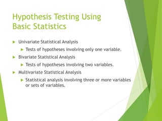
1. Hypothesis Testing Using
Basic Statistics
 Univariate Statistical Analysis
 Tests of hypotheses involving only one variable.
 Bivariate Statistical Analysis
 Tests of hypotheses involving two variables.
 Multivariate Statistical Analysis
 Statistical analysis involving three or more variables
or sets of variables.

2. Hypothesis Testing Procedure
 Process
 The specifically stated hypothesis is derived from the
research objectives.
 A sample is obtained and the relevant variable is
measured.
 The measured sample value is compared to the value
either stated explicitly or implied in the hypothesis.
 If the value is consistent with the hypothesis, the
hypothesis is supported.
 If the value is not consistent with the hypothesis,
the hypothesis is not supported.

3. Hypothesis Testing Procedure,
Cont.
 H0 – Null Hypothesis
 “There is no significant difference/relationship
between groups”
 Ha – Alternative Hypothesis
 “There is a significant difference/relationship between
groups”
 Always state your Hypothesis/es in the Null form
 The object of the research is to either reject or accept
the Null Hypothesis/es

4. Significance Levels and p-
values
 Significance Level
 A critical probability associated with a statistical
hypothesis test that indicates how likely an inference
supporting a difference between an observed value
and some statistical expectation is true.
 The acceptable level of Type I error.
 p-value
 Probability value, or the observed or computed
significance level.
 p-values are compared to significance levels to test
hypotheses.

5. Experimental Research: What
happens?
An hypothesis (educated guess) and then tested. Possible outcomes:
Something
Will Happen
It Happens
Something
Will Happen
It Does Not
Happen
Something Not
Will Happen
It Happens
Something
Will Not
Happen
It Does Not
Happen

6. Type I and Type II Errors
 Type I Error
 An error caused by rejecting the null hypothesis when
it should be accepted (false positive).
 Has a probability of alpha (α).
 Practically, a Type I error occurs when the researcher
concludes that a relationship or difference exists in
the population when in reality it does not exist.
 “There really are no monsters under the bed.”

7. Type I and Type II Errors
(cont’d)
 Type II Error
 An error caused by failing to reject the null
hypothesis when the hypothesis should be
rejected (false negative).
 Has a probability of beta (β).
 Practically, a Type II error occurs when a
researcher concludes that no relationship or
difference exists when in fact one does exist.
 “There really are monsters under the bed.”

8. Type I and II Errors and Fire
Alarms?
NO FIRE
FIRE
NO ALARM
Alarm
NO ERROR
NO ERROR
TYPE I
TYPE II
H0 is
True
H0 is
False
REJECT H0
ACCEPT H0
NO ERROR
NO ERROR TYPE II
TYPE I

9. Type I and Type II Errors -
Sensitivity
TYPE I TYPE II
Not Sensitive Sensitive

10. Normal Distribution
68%
95%
95%
99% 99%
.01 .01
.05 .05

11. Recapitulation of the Research
Process
 Collect Data
 Run Descriptive Statistics
 Develop Null Hypothesis/es
 Determine the Type of Data
 Determine the Type of Test/s (based on type of
data)
 If test produces a significant p-value, REJECT the
Null Hypothesis. If the test does not produce a
significant p-value, ACCEPT the Null Hypothesis.
 Remember that, due to error, statistical tests only
support hypotheses and can NOT prove a
phenomenon

12. Data Type v. Statistics Used
Data Type Statistics Used
Nominal Frequency, percentages, modes
Ordinal Frequency, percentages, modes,
median, range, percentile, ranking
Interval Frequency, percentages, modes,
median, range, percentile, ranking
average, variance, SD, t-tests,
ANOVAs, Pearson Rs, regression
Ratio Frequency, percentages, modes,
median, range, percentile, ranking
average, variance, SD, t-tests,
ratios, ANOVAs, Pearson Rs,
regression

13. Pearson R Correlation
Coefficient
X
1
3
5
5
1
2
4
6
Y
4
6
10
12
13
3
3
8

14. Pearson R Correlation
Coefficient
X Y 𝒙 − 𝒙 y −𝒚 xy 𝒙𝟐 𝒚𝟐
1 4 -3 -5 15 9 25
3 6 -1 -3 3 1 9
5 10 1 1 1 1 1
5 12 1 3 3 1 9
1 13 2 4 8 4 16
Total 20 45 0 0 30 16 60
Mean 4 9 0 0 6
A measure of how well a linear equation describes the
relation between two variables X and Y measured on
the same object

15. Calculation of Pearson R
–regression-
𝑟 =
𝑥𝑦
𝑥2 𝑦2
𝑟 =
30
16 60
=
30
960
=
30
30.984
= 0.968

16. Alternative Formula
𝑟 =
𝑥𝑦 −
𝑥 𝑦
𝑁
𝑥2 −
𝑥 2
𝑁
𝑌2 −
𝑌 2
𝑁

17. How Can R’s Be Used?
Y
X
R = 1.00
Y
X
R = .18
Y
X
R = .85
R’s of 1.00 or -1.00 are perfect correlations
The closer R comes to 1, the more related the
X and Y scores are to each other
R-Squared is an important statistic that indicates
the variance of Y that is attributed to by the
variance of X (.04, .73)
R = -.92
Y
X

18. Concept of degrees of
freedom
Choosing Classes for Academic Program
Class I
Class G
Class E
Class J
Class A
Class D
Class B
Class H
Class L
Class O
Class K
Class F
Class M
Class P
Class N
Class C
16 Classes to
Graduate

19. Degrees of Freedom
 The number of values in a study that are free to vary.
 A data set contains a number of observations, say, n. They
constitute n individual pieces of information. These pieces
of information can be used either to estimate parameters
or variability. In general, each item being estimated costs
one degree of freedom. The remaining degrees of freedom
are used to estimate variability. All we have to do is count
properly.
 A single sample: There are n observations. There's one parameter (the
mean) that needs to be estimated. That leaves n-1 degrees of freedom for
estimating variability.
 Two samples: There are n1+n2 observations. There are two means to be
estimated. That leaves n1+n2-2 degrees of freedom for estimating variability.

20. Testing for Significant Difference
 Testing for significant difference is a type of
inferential statistic
 One may test difference based on any type of data
 Determining what type of test to use is based on
what type of data are to be tested.

21. Testing Difference
 Testing difference
of gender to
favorite form of
media
 Gender: M or F
 Media: Newspaper,
Radio, TV, Internet
 Data: Nominal
 Test: Chi Square
 Testing difference of
gender to answers on a
Likert scale
 Gender: M or F
 Likert Scale: 1, 2, 3, 4,
5
 Data: Interval
 Test: t-test

22. What is a Null Hypothesis?
 A type of hypothesis used in statistics that
proposes that no statistical significance exists in
a set of given observations.
 The null hypothesis attempts to show that no
variation exists between variables, or that a
single variable is no different than zero.
 It is presumed to be true until statistical
evidence nullifies it for an alternative hypothesis.

23. Examples
 Example 1: Three unrelated groups of people
choose what they believe to be the best color
scheme for a given website.
 The null hypothesis is: There is no difference
between color scheme choice and type of
group
 Example 2: Males and Females rate their level
of satisfaction to a magazine using a 1-5 scale
 The null hypothesis is: There is no difference
between satisfaction level and gender

24. Chi Square
A chi square (X2) statistic is used to investigate
whether distributions of categorical (i.e.
nominal/ordinal) variables differ from one
another.

25. General Notation for a chi square
2x2 Contingency Table
Variable 2 Data Type 1 Data Type 2 Totals
Category 1 a b a+b
Category 2 c d c+d
Total a+c b+d a+b+c+d
𝑥2 =
𝑎𝑑 − 𝑏𝑐 2
𝑎 + 𝑏 + 𝑐 + 𝑑
𝑎 + 𝑏 𝑐 + 𝑑 𝑏 + 𝑑 𝑎 + 𝑐
Variable 1

26. Chi square Steps
 Collect observed frequency data
 Calculate expected frequency data
 Determine Degrees of Freedom
 Calculate the chi square
 If the chi square statistic exceeds the
probability or table value (based upon a p-
value of x and n degrees of freedom) the null
hypothesis should be rejected.

27. Two questions from a
questionnaire…
 Do you like the television program? (Yes or No)
 What is your gender? (Male or Female)

28. Gender and Choice Preference
Male Female Total
Like 36 14 50
Dislike 30 25 55
Total 66 39 105
To find the expected frequencies, assume independence of
the rows and columns. Multiply the row total to the column
total and divide by grand total
Row
Total
Column
Total
Grand
Total
43
.
31
105
66
*
50
*

 OR
gt
ct
rt
ef
H0: There is no difference between gender and choice
Actual Data

29. Chi square
Male Female Total
Like 31.43 18.58 50.01
Dislike 34.58 20.43 55.01
Total 66.01 39.01 105.02
The number of degrees of freedom is calculated for
an x-by-y table as (x-1) (y-1), so in this case (2-1) (2-
1) = 1*1 = 1. The degrees of freedom is 1.
Expected Frequencies

30. Chi square Calculations
O E O-E (O-E)2/E
36 31.43 4.57 .67
14 18.58 -4.58 1.13
30 34.58 -4.58 .61
25 20.43 4.57 1.03
Chi square observed statistic = 3.44

31. Chi square
Df 0.5 0.10 0.05 0.02 0.01 0.001
1 0.455 2.706 3.841 5.412 6.635 10.827
2 1.386 4.605 5.991 7.824 9.210 13.815
3 2.366 6.251 7.815 9.837 11.345 16.268
4 3.357 7.779 9.488 11.668 13.277 18.465
5 4.351 9.236 11.070 13.388 15.086 20.51
Probability Level (alpha)
Chi Square (Observed statistic) = 3.44
Probability Level (df=1 and .05) = 3.841 (Table Value)
So, Chi Square statistic < Probability Level (Table Value)
Accept Null Hypothesis
Check Critical Value Table for Chi Square Distribution on Page 448 of text

32. Results of Chi square Test
There is no significant difference between product choice
and gender.

33. Chi square Test for Independence
 Involves observations greater than 2x2
 Same process for the Chi square test
 Indicates independence or dependence of
three or more variables…but that is all it
tells

34. Two Questions…
 What is your favorite color scheme for the website?
(Blue, Red, or Green)
 There are three groups (Rock music, Country music,
jazz music)

35. Chi Square
Blue Red Green Total
Rock 11 6 4 21
Jazz 12 7 7 26
Country 7 7 14 28
Total 30 20 25 75
Actual Data
To find the expected frequencies, assume independence
of the rows and columns. Multiply the row total to the
column total and divide by grand total
Row
Total
Column
Total
Grand
Total
4
.
8
75
30
*
21
*

 OR
gt
ct
rt
ef
H0: Group is independent of color choice

36. Blue Red Green Total
Rock 8.4 5.6 7.0 21
Jazz 10.4 6.9 8.7 26
Country 11.2 7.5 9.3 28
Total 30 20 25 75
Chi Square
Expected
Frequencies
The number of degrees of freedom is calculated for an
x-by-y table as (x-1) (y-1), so in this case (3-1) (3-1) =
2*2 = 4. The degrees of freedom is 4.

37. Chi Square Calculations
O E O-E (O-E)2/E
11 8.4 2.6 .805
6 5.6 .4 .029
4 7 3 1.286
12 10.4 1.6 .246
7 6.9 .1 .001
7 8.7 1.7 .332
7 11.2 4.2 1.575
7 7.5 .5 .033
14 9.3 4.7 2.375
Chi Square observed statistic = 6.682

38. Chi Square Calculations,
cont.
Df 0.5 0.10 0.05 0.02 0.01 0.001
1 0.455 2.706 3.841 5.412 6.635 10.827
2 1.386 4.605 5.991 7.824 9.210 13.815
3 2.366 6.251 7.815 9.837 11.345 16.268
4 3.357 7.779 9.488 11.668 13.277 18.465
5 4.351 9.236 11.070 13.388 15.086 20.51
Probability Level
(alpha)
Chi Square (Observed statistic) = 6.682
Probability Level (df=4 and .05) = 9.488 (Table Value)
So, Chi Square observed statistic < Probability level (table
value)
Accept Null Hypothesis
Check Critical Value Table for Chi Square Distribution on page

39. Chi square Test Results
There is no significant difference between group and
choice, therefore, group and choice are independent of
each other.

40. What’s the Connection?
2
1
2
1
x
x
S
x
x
t




41. Gosset, Beer, and Statistics…
William Gosset
William S. Gosset (1876-1937) was a famous
statistician who worked for Guiness. He was a
friend and colleague of Karl Pearson and the
two wrote many statistical papers together.
Statistics, during that time involved very large
samples, and Gosset needed something to test
difference between smaller samples.
Gosset discovered a new statistic and wanted to
write about it. However, Guiness had a bad
experience with publishing when another
academic article caused the beer company to
lose some trade secrets.
Because Gosset knew this statistic would be
helpful to all, he published it under the
pseudonym of “Student.”

42. The t test
2
1
2
1
x
x
S
x
x
t



Mean for group 1
Mean for group 2
Pooled, or combined, standard error of difference
between means
The pooled estimate of the standard error is a
better estimate of the standard error than one
based of independent samples.

1
x

2
x

 2
1 x
x
S

43. Uses of the t test
 Assesses whether the mean of a group
of scores is statistically different from
the population (One sample t test)
 Assesses whether the means of two
groups of scores are statistically
different from each other (Two sample
t test)
 Cannot be used with more than two
samples (ANOVA)

44. Sample Data
Group 1 Group 2
16.5 12.2
2.1 2.6
21 14

1
x 
2
x

1
S 
2
S

1
n 
2
n
2
1
2
1
x
x
S
x
x
t



2
1
0 : 
 
H
Null Hypothesis

45. Step 1: Pooled Estimate of
the Standard Error
)
1
1
)(
2
)
1
(
)
1
(
(
2
1
2
1
2
2
2
2
1
1
2
1
n
n
n
n
S
n
S
n
S x
x 







Variance of group 1
Variance of group 2
Sample size of group 1
Sample size of group 2

2
1
S

2
2
S

1
n

2
n
Group 1 Group 2
16.5 12.2
2.1 2.6
21 14

1
x 
2
x

1
S 
2
S

1
n 
2
n

46. Step 1: Calculating the Pooled
Estimate of the Standard Error
)
1
1
)(
2
)
1
(
)
1
(
(
2
1
2
1
2
2
2
2
1
1
2
1
n
n
n
n
S
n
S
n
S x
x 







)
14
1
21
1
)(
33
)
6
.
2
)(
13
(
)
1
.
2
)(
20
(
(
2
2
2
1



x
x
S
=0.797

47. Step 2: Calculate the t-
statistic
2
1
2
1
x
x
S
x
x
t



797
.
0
2
.
12
5
.
16 

t
797
.
0
3
.
4
 395
.
5


48. Step 3: Calculate Degrees of
Freedom
 In a test of two means, the degrees of freedom
are calculated: d.f. =n-k
 n = total for both groups 1 and 2 (35)
 k = number of groups
 Therefore, d.f. = 33 (21+14-2)
 Go to the tabled values of the t-distribution on
website. See if the observed statistic of 5.395
surpasses the table value on the chart given 33
d.f. and a .05 significance level

49. Step 3: Compare Critical
Value to Observed Value
Df 0.10 0.05 0.02 0.01
30 1.697 2.042 2.457 2.750
31 1.659 2.040 2.453 2.744
32 1.694 2.037 2.449 2.738
33 1.692 2.035 2.445 2.733
34 1.691 2.032 2.441 2.728
Observed statistic= 5.39
If Observed statistic exceeds Table Value:
Reject H0

50. So What Does Rejecting the
Null Tell Us?
Group 1 Group 2
16.5 12.2
2.1 2.6
21 14

1
x 
2
x

1
S 
2
S

1
n 
2
n
Based on the .05 level of statistical significance, Group
1 scored significantly higher than Group 2

51. Break
Return at 2:30 p.m

52. ANOVA Definition
 In statistics, analysis of variance (ANOVA) is a
collection of statistical models, and their associated
procedures, in which the observed variance in a
particular variable is partitioned into components
attributable to different sources of variation.
 In its simplest form ANOVA provides a statistical test of
whether or not the means of several groups are all
equal, and therefore generalizes t-test to more than
two groups.
 Doing multiple two-sample t-tests would result in an
increased chance of committing a type I error. For this
reason, ANOVAs are useful in comparing two, three or
more means.

53. Variability is the Key to ANOVA
 Between group variability and within
group variability are both components of
the total variability in the combined
distributions
 When we compute between and within
group variability we partition the total
variability into the two components.
 Therefore: Between variability + Within
variability = Total variability

54. Visual of Between and Within
Group Variability
Group A
a1
a2
a3
a4
.
.
.
ax
Group B
b1
b2
b3
b4
.
.
.
bx
Group C
c1
c2
c3
c4
.
.
.
cx
Within
Group
Between Group

55. ANOVA Hypothesis Testing
 Tests hypotheses that involve comparisons of two
or more populations
 The overall ANOVA test will indicate if a difference
exists between any of the groups
 However, the test will not specify which groups
are different
 Therefore, the research hypothesis will state that
there are no significant difference between any of
the groups
𝐻0: 𝜇1 = 𝜇2 = 𝜇3

56. ANOVA Assumptions
 Random sampling of the source population (cannot test)
 Independent measures within each sample, yielding
uncorrelated response residuals (cannot test)
 Homogeneous variance across all the sampled populations
(can test)
 Ratio of the largest to smallest variance (F-ratio)
 Compare F-ratio to the F-Max table
 If F-ratio exceeds table value, variance are not equal
 Response residuals do not deviate from a normal distribution
(can test)
 Run a normal test of data by group

57. ANOVA Computations Table
SS df MF F
Between
(Model)
SS(B) k-1 SS(B)
k-1
MS(B)
MS(W)
Within
(Error)
SS(W) N-k SS(W)
N-k
Total SS(W)+SS(B) N-1

58. ANOVA Data
Group 1 Group 2 Group 3
5 3 1
2 3 0
5 0 1
4 2 2
2 2 1
Σx1=18 Σx2=10 Σx3=5
Σx2
1=74 Σx2
2=26 Σx2
3=7

59. Calculating Total Sum of
Squares
𝑆𝑆𝑇 = 𝑥2
T −
𝑥𝑇
𝑁𝑇
2
𝑆𝑆𝑇 = 107 −
33 2
15
𝑆𝑆𝑇 = 107 −
1089
15
= 107 − 72.6 = 𝟑𝟒. 𝟒

60. Calculating Sum of Squares
Within
𝑆𝑆𝑊 = Σ𝑥2
1 −
𝑥1
2
𝑛1
+ Σ𝑥2
2 −
𝑥1
2
𝑛2
+ Σ𝑥2
1 −
𝑥1
2
𝑛1
𝑆𝑆𝑊 = 74 −
18 2
5
+ 26 −
10 2
5
+ 7 −
5 2
5
𝑆𝑆𝑤 = 74 −
324
5
+ 26 −
100
5
+ 7 −
25
5
𝑆𝑆𝑤 = 74 − 64.8 + 26 − 20 + 7 − 5
𝑆𝑆𝑊 = 9.2 + 6 + 2 = 𝟏𝟕. 𝟐

61. Calculating Sum of Squares
Between
𝑆𝑆𝐵 =
𝑥1
2
𝑛1
+
𝑥2
2
𝑛2
+
𝑥3
2
𝑛3
−
𝑋𝑇
2
𝑁𝑇
𝑆𝑆𝐵 =
18 2
5
+
10 2
5
+
5 2
5
−
33 2
15
𝑆𝑆𝐵 =
324
5
+
100
5
+
25
5
−
1089
15
𝑆𝑆𝐵 = 64.8 + 20 + 5 − 72.6 = 𝟏𝟕. 𝟐

62. Complete the ANOVA Table
SS df MF F
Between
(Model)
SS(B) 17.2 k-1
2
SS(B)
k-1
8.6
MS(B) 6
MS(W)
Within
(Error)
SS(W) 17.2 N-k
12
SS(W)
N-k
1.43
Total SS(W)+SS(B) 34.4 N-1
14
If the F statistic is higher than the F probability table, reject the
null hypothesis

64. You Are Not Done Yet!!!
 If the ANOVA test determines a difference exists, it will not
indicate where the difference is located
 You must run a follow-up test to determine where the differences
may be
G1 compared to G2
G1 compared to G3
G2 compared to G3

65. Running the Tukey Test
 The "Honestly Significantly Different" (HSD) test proposed by the
statistician John Tukey is based on what is called the "studentized
range distribution.“
 To test all pairwise comparisons among means using the Tukey
HSD, compute t for each pair of means using the formula:
𝑡𝑠 =
𝑀𝑖 − 𝑀𝑗
𝑀𝑆𝐸
𝑛ℎ
Where Mi – Mj is the difference ith and jth means, MSE
is the Mean Square Error, and nh is the harmonic mean
of the sample sizes of groups i and j.

67. Results of the ANOVA and
Follow-Up Tests
 If the F-statistic is significant, then the
ANOVA indicates a significant difference
 The follow-up test will indicate where the
differences are
 You may now state that you reject the
null hypothesis and indicate which groups
were significantly different from each
other

68. Regression Analysis
 The description of the nature of the relationship
between two or more variables
 It is concerned with the problem of describing or
estimating the value of the dependent variable on the
basis of one or more independent variables.

69. Regression Analysis
y
x
Around the turn of the century, geneticist Francis Galton discovered a phenomenon called
Regression Toward The Mean. Seeking laws of inheritance, he found that sons’ heights
tended to regress toward the mean height of the population, compared to their fathers’
heights. Tall fathers tended to have somewhat shorter sons, and vice versa.

70. Predictive Versus Explanatory
Regression Analysis
 Prediction – to develop a model to predict future values
of a response variable (Y) based on its relationships with
predictor variables (X’s)
 Explanatory Analysis – to develop an understanding of
the relationships between response variable and
predictor variables

71. Problem Statement
 A regression model will be used to try to
explain the relationship between
departmental budget allocations and
those variables that could contribute to
the variance in these allocations.
 
i
x
x
x
x
Alloc
Bud 
3
2
1 ,
,
.
. 

72. Simple Regression Model
𝑦 = 𝑎 + 𝑏𝑥
𝑺𝒍𝒐𝒑𝒆 𝒃 = (𝑁Σ𝑋𝑌 − Σ𝑋 Σ𝑌 ))/(𝑁Σ𝑋2 − Σ𝑋 2)
𝑰𝒏𝒕𝒆𝒓𝒄𝒆𝒑𝒕 𝒂 = (Σ𝑌 − 𝑏 Σ𝑋 )/𝑁
Where:
y = Dependent Variable
x = Independent Variable
b = Slope of Regression Line
a = Intercept point of line
N = Number of values
X = First Score
Y = Second Score
ΣXY = Sum of the product of 1st & 2nd scores
ΣX = Sum of First Scores
ΣY = Sum of Second Scores
ΣX2 = Sum of squared First Scores

73. y
x
Predicted Values
Actual Values
i
Y
i
Y
i
r ˆ


Residuals
Slope (b)
Intercept (a)
Simple regression model

74. Simple vs. Multiple
Regression
Simple: Y = a + bx
Multiple: Y = a + b1X1 + b2 X2 + b3X3…+biXi

75. Y
X2
X1
Multiple regression model