SlideShare ist ein Scribd-Unternehmen logo
1 von 19
Downloaden Sie, um offline zu lesen
221B Miscellaneous Notes on Contour
Integrals
Contour integrals are very useful technique to compute integrals. For example, there are many functions whose indefinite integrals can’t be written
in terms of elementary functions, but their definite integrals (often from −∞
to ∞) are known. Many of them were derived using contour integrals. Sometimes we are indeed interested in contour integrals for complex parameters;
quantum mechanics brought complex numbers to physics in an intrinsic way.
This note introduces the contour integrals.

1

Basics of Contour Integrals

Consider a two-dimensional plane (x, y), and regard it a “complex plane”
parameterized by z = x + iy. On this plane, consider contour integrals
f (z)dz

(1)

C

where integration is performed along a contour C on this plane. The crucial
point is that the function f (z) is not an arbitrary function of x and y, but
depends only on the combination z = x + iy. Such a function is said to be
“analytic.” Importance of this point will be clear immediately below.
What exactly is the contour integral? It is nothing but a line integral.
This point becomes clear if you write dz = dx + idy,
f (z)dz =
C

(f (x + iy)dx + if (x + iy)dy).

(2)

C

Therefore, it can be viewed as a line integral
A · dx,

(3)

C

with
A = (f (x + iy), if (x + iy)).

(4)

Now comes a crucial observation called Cauchy’s theorem. The contour can
be continuously deformed without changing the result, as long as it doesn’t hit
a singularity and the end points are held fixed. This is a very non-trivial and
1
useful property. The proof is actually extremely simple. The “vector potential” does not have a “magnetic field,” B = × A = 0 (in two dimensions,
there is only one component for the magnetic field “normal to the plane”),
and it is analogous to Aharonov–Bohm effect! We can quickly check the curl
B=

× A = ∂x Ay − ∂y Ax = ∂x if (x + iy) − ∂y f (x + iy) = if − if = 0. (5)

The difference between integrals along two different contours with the same
end points
f (z)dz −
f (z)dz
(6)
C1

C2

is an integral over a closed loop C1 − C2
f (z)dz.

(7)

C1 −C2

Using Stokes’ theorem, this is given by the surface integral over the surface
D, whose boundary is the closed loop ∂D = C1 − C2 . But the integrand is
the “magnetic field” which vanishes identically. Now you see that continuous
deformation of the contour does not change the integral. Moreover, a contour
integral along a closed contour is always zero!
But you have to be careful about singularities in the function f (z). Suppose f (z) has a pole at z0 ,
f (z) =

R
+ g(z),
z − z0

(8)

where g(z) is regular (no singularity). Consider a closed contour C that
encircles z0 anti-clockwise. Because the contour can be deformed, you can
make the contour infinitesimally small to encircle z0 with a radius . For the
g(z) piece, you can shrink the circle to zero ( → 0) without encountering a
singularity, and the piece vanishes. But you cannot do so with the singular
piece. We define shifted coordiates z − z0 = x + iy = reiθ . Then the integral
along the small circle is nothing but an integral over the angle θ at the fixed
radius r = . Then
2π R
R
dz =
eiθ idθ.
(9)
eiθ
C z − z0
0
Here I used dz = d( eiθ ) =
because eiθ cancels,
2π
0

eiθ idθ. This integral can be done trivially
R
eiθ

eiθ idθ = 2πiR.
2

(10)
The numerator R is called the “residue” at the pole.
It is remarkable that higher singularities, 1/(z − z0 )n for n > 1, actually give vanishing contribution to the contour integral. Following the same
analysis,

C

r
dz =
(z − z0 )n

2π
0

r
eiθ idθ =
n einθ

2π

r

i
n−1

e−i(n−1)θ dθ = 0.

(11)

0

Therefore, the only piece we need to pay attention to in closed-contour integrals is the single pole.
What was then wrong with the proof that contours can be continuously deformed, when the contour crosses a singularity? The function is still analytic, not
depending on z , but yet somehow we are not allowed to deform the contour across
¯
a singularity. Why?
It turns out that 1/z “secretly” depends on z . It is a round-about story (that’s
¯
why this is in small fonts), but it can be seen as follows.
We first define derivatives with respect to z = x + iy and z = x − iy as
¯
¯
¯¯
∂ = (∂x − i∂y )/2 and ∂ = (∂x + i∂y )/2 such that ∂z = ∂ z = 1, and ∂ z = ∂z = 0.
¯ ¯
¯
¯
(Also note that ∂ and ∂ commute, [∂, ∂] = 0.) This shows z and z are independent
¯
under differentiation. Then a useful identity is that the Laplacian on the plane is
¯
∆ = ∂ 2 + ∂ 2 = 4∂∂.
x

y

The point is that two-dimensional Coulomb potential is a logarithm,
∆

1
log r2 = δ 2 (r).
4π

(12)

Now we rewrite this Green’s equation in terms of complex coordinate z and z .
¯
Because r2 = z z , we find
¯
¯
4∂∂

1
log(z z ) = δ 2 (r).
¯
4π

(13)

Because log(z z ) = log z + log z , doing the derivative ∂ with respect to z gives
¯
¯
1 ¯1
∂ = δ 2 (r).
2π z

(14)

Now we see that 1/z actually “depends” on z and its z -derivative gives a delta
¯
¯
function! This is precisely the contribution that gives the extra piece from the
pole when the contour crosses a singularity.
The “magnetic flux” of the pole 1/z is
B=

1
1
¯1
× A = ∂x Ay − ∂y Ax = ∂x i − ∂y = 2i∂ = 2πiδ 2 (r).
z
z
z

3

(15)
Now it is easy to see that the contour integral around the pole gives the “magnetic
flux” of 2πi.
When a function of z has poles, it is said to be meromorphic, while an analytic
function without a pole is said to be holomorphic.

The general formula we then keep in our mind is

C

f (z)
dz = 2πif (z0 )
z − z0

(16)

for any function f (z) regular at z0 , if the contour C encircles the pole z0
counter-closewise.
If there is a multiple pole together with a regular function, the contribution comes from Taylor-expanding the integrand up to the order that gives
a single pole.
f (z)
dz
C (z − z0 )n
1
f (z0 ) + (z − z0 )f (z0 ) + · · · + (n−1)! (z − z0 )n−1 f (n−1) (z0 ) + · · ·
=
dz
(z − z0 )n
C
1
f (n−1) (z0 )
(n−1)!
=
dz
z − z0
C
1
= 2πi
f (n−1) (z0 ).
(17)
(n − 1)!

2

A Few Checks

Let us do a few checks to see the contour integrals gives the same result as
what you do in normal integrals.
Consider
∞
dx
.
(18)
−∞ x2 + a2
The standard way to do it is first do the indefinite integral
dx
1
x
= arctan .
x 2 + a2
a
a
Then evaluate the definite integral
∞
−∞

dx
=
x 2 + a2

A

lim
A→∞
B→−∞

B

4

dx
x 2 + a2

(19)
A
B
1
arctan − arctan
a
a
a
π
1 π
π
− −
=
= .
a 2
2
a
=

lim

A→∞
B→−∞

(20)

On the other hand, this is what we would do with contour integrals.
First of all, we regard this integral as a contour integral along the real axis
on the complex plane. (We now view x as a complex parameter.) At the
inifinity |x| → ∞, no matter at what angle, the integrand damps as 1/|x|2 .
Therefore, even if we add a contour from +∞ going up in circle and come
down at −∞, the additional piece can give correction suppressed by 1/|x|
and hence vanishes. What it means is that we can regard the integral as a
closed-contour integral along the real axis, going up at the infinity on the
upper half plane, coming back to the real axis at −∞. On the other hand,
the integrand can be rewritten as
1
1
=
.
x 2 + a2
(x + ia)(x − ia)

(21)

Therefore in the closed contour described above, the pole at x = +ia is
encircled. The factor 1/(x + ia) corresponds to f (z) in Eq. (16). Then the
result can be obtained immediately as
C x2

dx
=
+ a2

C

1/(x + ia)
1
π
dx = 2πi
= .
x − ia
ia + ia
a

(22)

This result indeed agrees with the standard method.
When we extended the contour at the infinity, we could have actually go
down on the lower half plane. This defines another contour C that encircles
the other pole at x = −ia. Do we obtain the same result this way, too? Let’s
do it:
dx
1/(x − ia)
1
π
=
dx = −2πi
= .
(23)
x + ia
−ia − ia
a
C x 2 + a2
C
Here, we had to be careful about the fact that the contour C encircles the
pole clockwise, that made the overall contribution of the residue come with
the coefficient −2πi instead of 2πi. Now we see that contour integrals indeed
work!

5
x

ia
– ia

Figure 1: Contour for the integrand 1/(x2 + a2 ).

3

More non-trivial cross-checks

Now consider the following example1
∞

dx
.
(24)
−∞ cosh x
The standard method is to find the indefinite integral, which is known to be
x
dx
= 2 arctan tanh ,
(25)
cosh x
2
which is easy to verify by differentiating it. Given this indefinite integral,
the definite integral is simply
∞
−∞

dx
x
= 2 arctan tanh
cosh x
2

∞

=
−∞

π
π
− −
2
2

= π.

(26)

We calculate this integral using a contour integral. The orignal integral is
done along the real axis C1 on complex x plane. Now we add another section
in the opposite direction parallel to the real axis but with the imaginary part
π: C2 . Note that
cosh(x + iπ) =
1

ex+iπ + e−(x+iπ)
−ex − e−x
=
= − cosh x.
2
2

I thank Roni Harnik for this example.

6

(27)
Therefore, the integral along C2 must be the same as that along C1 . Finally,
we can close the contour at −∞ and ∞ because cosh x grows exponentially
and hence 1/ cosh x is exponentially damped there. Then the closed contour
integral, first along the real axis C1 , up to the imaginary part iπ at ∞, then
back parallel to the real axis C2 , and down to the real axis at −∞, must give
twice of the original integral we wanted.

x
iπ
iπ/2

Figure 2: The integration countour for the integral 1/ cosh x. It can be
smoothly deformed to that around the pole at x = iπ/2.
1
The poles of 1/ cosh x are all along the imaginary axis at x = i(n + 2 )π.
In the closed contour integral, only the pole at x = iπ/2 is encircled counterclockwise. To identify the residue, we expand cosh x at x = iπ/2 as

cosh i

π
+x
2

= cosh i

π
π
+ x sinh i + O(x )2 = 0 + ix + O(x )2 .
2
2

(28)

Therefore, the contour integral reduces to that around the pole
dx
=
cosh x

0

1
dx
= 2πi = 2π.
ix
i

(29)

Because this is supposed to be twice as large as the original integral along
the real axis, the wanted result is π. It agrees indeed with the conventional
method.
7
4

New Integrals

There are many integrals I cannot imagine doing without using contour integrals. Here is one simple example,
∞
−∞

eiqx
dq.
q 2 + a2

(30)

We assume a > 0 without loss of generality. When x > 0, we can add an
additional arc at the infinity on the upper half plane because that section
gives an exponentially damped contribution. This makes the contour closed
and it encirles the pole at q = ia. Hence the result is
∞
−∞

eiqx
dq =
q 2 + a2

ia

e−ax
e−ax
eiqx
dq = 2πi
=π
.
(q + ia)(q − ia)
2ia
a

(31)

On the other hand, when x < 0, the same added section is exponentially
enhanced instead of damped, and we cannot add it. Instead, we add a
section at the infinity on the lower half plane. Then the contour encircles
the pole at q = −ia clockwise, and hence
∞
−∞

eiqx
dq = −
q 2 + a2

−ia

eiqx
eax
eax
dq = −2πi
=π
.
(q + ia)(q − ia)
−2ia
a

(32)

Either way, the result can be summarized as πe−a|x| /a.
This is actually the Yukawa-potential in one-dimension, or Green’s function for the equation
2
(∂x − a2 )G(x) = −2πδ(x).

(33)

This is easy to see from the integral expression,
2
(∂x − a2 )

∞
−∞

eiqx
dq =
q 2 + a2

∞
−∞

(−q 2 − a2 )eiqx
dq
q 2 + a2
∞

= −

eiqx dq

−∞

= −2πδ(x).

(34)

The result of the contour integral can be verified to satisfy this equation,
π
2
(∂x − a2 ) e−a|x| = ∂x (−π(sign x)e−a|x| ) − πae−a|x|
a
= πa(sign x)2 e−a|x| − 2πδ(x)e−a|x| − πae−a|x|
= −2πδ(x).
(35)
8
Here we used
+1
−1

∂x |x| = sign x =

x>0
,
x<0

(36)

(sign x)2 = 1, and ∂x sign x = 2δ(x).

q

ia
– ia

Figure 3: The contour for the integrand eiqx /(q 2 +a2 ) when x > 0. The added
arc section on the upper half plane is exponentially damped and vanishes in
the limit of taking the arc to infinity. When x < 0, an arc on the lower half
plane is added instead.
If we have only one pole instead of one, e.g.,
∞

G(x) =
−∞

eiqx
dq,
q − ia

(37)

the result is more interesting: it vanishes when k < 0 because the contour
on the lower half plane does not encirle a pole. The result is therefore
G(x) = 2πiθ(x)e−ax ,

(38)

where θ(x) is the step function
θ(x) =

1
0
9

x>0
x < 0.

(39)
As a limit, a → 0 gives just the step function with an exponential factor.
This G(x) can also be viewed as a Green’s function for a differential
equation. From the definition,
∞

(∂x + a)G(x) =

−∞

(iq + a)eiqx
dq =
q − ia

∞

ieiqx dq = 2πiδ(x).

(40)

−∞

It is straightforward to check that our result G(x) = θ(x)e−ax satisifes the
differential equation, noting ∂x θ(x) = δ(x).

5

Real-Life Examples

Here are some real-life examples.

5.1

Three-dimensional Coulomb potential

This is an example well-known to you. The scalar potential in electromagnetism satisfies the Poisson equation
∆φ = −4πρ,

(41)

where ρ is the charged density. (In MKSA system, the r.h.s. is −ρ/ 0 .) The
standard way to solve this equation is to first solve the Green’s equation
∆G(x − x ) = δ(x − x ).

(42)

Once you have a solution “Green’s function,” the solution to the original
equation is given simply by
φ(x) = −4π

dx G(x − x )ρ(x ).

(43)

The way to solve the Green’s equation is to use a Fourier transform,
G(x) =

dq ˜
G(q)eiq·x .
3
(2π)

(44)

Of course the delta function is a Fourier-transform of unity,
δ(x) =

dq iq·x
e .
(2π)3
10

(45)
By substituting these expressions into the Green’s equation, we find
˜
− q 2 G(q) = 1.

(46)

˜
Therefore, G(q) = 1/q 2 and hence
dq −1 iq·x
e .
(2π)3 q 2

G(x) =

(47)

Now we go to spherical coordinates,
q 2 dqd cos θdφ 1 iqr cos θ
e
.
(2π)3
q2

G(x) = −

(48)

The integral over the azimuth is trivial: just a factor of 2π. Then the integral
over cos θ can be done and we find
∞

G(x) = −
0

dq 1
eiqr − e−iqr .
2 iqr
(2π)

(49)

Of course I can write the integrand in terms of sin qr, but let me keep it that
way. The integration over q is from 0 to ∞, but the integrand is an even
function of q, and we can extend it to the entire real axis with a factor of a
half,
1 1 ∞ eiqr − e−iqr
dq
.
(50)
G(x) = − 2
8π i r −∞
q
The integrand is regular at q = 0 because of the numerator. Therefore,
we can safely regard it as a limit of the integral
∞

dq
−∞

eiqr − e−iqr
.
q+i

(51)

There is now a pole at q = −i . Let us assume > 0 for the moment. Note
that r > 0. Therefore, for the piece eiqr , we can extend the contour on the
upper half plane. This contour does not encirle the pole. On the other hand,
for the piece e−iqr , we can extend the contour on the lower half plane, and
pick up the pole. Therefore,
∞

dq
−∞

eiqr − e−iqr
= −2πi(−e− r ).
q+i
11

(52)
Suppose now that < 0. In this case the opposite happens. We now get the
contribution from the pole for the piece eiqr , and we find
∞

dq
−∞

eiqr − e−iqr
= 2πi(e r ).
q+i

(53)

Either way, we find the same result 2πi in the limit → 0. Therefore,
G(x) = −

1 1
1 1
2πi = −
.
8π 2 i r
4π r

(54)

This is nothing but the Coulomb potential.
A by-product of this calculation is the formula
∞

dq
−∞

sin qr
= π,
q

(55)

independent of r. The indefinite integral is called Sine-Integral function
Si (x),
x sin t
dt,
(56)
Si (x) =
t
0
which cannot be expressed in terms of elementary functions. What we learned
from the contour integral is Si (∞) = π/2.

5.2

Lippmann–Schwinger Kernel

In the Lippmann–Schwinger equation, we need the operator 1/(E − H0 + i ).
In the position representation, it defines a Green’s function
G(x − x ) = lim x|
→+0

1
|x
E − H0 + i

(57)

which satisfies the equation
E+

h2 ∆
¯
G(x − x ) =
2m

h2 ∆
¯
1
x|
|x
2m
E − H0 + i
p2
1
= x| E −
|x
2m E − H0 + i
= x|x
= δ(x − x ).
E+

12

(58)
Here, the one-sided limit → +0 is understood but not written explicitly.
By inserting the complete set of states in the momentum representation,
and using the fact that H0 is diagonal in the momentum space, we find
G(x, x ) =

dp x|p

1
E−

p2 /2m

+i

p|x

=

h
h
eix·p/¯
1
e−ix ·p/¯
dp
(2π¯ )3/2 E − p2 /2m + i (2π¯ )3/2
h
h

=

dp

h
1
ei(x−x )·p/¯
.
(2π¯ )3 E − p2 /2m + i
h

(59)

There are many ways to do this integration. One way is to use polar coordinates for p defining the polar angle relative to the direction of r = x − x
such that
h
eipr cos θ/¯
1
3 E − p2 /2m + i
(2π¯ )
h
0
−1
0
ipr/¯
h
−ipr/¯
h
∞
2π
e
−e
1
=
p2 dp
(2π¯ )3 0
h
ipr/¯
h
E − p2 /2m + i
h
∞
eipr/¯
−2m
1
pdp
=
2 −∞
2 − 2mE − i
(2π¯ )
h
ir p
h
1 2mi ∞
peipr/¯
√
√
=
dp
. (60)
(2π¯ )2 r −∞ (p − 2mE − i )(p + 2mE + i )
h
∞

G(r) =

p2 dp

2π

1

dφ

d cos θ

h
Because of the numerator eipr/¯ , we can extend the integration contour to go
along the real axis and come back at the infinity on the upper half plane.
√
Then the contour integral picks up only the pole at p = 2mE +i = hk +i ,
¯
and we find

1 2mi
hkeikr
¯
2πi
2 r
(2π¯ )
h
2¯ k
h
ikr
2m e
= − 2
.
h 4πr
¯

G(r) =

(61)

This Green’s function describes the wave propagating outwards from a point
source.
If we had approached the pole from the opposite side, we had gotten a
different result. The contour on the upper half plane would pick the pole at
13
√
p = − 2mE = −¯ k instead, and we find
h
−¯ ke−ikr
h
1 2mi
2πi
2 r
(2π¯ )
h
−2¯ k
h
−ikr
2m e
= − 2
.
h 4πr
¯

G(r) =

(62)

This Green’s function describes the wave propagating towards a point sink.
It is hard to imagine setting up an initial condition so that the wave would
converge exactly to a point. Because of this reason, this Green’s function is
not used in the scattering problem.

6

Principal Value Integral

Here, we introduce the following identity
1
1
=P
x±i
x

iπδ(x).

(63)

When one encounters an integral of the type
b
−a

f (x)
dx
x

(64)

along the real axis, it is ill-defined at x = 0 unless f (x) = 0. It is a mild
logarithmic singularity, but it is a singularity nonetheless. One way to define
such an integral is as a limit of
lim

→+0

f (x)
dx.
x±i

(65)

It turns out that the result depends on which way you avoid the singularity
(choice of the sign of i in the denominator). It is always assumed that > 0
and hence the one-sided limit → +0.
Let us first study the limit
lim

→+0

f (x)
dx.
x−i

(66)

In this case, the pole is at x = +i and above the real axis. Therefore, the
limit → 0 defines the integral along the contour shown in the figure Fig. 4.
14
x

Figure 4: The integral 1/(x − i ) defined by the limit → +0.
The integral consists of three pieces. First, the integral along the real
axis, except that the singularity is avoided symmetrically around the origin.
In other words, there is an integral
−ε

b

+

dx

−a

ε

f (x)
.
x

(67)

By taking ε infinitesimally small, the singularity cancels between the contributions from the left and right of the pole. This way, the integral is made
well-defined. This contribution is called the principal value integral , and
denoted by
b f (x)
−ε
b
f (x)
P
dx =
+
dx
.
(68)
x
−a x
−a
ε
Second, there is an arc below the pole. By taking the radius of the circle
infinitesimally small, we can take f (x) to be constant f (0), and the integral along the semi-circle is a half of that from a closed contour integral.
Therefore, the additional piece is
ε

iπf (0) =

iπδ(x)f (x)dx.

(69)

−ε

The whole integral then is given by the sum of two pieces,
b

lim

→0 −a

f (x)
dx = P
x−i

b
−a

f (x)
dx +
x

b

iπδ(x)f (x)dx.

(70)

−a

To express this identity, we can write
1
1
= P + iπδ(x),
x−i
x
15

(71)
as long as it is understood that P is the principal value integral and the
entire right-hand side is inside an integral.
The case with the opposite way to avoid the pole 1/(x + i ) is done very
similarly, and we find
1
1
= P − iπδ(x).
(72)
x+i
x
The source of the minus sign in front of the second term is because the
semi-circle around the pole goes clockwise in this case.
We can test these formulae with a simple example,
∞

dx
−∞

cos x
.
x−i

(73)

Writing cos x = (eix + e−ix )/2, the first term allows us to add a semi-circle on
the upper half plane, while the second term on the lower half plane. Because
the pole is at x = +i , only the semi-circle on the upper half plane encirles
the pole. Therefore,
∞

dx
−∞

cos x
1
= 2πi = iπ.
x−i
2

(74)

On the other hand, the principal value intergral is
∞

P

dx
−∞

cos x
= 0.
x

(75)

This follows from the definition
∞

P

dx
−∞

cos x
= lim
→0
x

−

dx
−∞

cos x
+
x

∞

dx

cos x
x

(76)

together with the change of the variable x → −x in the first term,
∞

= lim −

dx

→0

cos x
+
x

∞

dx

cos x
= 0.
x

(77)

It is crucial that the principal value prescription is symmetric around the
pole. Finally,
∞
dx cos xiπδ(x) = iπ.
(78)
−∞

Putting Eqs. (74,77,78) together, the formula Eq. (71) indeed holds.

16
Another way to look at the principal value integral is by combining
Eqs. (71,72),
1
1
1
1
+
.
(79)
P =
x
2 x−i
x+i
The two terms in the r.h.s. avoid the pole from above and below. Therefore,
you can also express it as
b

P

dx
a

1
f (x)
= lim
x
2 →0

b−i

dx
a−i

f (x)
+
x

b+i

dx
a+i

f (x)
,
x

(80)

as shown graphically in Fig. 5.

x

Figure 5: The principal value integral is the same as the average of integrals
just above and just below the pole.

7

Crazy Examples

Now equipped with contour integrals and principal value integrals, we can
prove some crazy examples I found in math books. For example,
∞
π sinh a
sin ax 1
=
if |a| < |b|.
(81)
dx
sin bx 1 + x2
2 sinh b
0
This looks really crazy; how come is the integral of an oscillating function
given in terms of hyperbolic functions?
First of all, the integrand has many poles along the real axis, x = nπ/b.
The prescription employed in math books is often the principal value prescription. Using the idea in Fig. 5, we first rewrite the integral as
∞+i
∞−i
1
sin ax 1
sin ax 1
= lim
dx
+
dx
.
(82)
2
2 →0
sin bx 1 + x
sin bx 1 + x2
−
Then we change the variable from x to −x in the second term,
∞+i
1
sin ax 1
sin ax 1
=
lim
dx
+
dx
2
2 →0
sin bx 1 + x
sin bx 1 + x2
−∞+i
∞+i
1
sin ax 1
=
lim
dx
.
(83)
→0 −∞+i
2
sin bx 1 + x2
17
The integration is above the real axis. Now the trick is to use the pole at
x = +i. Because of the assumption |a| < |b|, the behavior of sin ax/ sin bx
on the infinite semi-circle on the upper half plane is (for example when both
a, b are positive),
eiax − e−iax
sin ax
e−iax
= ibx
∼ −ibx = e−i(a−b)x → 0.
sin bx
e − e−ibx
e

(84)

Cases with other signs of a, b can also be seen easily and sin ax/ sin bx → 0.
Therefore, we can add the inifinite semi-circle on the upper half plane to
the integration contour, which closes the contour. The only pole inside the
contour is at x = +i, and the by-now-standard steps lead to the result
sin ia 1
π sinh a
1
lim 2πi
=
.
2 →0
sin ib 2i
2 sinh b
Exactly the same method proves another formula
=

∞

dx
0

sin ax x
π sinh a
=−
2
cos bx 1 + x
2 cosh b

if |a| < |b|.

(85)

(86)

The next one can be done with an indefinite integral, but is much easier
with a contour integral:
2π
0

dx
2π
=
1 − 2a cos x + a2
|1 − a2 |

(a = ±1).

(87)

We assume a > 0 for the discussions below, but the case a < 0 can be done
the same way.
Along the real axis, 1 − 2a cos x +a2 = (1 − a)2 +2a(1− cos x) = (1− a)2 +
4a sin2 x > 0. However, along the imaginary axis x = iχ, 1 − 2a cos x + a2 =
2
2
1 − 2a cosh χ + a2 = 0 at χ = cosh−1 1+a . Therefore there is a pole along
2a
the imaginary axis.
Let us first shift the integration region to [−π, π] using the periodicity of
cos x. Then further consider a rectangle as shown in Fig. 6. We will send the
top side all the way to infinite in the end. The main point is that left and right
sides cancel due to the periodicity in cos x. Moreover, the integral along the
top side goes to zero in the limit because cos x = cosh χ → ∞. Therefore, the
integration along the real axis (the bottom side) is the same as the contour
integral along the rectangle. Then the contour integral encircles the pole at
2
x0 = iχ0 = i cosh−1 1+a , where
2a
1 − 2a cos x + a2 = 0 + (x − x0 )2ai sinh χ0 + O(x − x0 )2 .
18

(88)
The integral is easily done as
2π
0

dx
1
.
= 2πi
2
1 − 2a cos x + a
2a sin x0

(89)

2

The rest is to rewrite sin x0 . Because cosh χ0 = 1+a , sinh2 χ0 = cosh2 χ0 −
2a
|1−a2 |
(1−a2 )2
1 = 4a2 , and hence sinh χ0 = 2a . Therefore, we find
2π
0

dx
2π
1
=
.
= 2πi
2
1 − 2a cos x + a
2ai sinh χ0
|1 − a2 |

x

−π

π

Figure 6: The integration contour to study Eq. (87).

19

(90)

Weitere ähnliche Inhalte

Was ist angesagt?

Division by t laplace transform
Division by t laplace transformDivision by t laplace transform
Division by t laplace transformyash patel
 
Opto electronics devices
Opto electronics devicesOpto electronics devices
Opto electronics devicesSiddharth Panda
 
B.Tech sem I Engineering Physics U-II Chapter 2-LASER
B.Tech sem I Engineering Physics U-II Chapter 2-LASERB.Tech sem I Engineering Physics U-II Chapter 2-LASER
B.Tech sem I Engineering Physics U-II Chapter 2-LASERAbhi Hirpara
 
The all-electron GW method based on WIEN2k: Implementation and applications.
The all-electron GW method based on WIEN2k: Implementation and applications.The all-electron GW method based on WIEN2k: Implementation and applications.
The all-electron GW method based on WIEN2k: Implementation and applications.ABDERRAHMANE REGGAD
 
Laplace transform
Laplace transformLaplace transform
Laplace transformAmit Kundu
 
Applications Of Laplace Transforms
Applications Of Laplace TransformsApplications Of Laplace Transforms
Applications Of Laplace TransformsKetaki_Pattani
 
Slides Chapter10.1 10.2
Slides Chapter10.1 10.2Slides Chapter10.1 10.2
Slides Chapter10.1 10.2showslidedump
 
B.Tech sem I Engineering Physics U-III Chapter 1-THE SPECIAL THEORY OF RELATI...
B.Tech sem I Engineering Physics U-III Chapter 1-THE SPECIAL THEORY OF RELATI...B.Tech sem I Engineering Physics U-III Chapter 1-THE SPECIAL THEORY OF RELATI...
B.Tech sem I Engineering Physics U-III Chapter 1-THE SPECIAL THEORY OF RELATI...Abhi Hirpara
 
PHOTONIC DEVICES INTRODUCTION
PHOTONIC DEVICES INTRODUCTIONPHOTONIC DEVICES INTRODUCTION
PHOTONIC DEVICES INTRODUCTIONAnkit Pandey
 
Application of Schrodinger Equation to particle in one Dimensional Box: Energ...
Application of Schrodinger Equation to particle in one Dimensional Box: Energ...Application of Schrodinger Equation to particle in one Dimensional Box: Energ...
Application of Schrodinger Equation to particle in one Dimensional Box: Energ...limbraj Ravangave
 
Integration in the complex plane
Integration in the complex planeIntegration in the complex plane
Integration in the complex planeAmit Amola
 
Eigenvalues and Eigenvectors
Eigenvalues and EigenvectorsEigenvalues and Eigenvectors
Eigenvalues and EigenvectorsVinod Srivastava
 
Eigenvalues and eigenvectors of symmetric matrices
Eigenvalues and eigenvectors of symmetric matricesEigenvalues and eigenvectors of symmetric matrices
Eigenvalues and eigenvectors of symmetric matricesIvan Mateev
 

Was ist angesagt? (20)

Division by t laplace transform
Division by t laplace transformDivision by t laplace transform
Division by t laplace transform
 
Opto electronics devices
Opto electronics devicesOpto electronics devices
Opto electronics devices
 
B.Tech sem I Engineering Physics U-II Chapter 2-LASER
B.Tech sem I Engineering Physics U-II Chapter 2-LASERB.Tech sem I Engineering Physics U-II Chapter 2-LASER
B.Tech sem I Engineering Physics U-II Chapter 2-LASER
 
Metric space
Metric spaceMetric space
Metric space
 
Group theory
Group theoryGroup theory
Group theory
 
The all-electron GW method based on WIEN2k: Implementation and applications.
The all-electron GW method based on WIEN2k: Implementation and applications.The all-electron GW method based on WIEN2k: Implementation and applications.
The all-electron GW method based on WIEN2k: Implementation and applications.
 
Laplace transform
Laplace transformLaplace transform
Laplace transform
 
Eigenvalues
EigenvaluesEigenvalues
Eigenvalues
 
Cayley Hamilton Theorem
Cayley Hamilton Theorem Cayley Hamilton Theorem
Cayley Hamilton Theorem
 
Applications Of Laplace Transforms
Applications Of Laplace TransformsApplications Of Laplace Transforms
Applications Of Laplace Transforms
 
Semiconductors
SemiconductorsSemiconductors
Semiconductors
 
CONVERGENCE.ppt
CONVERGENCE.pptCONVERGENCE.ppt
CONVERGENCE.ppt
 
Slides Chapter10.1 10.2
Slides Chapter10.1 10.2Slides Chapter10.1 10.2
Slides Chapter10.1 10.2
 
B.Tech sem I Engineering Physics U-III Chapter 1-THE SPECIAL THEORY OF RELATI...
B.Tech sem I Engineering Physics U-III Chapter 1-THE SPECIAL THEORY OF RELATI...B.Tech sem I Engineering Physics U-III Chapter 1-THE SPECIAL THEORY OF RELATI...
B.Tech sem I Engineering Physics U-III Chapter 1-THE SPECIAL THEORY OF RELATI...
 
Green Theorem
Green TheoremGreen Theorem
Green Theorem
 
PHOTONIC DEVICES INTRODUCTION
PHOTONIC DEVICES INTRODUCTIONPHOTONIC DEVICES INTRODUCTION
PHOTONIC DEVICES INTRODUCTION
 
Application of Schrodinger Equation to particle in one Dimensional Box: Energ...
Application of Schrodinger Equation to particle in one Dimensional Box: Energ...Application of Schrodinger Equation to particle in one Dimensional Box: Energ...
Application of Schrodinger Equation to particle in one Dimensional Box: Energ...
 
Integration in the complex plane
Integration in the complex planeIntegration in the complex plane
Integration in the complex plane
 
Eigenvalues and Eigenvectors
Eigenvalues and EigenvectorsEigenvalues and Eigenvectors
Eigenvalues and Eigenvectors
 
Eigenvalues and eigenvectors of symmetric matrices
Eigenvalues and eigenvectors of symmetric matricesEigenvalues and eigenvectors of symmetric matrices
Eigenvalues and eigenvectors of symmetric matrices
 

Andere mochten auch

Andere mochten auch (7)

Permeability
PermeabilityPermeability
Permeability
 
Permeability test.pdf
Permeability test.pdfPermeability test.pdf
Permeability test.pdf
 
7 compressibilty of soils
7  compressibilty of soils7  compressibilty of soils
7 compressibilty of soils
 
Permeability
Permeability Permeability
Permeability
 
Lecture 11 Shear Strength of Soil CE240
Lecture 11 Shear Strength of Soil CE240Lecture 11 Shear Strength of Soil CE240
Lecture 11 Shear Strength of Soil CE240
 
soil_mechanics_lecture_slides
soil_mechanics_lecture_slidessoil_mechanics_lecture_slides
soil_mechanics_lecture_slides
 
Contouring
ContouringContouring
Contouring
 

Ähnlich wie Contour (20)

Complex Integral
Complex IntegralComplex Integral
Complex Integral
 
Another possibility
Another possibilityAnother possibility
Another possibility
 
Integration
IntegrationIntegration
Integration
 
Exp integrals
Exp integralsExp integrals
Exp integrals
 
Mba admission in india
Mba admission in indiaMba admission in india
Mba admission in india
 
Sol63
Sol63Sol63
Sol63
 
Exp integrals
Exp integralsExp integrals
Exp integrals
 
Unit1
Unit1Unit1
Unit1
 
1 ca nall
1 ca nall1 ca nall
1 ca nall
 
Engg. mathematics iii
Engg. mathematics iiiEngg. mathematics iii
Engg. mathematics iii
 
Cse41
Cse41Cse41
Cse41
 
Complex Analysis And ita real life problems solution
Complex Analysis And ita real life problems solutionComplex Analysis And ita real life problems solution
Complex Analysis And ita real life problems solution
 
Linear programming in computational geometry
Linear programming in computational geometryLinear programming in computational geometry
Linear programming in computational geometry
 
MTH_301_Lecture_12b_2022_.pdf
MTH_301_Lecture_12b_2022_.pdfMTH_301_Lecture_12b_2022_.pdf
MTH_301_Lecture_12b_2022_.pdf
 
VECTOR CALCULUS
VECTOR CALCULUS VECTOR CALCULUS
VECTOR CALCULUS
 
U unit3 vm
U unit3 vmU unit3 vm
U unit3 vm
 
Optimization introduction
Optimization introductionOptimization introduction
Optimization introduction
 
Goldie chapter 4 function
Goldie chapter 4 functionGoldie chapter 4 function
Goldie chapter 4 function
 
Calc 7.1a
Calc 7.1aCalc 7.1a
Calc 7.1a
 
Example determining the tl length
Example determining the tl lengthExample determining the tl length
Example determining the tl length
 

Kürzlich hochgeladen

Manual 508 Accessibility Compliance Audit
Manual 508 Accessibility Compliance AuditManual 508 Accessibility Compliance Audit
Manual 508 Accessibility Compliance AuditSkynet Technologies
 
Use of FIDO in the Payments and Identity Landscape: FIDO Paris Seminar.pptx
Use of FIDO in the Payments and Identity Landscape: FIDO Paris Seminar.pptxUse of FIDO in the Payments and Identity Landscape: FIDO Paris Seminar.pptx
Use of FIDO in the Payments and Identity Landscape: FIDO Paris Seminar.pptxLoriGlavin3
 
Moving Beyond Passwords: FIDO Paris Seminar.pdf
Moving Beyond Passwords: FIDO Paris Seminar.pdfMoving Beyond Passwords: FIDO Paris Seminar.pdf
Moving Beyond Passwords: FIDO Paris Seminar.pdfLoriGlavin3
 
New from BookNet Canada for 2024: Loan Stars - Tech Forum 2024
New from BookNet Canada for 2024: Loan Stars - Tech Forum 2024New from BookNet Canada for 2024: Loan Stars - Tech Forum 2024
New from BookNet Canada for 2024: Loan Stars - Tech Forum 2024BookNet Canada
 
Unleashing Real-time Insights with ClickHouse_ Navigating the Landscape in 20...
Unleashing Real-time Insights with ClickHouse_ Navigating the Landscape in 20...Unleashing Real-time Insights with ClickHouse_ Navigating the Landscape in 20...
Unleashing Real-time Insights with ClickHouse_ Navigating the Landscape in 20...Alkin Tezuysal
 
Modern Roaming for Notes and Nomad – Cheaper Faster Better Stronger
Modern Roaming for Notes and Nomad – Cheaper Faster Better StrongerModern Roaming for Notes and Nomad – Cheaper Faster Better Stronger
Modern Roaming for Notes and Nomad – Cheaper Faster Better Strongerpanagenda
 
Time Series Foundation Models - current state and future directions
Time Series Foundation Models - current state and future directionsTime Series Foundation Models - current state and future directions
Time Series Foundation Models - current state and future directionsNathaniel Shimoni
 
Take control of your SAP testing with UiPath Test Suite
Take control of your SAP testing with UiPath Test SuiteTake control of your SAP testing with UiPath Test Suite
Take control of your SAP testing with UiPath Test SuiteDianaGray10
 
Decarbonising Buildings: Making a net-zero built environment a reality
Decarbonising Buildings: Making a net-zero built environment a realityDecarbonising Buildings: Making a net-zero built environment a reality
Decarbonising Buildings: Making a net-zero built environment a realityIES VE
 
A Journey Into the Emotions of Software Developers
A Journey Into the Emotions of Software DevelopersA Journey Into the Emotions of Software Developers
A Journey Into the Emotions of Software DevelopersNicole Novielli
 
Arizona Broadband Policy Past, Present, and Future Presentation 3/25/24
Arizona Broadband Policy Past, Present, and Future Presentation 3/25/24Arizona Broadband Policy Past, Present, and Future Presentation 3/25/24
Arizona Broadband Policy Past, Present, and Future Presentation 3/25/24Mark Goldstein
 
How to write a Business Continuity Plan
How to write a Business Continuity PlanHow to write a Business Continuity Plan
How to write a Business Continuity PlanDatabarracks
 
The State of Passkeys with FIDO Alliance.pptx
The State of Passkeys with FIDO Alliance.pptxThe State of Passkeys with FIDO Alliance.pptx
The State of Passkeys with FIDO Alliance.pptxLoriGlavin3
 
(How to Program) Paul Deitel, Harvey Deitel-Java How to Program, Early Object...
(How to Program) Paul Deitel, Harvey Deitel-Java How to Program, Early Object...(How to Program) Paul Deitel, Harvey Deitel-Java How to Program, Early Object...
(How to Program) Paul Deitel, Harvey Deitel-Java How to Program, Early Object...AliaaTarek5
 
UiPath Community: Communication Mining from Zero to Hero
UiPath Community: Communication Mining from Zero to HeroUiPath Community: Communication Mining from Zero to Hero
UiPath Community: Communication Mining from Zero to HeroUiPathCommunity
 
Testing tools and AI - ideas what to try with some tool examples
Testing tools and AI - ideas what to try with some tool examplesTesting tools and AI - ideas what to try with some tool examples
Testing tools and AI - ideas what to try with some tool examplesKari Kakkonen
 
Emixa Mendix Meetup 11 April 2024 about Mendix Native development
Emixa Mendix Meetup 11 April 2024 about Mendix Native developmentEmixa Mendix Meetup 11 April 2024 about Mendix Native development
Emixa Mendix Meetup 11 April 2024 about Mendix Native developmentPim van der Noll
 
The Fit for Passkeys for Employee and Consumer Sign-ins: FIDO Paris Seminar.pptx
The Fit for Passkeys for Employee and Consumer Sign-ins: FIDO Paris Seminar.pptxThe Fit for Passkeys for Employee and Consumer Sign-ins: FIDO Paris Seminar.pptx
The Fit for Passkeys for Employee and Consumer Sign-ins: FIDO Paris Seminar.pptxLoriGlavin3
 
Data governance with Unity Catalog Presentation
Data governance with Unity Catalog PresentationData governance with Unity Catalog Presentation
Data governance with Unity Catalog PresentationKnoldus Inc.
 
Digital Identity is Under Attack: FIDO Paris Seminar.pptx
Digital Identity is Under Attack: FIDO Paris Seminar.pptxDigital Identity is Under Attack: FIDO Paris Seminar.pptx
Digital Identity is Under Attack: FIDO Paris Seminar.pptxLoriGlavin3
 

Kürzlich hochgeladen (20)

Manual 508 Accessibility Compliance Audit
Manual 508 Accessibility Compliance AuditManual 508 Accessibility Compliance Audit
Manual 508 Accessibility Compliance Audit
 
Use of FIDO in the Payments and Identity Landscape: FIDO Paris Seminar.pptx
Use of FIDO in the Payments and Identity Landscape: FIDO Paris Seminar.pptxUse of FIDO in the Payments and Identity Landscape: FIDO Paris Seminar.pptx
Use of FIDO in the Payments and Identity Landscape: FIDO Paris Seminar.pptx
 
Moving Beyond Passwords: FIDO Paris Seminar.pdf
Moving Beyond Passwords: FIDO Paris Seminar.pdfMoving Beyond Passwords: FIDO Paris Seminar.pdf
Moving Beyond Passwords: FIDO Paris Seminar.pdf
 
New from BookNet Canada for 2024: Loan Stars - Tech Forum 2024
New from BookNet Canada for 2024: Loan Stars - Tech Forum 2024New from BookNet Canada for 2024: Loan Stars - Tech Forum 2024
New from BookNet Canada for 2024: Loan Stars - Tech Forum 2024
 
Unleashing Real-time Insights with ClickHouse_ Navigating the Landscape in 20...
Unleashing Real-time Insights with ClickHouse_ Navigating the Landscape in 20...Unleashing Real-time Insights with ClickHouse_ Navigating the Landscape in 20...
Unleashing Real-time Insights with ClickHouse_ Navigating the Landscape in 20...
 
Modern Roaming for Notes and Nomad – Cheaper Faster Better Stronger
Modern Roaming for Notes and Nomad – Cheaper Faster Better StrongerModern Roaming for Notes and Nomad – Cheaper Faster Better Stronger
Modern Roaming for Notes and Nomad – Cheaper Faster Better Stronger
 
Time Series Foundation Models - current state and future directions
Time Series Foundation Models - current state and future directionsTime Series Foundation Models - current state and future directions
Time Series Foundation Models - current state and future directions
 
Take control of your SAP testing with UiPath Test Suite
Take control of your SAP testing with UiPath Test SuiteTake control of your SAP testing with UiPath Test Suite
Take control of your SAP testing with UiPath Test Suite
 
Decarbonising Buildings: Making a net-zero built environment a reality
Decarbonising Buildings: Making a net-zero built environment a realityDecarbonising Buildings: Making a net-zero built environment a reality
Decarbonising Buildings: Making a net-zero built environment a reality
 
A Journey Into the Emotions of Software Developers
A Journey Into the Emotions of Software DevelopersA Journey Into the Emotions of Software Developers
A Journey Into the Emotions of Software Developers
 
Arizona Broadband Policy Past, Present, and Future Presentation 3/25/24
Arizona Broadband Policy Past, Present, and Future Presentation 3/25/24Arizona Broadband Policy Past, Present, and Future Presentation 3/25/24
Arizona Broadband Policy Past, Present, and Future Presentation 3/25/24
 
How to write a Business Continuity Plan
How to write a Business Continuity PlanHow to write a Business Continuity Plan
How to write a Business Continuity Plan
 
The State of Passkeys with FIDO Alliance.pptx
The State of Passkeys with FIDO Alliance.pptxThe State of Passkeys with FIDO Alliance.pptx
The State of Passkeys with FIDO Alliance.pptx
 
(How to Program) Paul Deitel, Harvey Deitel-Java How to Program, Early Object...
(How to Program) Paul Deitel, Harvey Deitel-Java How to Program, Early Object...(How to Program) Paul Deitel, Harvey Deitel-Java How to Program, Early Object...
(How to Program) Paul Deitel, Harvey Deitel-Java How to Program, Early Object...
 
UiPath Community: Communication Mining from Zero to Hero
UiPath Community: Communication Mining from Zero to HeroUiPath Community: Communication Mining from Zero to Hero
UiPath Community: Communication Mining from Zero to Hero
 
Testing tools and AI - ideas what to try with some tool examples
Testing tools and AI - ideas what to try with some tool examplesTesting tools and AI - ideas what to try with some tool examples
Testing tools and AI - ideas what to try with some tool examples
 
Emixa Mendix Meetup 11 April 2024 about Mendix Native development
Emixa Mendix Meetup 11 April 2024 about Mendix Native developmentEmixa Mendix Meetup 11 April 2024 about Mendix Native development
Emixa Mendix Meetup 11 April 2024 about Mendix Native development
 
The Fit for Passkeys for Employee and Consumer Sign-ins: FIDO Paris Seminar.pptx
The Fit for Passkeys for Employee and Consumer Sign-ins: FIDO Paris Seminar.pptxThe Fit for Passkeys for Employee and Consumer Sign-ins: FIDO Paris Seminar.pptx
The Fit for Passkeys for Employee and Consumer Sign-ins: FIDO Paris Seminar.pptx
 
Data governance with Unity Catalog Presentation
Data governance with Unity Catalog PresentationData governance with Unity Catalog Presentation
Data governance with Unity Catalog Presentation
 
Digital Identity is Under Attack: FIDO Paris Seminar.pptx
Digital Identity is Under Attack: FIDO Paris Seminar.pptxDigital Identity is Under Attack: FIDO Paris Seminar.pptx
Digital Identity is Under Attack: FIDO Paris Seminar.pptx
 

Contour

  • 1. 221B Miscellaneous Notes on Contour Integrals Contour integrals are very useful technique to compute integrals. For example, there are many functions whose indefinite integrals can’t be written in terms of elementary functions, but their definite integrals (often from −∞ to ∞) are known. Many of them were derived using contour integrals. Sometimes we are indeed interested in contour integrals for complex parameters; quantum mechanics brought complex numbers to physics in an intrinsic way. This note introduces the contour integrals. 1 Basics of Contour Integrals Consider a two-dimensional plane (x, y), and regard it a “complex plane” parameterized by z = x + iy. On this plane, consider contour integrals f (z)dz (1) C where integration is performed along a contour C on this plane. The crucial point is that the function f (z) is not an arbitrary function of x and y, but depends only on the combination z = x + iy. Such a function is said to be “analytic.” Importance of this point will be clear immediately below. What exactly is the contour integral? It is nothing but a line integral. This point becomes clear if you write dz = dx + idy, f (z)dz = C (f (x + iy)dx + if (x + iy)dy). (2) C Therefore, it can be viewed as a line integral A · dx, (3) C with A = (f (x + iy), if (x + iy)). (4) Now comes a crucial observation called Cauchy’s theorem. The contour can be continuously deformed without changing the result, as long as it doesn’t hit a singularity and the end points are held fixed. This is a very non-trivial and 1
  • 2. useful property. The proof is actually extremely simple. The “vector potential” does not have a “magnetic field,” B = × A = 0 (in two dimensions, there is only one component for the magnetic field “normal to the plane”), and it is analogous to Aharonov–Bohm effect! We can quickly check the curl B= × A = ∂x Ay − ∂y Ax = ∂x if (x + iy) − ∂y f (x + iy) = if − if = 0. (5) The difference between integrals along two different contours with the same end points f (z)dz − f (z)dz (6) C1 C2 is an integral over a closed loop C1 − C2 f (z)dz. (7) C1 −C2 Using Stokes’ theorem, this is given by the surface integral over the surface D, whose boundary is the closed loop ∂D = C1 − C2 . But the integrand is the “magnetic field” which vanishes identically. Now you see that continuous deformation of the contour does not change the integral. Moreover, a contour integral along a closed contour is always zero! But you have to be careful about singularities in the function f (z). Suppose f (z) has a pole at z0 , f (z) = R + g(z), z − z0 (8) where g(z) is regular (no singularity). Consider a closed contour C that encircles z0 anti-clockwise. Because the contour can be deformed, you can make the contour infinitesimally small to encircle z0 with a radius . For the g(z) piece, you can shrink the circle to zero ( → 0) without encountering a singularity, and the piece vanishes. But you cannot do so with the singular piece. We define shifted coordiates z − z0 = x + iy = reiθ . Then the integral along the small circle is nothing but an integral over the angle θ at the fixed radius r = . Then 2π R R dz = eiθ idθ. (9) eiθ C z − z0 0 Here I used dz = d( eiθ ) = because eiθ cancels, 2π 0 eiθ idθ. This integral can be done trivially R eiθ eiθ idθ = 2πiR. 2 (10)
  • 3. The numerator R is called the “residue” at the pole. It is remarkable that higher singularities, 1/(z − z0 )n for n > 1, actually give vanishing contribution to the contour integral. Following the same analysis, C r dz = (z − z0 )n 2π 0 r eiθ idθ = n einθ 2π r i n−1 e−i(n−1)θ dθ = 0. (11) 0 Therefore, the only piece we need to pay attention to in closed-contour integrals is the single pole. What was then wrong with the proof that contours can be continuously deformed, when the contour crosses a singularity? The function is still analytic, not depending on z , but yet somehow we are not allowed to deform the contour across ¯ a singularity. Why? It turns out that 1/z “secretly” depends on z . It is a round-about story (that’s ¯ why this is in small fonts), but it can be seen as follows. We first define derivatives with respect to z = x + iy and z = x − iy as ¯ ¯ ¯¯ ∂ = (∂x − i∂y )/2 and ∂ = (∂x + i∂y )/2 such that ∂z = ∂ z = 1, and ∂ z = ∂z = 0. ¯ ¯ ¯ ¯ (Also note that ∂ and ∂ commute, [∂, ∂] = 0.) This shows z and z are independent ¯ under differentiation. Then a useful identity is that the Laplacian on the plane is ¯ ∆ = ∂ 2 + ∂ 2 = 4∂∂. x y The point is that two-dimensional Coulomb potential is a logarithm, ∆ 1 log r2 = δ 2 (r). 4π (12) Now we rewrite this Green’s equation in terms of complex coordinate z and z . ¯ Because r2 = z z , we find ¯ ¯ 4∂∂ 1 log(z z ) = δ 2 (r). ¯ 4π (13) Because log(z z ) = log z + log z , doing the derivative ∂ with respect to z gives ¯ ¯ 1 ¯1 ∂ = δ 2 (r). 2π z (14) Now we see that 1/z actually “depends” on z and its z -derivative gives a delta ¯ ¯ function! This is precisely the contribution that gives the extra piece from the pole when the contour crosses a singularity. The “magnetic flux” of the pole 1/z is B= 1 1 ¯1 × A = ∂x Ay − ∂y Ax = ∂x i − ∂y = 2i∂ = 2πiδ 2 (r). z z z 3 (15)
  • 4. Now it is easy to see that the contour integral around the pole gives the “magnetic flux” of 2πi. When a function of z has poles, it is said to be meromorphic, while an analytic function without a pole is said to be holomorphic. The general formula we then keep in our mind is C f (z) dz = 2πif (z0 ) z − z0 (16) for any function f (z) regular at z0 , if the contour C encircles the pole z0 counter-closewise. If there is a multiple pole together with a regular function, the contribution comes from Taylor-expanding the integrand up to the order that gives a single pole. f (z) dz C (z − z0 )n 1 f (z0 ) + (z − z0 )f (z0 ) + · · · + (n−1)! (z − z0 )n−1 f (n−1) (z0 ) + · · · = dz (z − z0 )n C 1 f (n−1) (z0 ) (n−1)! = dz z − z0 C 1 = 2πi f (n−1) (z0 ). (17) (n − 1)! 2 A Few Checks Let us do a few checks to see the contour integrals gives the same result as what you do in normal integrals. Consider ∞ dx . (18) −∞ x2 + a2 The standard way to do it is first do the indefinite integral dx 1 x = arctan . x 2 + a2 a a Then evaluate the definite integral ∞ −∞ dx = x 2 + a2 A lim A→∞ B→−∞ B 4 dx x 2 + a2 (19)
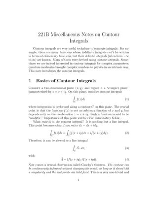
  • 5. A B 1 arctan − arctan a a a π 1 π π − − = = . a 2 2 a = lim A→∞ B→−∞ (20) On the other hand, this is what we would do with contour integrals. First of all, we regard this integral as a contour integral along the real axis on the complex plane. (We now view x as a complex parameter.) At the inifinity |x| → ∞, no matter at what angle, the integrand damps as 1/|x|2 . Therefore, even if we add a contour from +∞ going up in circle and come down at −∞, the additional piece can give correction suppressed by 1/|x| and hence vanishes. What it means is that we can regard the integral as a closed-contour integral along the real axis, going up at the infinity on the upper half plane, coming back to the real axis at −∞. On the other hand, the integrand can be rewritten as 1 1 = . x 2 + a2 (x + ia)(x − ia) (21) Therefore in the closed contour described above, the pole at x = +ia is encircled. The factor 1/(x + ia) corresponds to f (z) in Eq. (16). Then the result can be obtained immediately as C x2 dx = + a2 C 1/(x + ia) 1 π dx = 2πi = . x − ia ia + ia a (22) This result indeed agrees with the standard method. When we extended the contour at the infinity, we could have actually go down on the lower half plane. This defines another contour C that encircles the other pole at x = −ia. Do we obtain the same result this way, too? Let’s do it: dx 1/(x − ia) 1 π = dx = −2πi = . (23) x + ia −ia − ia a C x 2 + a2 C Here, we had to be careful about the fact that the contour C encircles the pole clockwise, that made the overall contribution of the residue come with the coefficient −2πi instead of 2πi. Now we see that contour integrals indeed work! 5
  • 6. x ia – ia Figure 1: Contour for the integrand 1/(x2 + a2 ). 3 More non-trivial cross-checks Now consider the following example1 ∞ dx . (24) −∞ cosh x The standard method is to find the indefinite integral, which is known to be x dx = 2 arctan tanh , (25) cosh x 2 which is easy to verify by differentiating it. Given this indefinite integral, the definite integral is simply ∞ −∞ dx x = 2 arctan tanh cosh x 2 ∞ = −∞ π π − − 2 2 = π. (26) We calculate this integral using a contour integral. The orignal integral is done along the real axis C1 on complex x plane. Now we add another section in the opposite direction parallel to the real axis but with the imaginary part π: C2 . Note that cosh(x + iπ) = 1 ex+iπ + e−(x+iπ) −ex − e−x = = − cosh x. 2 2 I thank Roni Harnik for this example. 6 (27)
  • 7. Therefore, the integral along C2 must be the same as that along C1 . Finally, we can close the contour at −∞ and ∞ because cosh x grows exponentially and hence 1/ cosh x is exponentially damped there. Then the closed contour integral, first along the real axis C1 , up to the imaginary part iπ at ∞, then back parallel to the real axis C2 , and down to the real axis at −∞, must give twice of the original integral we wanted. x iπ iπ/2 Figure 2: The integration countour for the integral 1/ cosh x. It can be smoothly deformed to that around the pole at x = iπ/2. 1 The poles of 1/ cosh x are all along the imaginary axis at x = i(n + 2 )π. In the closed contour integral, only the pole at x = iπ/2 is encircled counterclockwise. To identify the residue, we expand cosh x at x = iπ/2 as cosh i π +x 2 = cosh i π π + x sinh i + O(x )2 = 0 + ix + O(x )2 . 2 2 (28) Therefore, the contour integral reduces to that around the pole dx = cosh x 0 1 dx = 2πi = 2π. ix i (29) Because this is supposed to be twice as large as the original integral along the real axis, the wanted result is π. It agrees indeed with the conventional method. 7
  • 8. 4 New Integrals There are many integrals I cannot imagine doing without using contour integrals. Here is one simple example, ∞ −∞ eiqx dq. q 2 + a2 (30) We assume a > 0 without loss of generality. When x > 0, we can add an additional arc at the infinity on the upper half plane because that section gives an exponentially damped contribution. This makes the contour closed and it encirles the pole at q = ia. Hence the result is ∞ −∞ eiqx dq = q 2 + a2 ia e−ax e−ax eiqx dq = 2πi =π . (q + ia)(q − ia) 2ia a (31) On the other hand, when x < 0, the same added section is exponentially enhanced instead of damped, and we cannot add it. Instead, we add a section at the infinity on the lower half plane. Then the contour encircles the pole at q = −ia clockwise, and hence ∞ −∞ eiqx dq = − q 2 + a2 −ia eiqx eax eax dq = −2πi =π . (q + ia)(q − ia) −2ia a (32) Either way, the result can be summarized as πe−a|x| /a. This is actually the Yukawa-potential in one-dimension, or Green’s function for the equation 2 (∂x − a2 )G(x) = −2πδ(x). (33) This is easy to see from the integral expression, 2 (∂x − a2 ) ∞ −∞ eiqx dq = q 2 + a2 ∞ −∞ (−q 2 − a2 )eiqx dq q 2 + a2 ∞ = − eiqx dq −∞ = −2πδ(x). (34) The result of the contour integral can be verified to satisfy this equation, π 2 (∂x − a2 ) e−a|x| = ∂x (−π(sign x)e−a|x| ) − πae−a|x| a = πa(sign x)2 e−a|x| − 2πδ(x)e−a|x| − πae−a|x| = −2πδ(x). (35) 8
  • 9. Here we used +1 −1 ∂x |x| = sign x = x>0 , x<0 (36) (sign x)2 = 1, and ∂x sign x = 2δ(x). q ia – ia Figure 3: The contour for the integrand eiqx /(q 2 +a2 ) when x > 0. The added arc section on the upper half plane is exponentially damped and vanishes in the limit of taking the arc to infinity. When x < 0, an arc on the lower half plane is added instead. If we have only one pole instead of one, e.g., ∞ G(x) = −∞ eiqx dq, q − ia (37) the result is more interesting: it vanishes when k < 0 because the contour on the lower half plane does not encirle a pole. The result is therefore G(x) = 2πiθ(x)e−ax , (38) where θ(x) is the step function θ(x) = 1 0 9 x>0 x < 0. (39)
  • 10. As a limit, a → 0 gives just the step function with an exponential factor. This G(x) can also be viewed as a Green’s function for a differential equation. From the definition, ∞ (∂x + a)G(x) = −∞ (iq + a)eiqx dq = q − ia ∞ ieiqx dq = 2πiδ(x). (40) −∞ It is straightforward to check that our result G(x) = θ(x)e−ax satisifes the differential equation, noting ∂x θ(x) = δ(x). 5 Real-Life Examples Here are some real-life examples. 5.1 Three-dimensional Coulomb potential This is an example well-known to you. The scalar potential in electromagnetism satisfies the Poisson equation ∆φ = −4πρ, (41) where ρ is the charged density. (In MKSA system, the r.h.s. is −ρ/ 0 .) The standard way to solve this equation is to first solve the Green’s equation ∆G(x − x ) = δ(x − x ). (42) Once you have a solution “Green’s function,” the solution to the original equation is given simply by φ(x) = −4π dx G(x − x )ρ(x ). (43) The way to solve the Green’s equation is to use a Fourier transform, G(x) = dq ˜ G(q)eiq·x . 3 (2π) (44) Of course the delta function is a Fourier-transform of unity, δ(x) = dq iq·x e . (2π)3 10 (45)
  • 11. By substituting these expressions into the Green’s equation, we find ˜ − q 2 G(q) = 1. (46) ˜ Therefore, G(q) = 1/q 2 and hence dq −1 iq·x e . (2π)3 q 2 G(x) = (47) Now we go to spherical coordinates, q 2 dqd cos θdφ 1 iqr cos θ e . (2π)3 q2 G(x) = − (48) The integral over the azimuth is trivial: just a factor of 2π. Then the integral over cos θ can be done and we find ∞ G(x) = − 0 dq 1 eiqr − e−iqr . 2 iqr (2π) (49) Of course I can write the integrand in terms of sin qr, but let me keep it that way. The integration over q is from 0 to ∞, but the integrand is an even function of q, and we can extend it to the entire real axis with a factor of a half, 1 1 ∞ eiqr − e−iqr dq . (50) G(x) = − 2 8π i r −∞ q The integrand is regular at q = 0 because of the numerator. Therefore, we can safely regard it as a limit of the integral ∞ dq −∞ eiqr − e−iqr . q+i (51) There is now a pole at q = −i . Let us assume > 0 for the moment. Note that r > 0. Therefore, for the piece eiqr , we can extend the contour on the upper half plane. This contour does not encirle the pole. On the other hand, for the piece e−iqr , we can extend the contour on the lower half plane, and pick up the pole. Therefore, ∞ dq −∞ eiqr − e−iqr = −2πi(−e− r ). q+i 11 (52)
  • 12. Suppose now that < 0. In this case the opposite happens. We now get the contribution from the pole for the piece eiqr , and we find ∞ dq −∞ eiqr − e−iqr = 2πi(e r ). q+i (53) Either way, we find the same result 2πi in the limit → 0. Therefore, G(x) = − 1 1 1 1 2πi = − . 8π 2 i r 4π r (54) This is nothing but the Coulomb potential. A by-product of this calculation is the formula ∞ dq −∞ sin qr = π, q (55) independent of r. The indefinite integral is called Sine-Integral function Si (x), x sin t dt, (56) Si (x) = t 0 which cannot be expressed in terms of elementary functions. What we learned from the contour integral is Si (∞) = π/2. 5.2 Lippmann–Schwinger Kernel In the Lippmann–Schwinger equation, we need the operator 1/(E − H0 + i ). In the position representation, it defines a Green’s function G(x − x ) = lim x| →+0 1 |x E − H0 + i (57) which satisfies the equation E+ h2 ∆ ¯ G(x − x ) = 2m h2 ∆ ¯ 1 x| |x 2m E − H0 + i p2 1 = x| E − |x 2m E − H0 + i = x|x = δ(x − x ). E+ 12 (58)
  • 13. Here, the one-sided limit → +0 is understood but not written explicitly. By inserting the complete set of states in the momentum representation, and using the fact that H0 is diagonal in the momentum space, we find G(x, x ) = dp x|p 1 E− p2 /2m +i p|x = h h eix·p/¯ 1 e−ix ·p/¯ dp (2π¯ )3/2 E − p2 /2m + i (2π¯ )3/2 h h = dp h 1 ei(x−x )·p/¯ . (2π¯ )3 E − p2 /2m + i h (59) There are many ways to do this integration. One way is to use polar coordinates for p defining the polar angle relative to the direction of r = x − x such that h eipr cos θ/¯ 1 3 E − p2 /2m + i (2π¯ ) h 0 −1 0 ipr/¯ h −ipr/¯ h ∞ 2π e −e 1 = p2 dp (2π¯ )3 0 h ipr/¯ h E − p2 /2m + i h ∞ eipr/¯ −2m 1 pdp = 2 −∞ 2 − 2mE − i (2π¯ ) h ir p h 1 2mi ∞ peipr/¯ √ √ = dp . (60) (2π¯ )2 r −∞ (p − 2mE − i )(p + 2mE + i ) h ∞ G(r) = p2 dp 2π 1 dφ d cos θ h Because of the numerator eipr/¯ , we can extend the integration contour to go along the real axis and come back at the infinity on the upper half plane. √ Then the contour integral picks up only the pole at p = 2mE +i = hk +i , ¯ and we find 1 2mi hkeikr ¯ 2πi 2 r (2π¯ ) h 2¯ k h ikr 2m e = − 2 . h 4πr ¯ G(r) = (61) This Green’s function describes the wave propagating outwards from a point source. If we had approached the pole from the opposite side, we had gotten a different result. The contour on the upper half plane would pick the pole at 13
  • 14. √ p = − 2mE = −¯ k instead, and we find h −¯ ke−ikr h 1 2mi 2πi 2 r (2π¯ ) h −2¯ k h −ikr 2m e = − 2 . h 4πr ¯ G(r) = (62) This Green’s function describes the wave propagating towards a point sink. It is hard to imagine setting up an initial condition so that the wave would converge exactly to a point. Because of this reason, this Green’s function is not used in the scattering problem. 6 Principal Value Integral Here, we introduce the following identity 1 1 =P x±i x iπδ(x). (63) When one encounters an integral of the type b −a f (x) dx x (64) along the real axis, it is ill-defined at x = 0 unless f (x) = 0. It is a mild logarithmic singularity, but it is a singularity nonetheless. One way to define such an integral is as a limit of lim →+0 f (x) dx. x±i (65) It turns out that the result depends on which way you avoid the singularity (choice of the sign of i in the denominator). It is always assumed that > 0 and hence the one-sided limit → +0. Let us first study the limit lim →+0 f (x) dx. x−i (66) In this case, the pole is at x = +i and above the real axis. Therefore, the limit → 0 defines the integral along the contour shown in the figure Fig. 4. 14
  • 15. x Figure 4: The integral 1/(x − i ) defined by the limit → +0. The integral consists of three pieces. First, the integral along the real axis, except that the singularity is avoided symmetrically around the origin. In other words, there is an integral −ε b + dx −a ε f (x) . x (67) By taking ε infinitesimally small, the singularity cancels between the contributions from the left and right of the pole. This way, the integral is made well-defined. This contribution is called the principal value integral , and denoted by b f (x) −ε b f (x) P dx = + dx . (68) x −a x −a ε Second, there is an arc below the pole. By taking the radius of the circle infinitesimally small, we can take f (x) to be constant f (0), and the integral along the semi-circle is a half of that from a closed contour integral. Therefore, the additional piece is ε iπf (0) = iπδ(x)f (x)dx. (69) −ε The whole integral then is given by the sum of two pieces, b lim →0 −a f (x) dx = P x−i b −a f (x) dx + x b iπδ(x)f (x)dx. (70) −a To express this identity, we can write 1 1 = P + iπδ(x), x−i x 15 (71)
  • 16. as long as it is understood that P is the principal value integral and the entire right-hand side is inside an integral. The case with the opposite way to avoid the pole 1/(x + i ) is done very similarly, and we find 1 1 = P − iπδ(x). (72) x+i x The source of the minus sign in front of the second term is because the semi-circle around the pole goes clockwise in this case. We can test these formulae with a simple example, ∞ dx −∞ cos x . x−i (73) Writing cos x = (eix + e−ix )/2, the first term allows us to add a semi-circle on the upper half plane, while the second term on the lower half plane. Because the pole is at x = +i , only the semi-circle on the upper half plane encirles the pole. Therefore, ∞ dx −∞ cos x 1 = 2πi = iπ. x−i 2 (74) On the other hand, the principal value intergral is ∞ P dx −∞ cos x = 0. x (75) This follows from the definition ∞ P dx −∞ cos x = lim →0 x − dx −∞ cos x + x ∞ dx cos x x (76) together with the change of the variable x → −x in the first term, ∞ = lim − dx →0 cos x + x ∞ dx cos x = 0. x (77) It is crucial that the principal value prescription is symmetric around the pole. Finally, ∞ dx cos xiπδ(x) = iπ. (78) −∞ Putting Eqs. (74,77,78) together, the formula Eq. (71) indeed holds. 16
  • 17. Another way to look at the principal value integral is by combining Eqs. (71,72), 1 1 1 1 + . (79) P = x 2 x−i x+i The two terms in the r.h.s. avoid the pole from above and below. Therefore, you can also express it as b P dx a 1 f (x) = lim x 2 →0 b−i dx a−i f (x) + x b+i dx a+i f (x) , x (80) as shown graphically in Fig. 5. x Figure 5: The principal value integral is the same as the average of integrals just above and just below the pole. 7 Crazy Examples Now equipped with contour integrals and principal value integrals, we can prove some crazy examples I found in math books. For example, ∞ π sinh a sin ax 1 = if |a| < |b|. (81) dx sin bx 1 + x2 2 sinh b 0 This looks really crazy; how come is the integral of an oscillating function given in terms of hyperbolic functions? First of all, the integrand has many poles along the real axis, x = nπ/b. The prescription employed in math books is often the principal value prescription. Using the idea in Fig. 5, we first rewrite the integral as ∞+i ∞−i 1 sin ax 1 sin ax 1 = lim dx + dx . (82) 2 2 →0 sin bx 1 + x sin bx 1 + x2 − Then we change the variable from x to −x in the second term, ∞+i 1 sin ax 1 sin ax 1 = lim dx + dx 2 2 →0 sin bx 1 + x sin bx 1 + x2 −∞+i ∞+i 1 sin ax 1 = lim dx . (83) →0 −∞+i 2 sin bx 1 + x2 17
  • 18. The integration is above the real axis. Now the trick is to use the pole at x = +i. Because of the assumption |a| < |b|, the behavior of sin ax/ sin bx on the infinite semi-circle on the upper half plane is (for example when both a, b are positive), eiax − e−iax sin ax e−iax = ibx ∼ −ibx = e−i(a−b)x → 0. sin bx e − e−ibx e (84) Cases with other signs of a, b can also be seen easily and sin ax/ sin bx → 0. Therefore, we can add the inifinite semi-circle on the upper half plane to the integration contour, which closes the contour. The only pole inside the contour is at x = +i, and the by-now-standard steps lead to the result sin ia 1 π sinh a 1 lim 2πi = . 2 →0 sin ib 2i 2 sinh b Exactly the same method proves another formula = ∞ dx 0 sin ax x π sinh a =− 2 cos bx 1 + x 2 cosh b if |a| < |b|. (85) (86) The next one can be done with an indefinite integral, but is much easier with a contour integral: 2π 0 dx 2π = 1 − 2a cos x + a2 |1 − a2 | (a = ±1). (87) We assume a > 0 for the discussions below, but the case a < 0 can be done the same way. Along the real axis, 1 − 2a cos x +a2 = (1 − a)2 +2a(1− cos x) = (1− a)2 + 4a sin2 x > 0. However, along the imaginary axis x = iχ, 1 − 2a cos x + a2 = 2 2 1 − 2a cosh χ + a2 = 0 at χ = cosh−1 1+a . Therefore there is a pole along 2a the imaginary axis. Let us first shift the integration region to [−π, π] using the periodicity of cos x. Then further consider a rectangle as shown in Fig. 6. We will send the top side all the way to infinite in the end. The main point is that left and right sides cancel due to the periodicity in cos x. Moreover, the integral along the top side goes to zero in the limit because cos x = cosh χ → ∞. Therefore, the integration along the real axis (the bottom side) is the same as the contour integral along the rectangle. Then the contour integral encircles the pole at 2 x0 = iχ0 = i cosh−1 1+a , where 2a 1 − 2a cos x + a2 = 0 + (x − x0 )2ai sinh χ0 + O(x − x0 )2 . 18 (88)
  • 19. The integral is easily done as 2π 0 dx 1 . = 2πi 2 1 − 2a cos x + a 2a sin x0 (89) 2 The rest is to rewrite sin x0 . Because cosh χ0 = 1+a , sinh2 χ0 = cosh2 χ0 − 2a |1−a2 | (1−a2 )2 1 = 4a2 , and hence sinh χ0 = 2a . Therefore, we find 2π 0 dx 2π 1 = . = 2πi 2 1 − 2a cos x + a 2ai sinh χ0 |1 − a2 | x −π π Figure 6: The integration contour to study Eq. (87). 19 (90)