Hidden Markov Models Explained

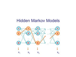
Hidden Markov Models
1
2
K
…
1
2
K
…
1
2
K
…
…
…
…
1
2
K
…
x1 x2 x3 xK
2
1
K
2

CS262 Lecture 6, Win06, Batzoglou
Viterbi, Forward, Backward
VITERBI
Initialization:
V0(0) = 1
Vk(0) = 0, for all k > 0
Iteration:
Vl(i) = el(xi) maxk Vk(i-1) akl
Termination:
P(x, π*) = maxk Vk(N)
FORWARD
Initialization:
f0(0) = 1
fk(0) = 0, for all k > 0
Iteration:
fl(i) = el(xi) Σk fk(i-1) akl
Termination:
P(x) = Σk fk(N) ak0
BACKWARD
Initialization:
bk(N) = ak0, for all k
Iteration:
bl(i) = Σk el(xi+1) akl bk(i+1)
Termination:
P(x) = Σk a0k ek(x1) bk(1)

A+ C+ G+ T+
A- C- G- T-
A modeling Example
CpG islands in DNA
sequences

Methylation & Silencing
• One way cells differentiate is
methylation
 Addition of CH3in C-nucleotides
 Silences genes in region
• CG (denoted CpG) often
mutates to TG, when methylated
• In each cell, one copy of X is
silenced, methylation plays role
• Methylation is inherited during
cell division

Example: CpG Islands
CpG nucleotides in the genome are frequently methylated
(Write CpG not to confuse with CG base pair)
C → methyl-C → T
Methylation often suppressed around genes, promoters
→ CpG islands

Example: CpG Islands
• In CpG islands,
 CG is more frequent
 Other pairs (AA, AG, AT…) have different frequencies
Question: Detect CpG islands computationally

A model of CpG Islands – (1)
Architecture
A+ C+ G+ T+
A- C- G- T-
CpG Island
Not CpG Island

Transitions
How do we estimate parameters of the model?
Emission probabilities: 1/0
1. Transition probabilities within CpG islands
Established from known CpG islands
(Training Set)
2. Transition probabilities within other regions
Established from known non-CpG islands
(Training Set)
Note: these transitions out of each state add
up to one—no room for transitions
between (+) and (-) states
+ A C G T
A .180 .274 .426 .120
C .171 .368 .274 .188
G .161 .339 .375 .125
T .079 .355 .384 .182
- A C G T
A .300 .205 .285 .210
C .233 .298 .078 .302
G .248 .246 .298 .208
T .177 .239 .292 .292
= 1
= 1
= 1
= 1
= 1
= 1
= 1
= 1

Log Likehoods—
Telling “Prediction” from “Random”
A C G T
A -0.740 +0.419 +0.580 -0.803
C -0.913 +0.302 +1.812 -0.685
G -0.624 +0.461 +0.331 -0.730
T -1.169 +0.573 +0.393 -0.679
Another way to see effects of
transitions:
Log likelihoods
L(u, v) = log[ P(uv | + ) / P(uv | -) ]
Given a region x = x1…xN
A quick-&-dirty way to decide
whether entire x is CpG
P(x is CpG) > P(x is not CpG) ⇒
Σi L(xi, xi+1) > 0

Transitions
• What about transitions between (+) and (-) states?
• They affect
 Avg. length of CpG island
 Avg. separation between two CpG islands
X Y
1-p
1-q
p q
Length distribution of region X:
P[lX = 1] = 1-p
P[lX = 2] = p(1-p)
…
P[lX= k] = pk-1
(1-p)
E[lX] = 1/(1-p)
Geometric distribution, with mean 1/
(1-p)

A+ C+ G+ T+
A- C- G- T-
1–p
Transitions
Right now, aA+A+ + aA+C+ + aA+G+ + aA+T+ = 1
We need to adjust aij so as to allow transitions between (+) and (-) states
Say we want with probability p++ to stay within CpG, p-- to stay within non-CpG
1. Let’s adjust all probs by that factor: example, let aA+G+ ← p++ × aA+G+
2. Now, let’s calculate probs between (+) and (-) states
1. Total prob aA+S where S is a (-) state, is (1 – p++)
2. Let qA-, qC-, qG-, qT- be the proportions of A, C, G, and T within non-CpG states in training set
3. Then, let aA+A- = (1 – p++) × qA-; aA+C- = (1 – p++) × qC-; …
4. Do the same for (-) to (+) states
3. OK, but how do we estimate p++ and p--?
1. Estimate average length of a CpG island: l+ = 1/(1-p) ⇒ p = 1 – 1/l+
2. Do the same for length between two CpG islands, l

Applications of the model
Given a DNA region x,
The Viterbi algorithm predicts locations of CpG islands
Given a nucleotide xi, (say xi = A)
The Viterbi parse tells whether xi is in a CpG island in the most likely
general scenario
The Forward/Backward algorithms can calculate
P(xi is in CpG island) = P(πi = A+
| x)
Posterior Decoding can assign locally optimal predictions of CpG islands
π^
i = argmaxk P(πi = k | x)

What if a new genome comes?
• We just sequenced the porcupine genome
• We know CpG islands play the same role in
this genome
• However, we have no known CpG islands for
porcupines
• We suspect the frequency and characteristics
of CpG islands are quite different in
porcupines
How do we adjust the parameters in our model?
LEARNING

Problem 3: Learning
Re-estimate the parameters of the
model based on training data

Two learning scenarios
1. Estimation when the “right answer” is known
Examples:
GIVEN: a genomic region x = x1…x1,000,000 where we have good
(experimental) annotations of the CpG islands
GIVEN: the casino player allows us to observe him one evening,
as he changes dice and produces 10,000 rolls
2. Estimation when the “right answer” is unknown
Examples:
GIVEN: the porcupine genome; we don’t know how frequent are the
CpG islands there, neither do we know their composition
GIVEN: 10,000 rolls of the casino player, but we don’t see when he
changes dice
QUESTION: Update the parameters θ of the model to maximize P(x|θ)

1. When the right answer is known
Given x = x1…xN
for which the true π = π1…πN is known,
Define:
Akl = # times k→l transition occurs in π
Ek(b) = # times state k in π emits b in x
We can show that the maximum likelihood parameters θ (maximize P(x|θ)) are:
Akl Ek(b)
akl = ––––– ek(b) = –––––––
Σi Aki Σc Ek(c)

1. When the right answer is known
Intuition: When we know the underlying states,
Best estimate is the average frequency of
transitions & emissions that occur in the training data
Drawback:
Given little data, there may be overfitting:
P(x|θ) is maximized, but θ is unreasonable
0 probabilities – VERY BAD
Example:
Given 10 casino rolls, we observe
x = 2, 1, 5, 6, 1, 2, 3, 6, 2, 3
π = F, F, F, F, F, F, F, F, F, F
Then:
aFF = 1; aFL = 0
eF(1) = eF(3) = .2;
eF(2) = .3; eF(4) = 0; eF(5) = eF(6) = .1

Pseudocounts
Solution for small training sets:
Add pseudocounts
Akl = # times k→l transition occurs in π + rkl
Ek(b) = # times state k in π emits b in x + rk(b)
rkl, rk(b) are pseudocounts representing our prior belief
Larger pseudocounts ⇒ Strong priof belief
Small pseudocounts (ε < 1): just to avoid 0 probabilities

Pseudocounts
Example: dishonest casino
We will observe player for one day, 600 rolls
Reasonable pseudocounts:
r0F = r0L = rF0 = rL0 = 1;
rFL = rLF = rFF = rLL = 1;
rF(1) = rF(2) = … = rF(6) = 20 (strong belief fair is fair)
rL(1) = rL(2) = … = rL(6) = 5 (wait and see for loaded)
Above #s pretty arbitrary – assigning priors is an art

2. When the right answer is unknown
We don’t know the true Akl, Ek(b)
Idea:
• We estimate our “best guess” on what Akl, Ek(b) are
• We update the parameters of the model, based on our guess
• We repeat

2. When the right answer is unknown
Starting with our best guess of a model M, parameters θ:
Given x = x1…xN
for which the true π = π1…πN is unknown,
We can get to a provably more likely parameter set θ
i.e., θ that increases the probability P(x | θ)
Principle: EXPECTATION MAXIMIZATION
1. Estimate Akl, Ek(b) in the training data
2. Update θ according to Akl, Ek(b)
3. Repeat 1 & 2, until convergence

Estimating new parameters
To estimate Akl: (assume | θCURRENT, in all formulas below)
At each position i of sequence x, find probability transition k→l is used:
P(πi = k, πi+1 = l | x) =
[1/P(x)] × P(πi = k, πi+1 = l, x1…xN) = Q/P(x)
where Q = P(x1…xi, πi = k, πi+1 = l, xi+1…xN) =
= P(πi+1 = l, xi+1…xN | πi = k) P(x1…xi, πi = k) =
= P(πi+1 = l, xi+1xi+2…xN | πi = k) fk(i) =
= P(xi+2…xN | πi+1 = l) P(xi+1 | πi+1 = l) P(πi+1 = l | πi = k) fk(i) =
= bl(i+1) el(xi+1) akl fk(i)
fk(i) akl el(xi+1) bl(i+1)
So: P(πi = k, πi+1 = l | x, θ) = ––––––––––––––––––
P(x | θCURRENT)

Estimating new parameters
• So, Akl is the E[# times transition k→l, given current θ]
fk(i) akl el(xi+1) bl(i+1)
Akl = Σi P(πi = k, πi+1 = l | x, θ) = Σi –––––––––––––––––
P(x | θ)
• Similarly,
Ek(b) = [1/P(x | θ)]Σ{i | xi = b} fk(i) bk(i)
k l
xi+1
akl
el(xi+1)
bl(i+1)fk(i)
x1………xi-1
xi+2………xN
xi

The Baum-Welch Algorithm
Initialization:
Pick the best-guess for model parameters
(or arbitrary)
Iteration:
1. Forward
2. Backward
3. Calculate Akl, Ek(b), given θCURRENT
4. Calculate new model parameters θNEW : akl, ek(b)
5. Calculate new log-likelihood P(x | θNEW)
GUARANTEED TO BE HIGHER BY EXPECTATION-MAXIMIZATION
Until P(x | θ) does not change much

The Baum-Welch Algorithm
Time Complexity:
# iterations × O(K2
N)
• Guaranteed to increase the log likelihood P(x | θ)
• Not guaranteed to find globally best parameters
Converges to local optimum, depending on initial
conditions
• Too many parameters / too large model: Overtraining

Alternative: Viterbi Training
Initialization: Same
Iteration:
1. Perform Viterbi, to find π*
2. Calculate Akl, Ek(b) according to π*
+ pseudocounts
3. Calculate the new parameters akl, ek(b)
Until convergence
Notes:
 Not guaranteed to increase P(x | θ)
 Guaranteed to increase P(x, | θ, π*
)
 In general, worse performance than Baum-Welch

Variants of HMMs

Higher-order HMMs
• How do we model “memory” larger than one time point?
• P(πi+1 = l | πi = k) akl
• P(πi+1 = l | πi = k, πi -1 = j) ajkl
• …
• A second order HMM with K states is equivalent to a first order HMM
with K2
states
state H state T
aHT(prev = H)
aHT(prev = T)
aTH(prev = H)
aTH(prev = T)
state HH state HT
state TH state TT
aHHT
aTTH
aHTTaTHH
aTHT
aHTH

Modeling the Duration of States
Length distribution of region X:
E[lX] = 1/(1-p)
• Geometric distribution, with mean 1/(1-p)
This is a significant disadvantage of HMMs
Several solutions exist for modeling different length distributions
X Y
1-p
1-q
p q

Example: exon lengths in genes

Solution 1: Chain several states
X Y
1-p
1-q
p
qXX
Disadvantage: Still very inflexible
lX = C + geometric with mean 1/(1-p)

Solution 2: Negative binomial distribution
Duration in X: m turns, where
 During first m – 1 turns, exactly n – 1 arrows to next state are followed
 During mth
turn, an arrow to next state is followed
m – 1 m – 1
P(lX = m) = n – 1 (1 – p)n-1+1
p(m-1)-(n-1)
= n – 1 (1 – p)n
pm-n
X(n)
p
X(2)X(1)
p
1 – p1 – p
p
…… Y
1 – p

Example: genes in prokaryotes
• EasyGene:
Prokaryotic
gene-finder
Larsen TS, Krogh A
• Negative binomial with n = 3

Solution 3: Duration modeling
Upon entering a state:
1. Choose duration d, according to probability distribution
2. Generate d letters according to emission probs
3. Take a transition to next state according to transition probs
Disadvantage: Increase in complexity:
Time: O(D)
Space: O(1)
where D = maximum duration of state
F d<Df xi…xi+d-1
Pf
Warning, Rabiner’s
tutorial claims O(D2)
& O(D) increases

Viterbi with duration modeling
Recall original iteration:
VF(i) = maxk Vk(i – 1) akl × eF(xi)
New iteration:
VF(i) = maxk maxd=1…Df Vk(i – d) × Pf(d) × akF × Πj=i-d+1…ieF(xj)
F L
transitions
emissions
d<Df
xi…xi + d – 1
emissions
d<Dl
xj…xj + d – 1
Pf Pl
Precompute
cumulative
values

Hidden Markov Models Explained

Empfohlen

Empfohlen

Weitere ähnliche Inhalte

Was ist angesagt?

Was ist angesagt? (20)

Ähnlich wie Hidden Markov Models Explained

Ähnlich wie Hidden Markov Models Explained (20)

Mehr von BioinformaticsInstitute

Mehr von BioinformaticsInstitute (20)

Kürzlich hochgeladen

Kürzlich hochgeladen (20)

Hidden Markov Models Explained

Hinweis der Redaktion