SlideShare a Scribd company logo
1 of 8
Download to read offline
ESTADÍSTICA GENERAL Y APLICADA
FORMULARIO
Semana 1:
Tabla de frecuencias por intervalos
Paso 1: Calcule el rango (R):
𝑹 = 𝑿𝒎𝒂𝒙 − 𝑿𝒎𝒊𝒏
Paso 2: Calcule el número de clases o intervalos (k) utilizando la regla de Sturges:
𝒌 = 𝟏 + 𝟑. 𝟑 𝒍𝒐𝒈 𝒏
Paso 3: Calcule la amplitud del intervalo de clase (c):
𝒄 =
𝑹
𝒌
Semana 2:
Medidas de tendencia central (datos no agrupados)
Media aritmética
𝑿
̅ =
∑ 𝑿𝒊
𝒏
Propiedades de la media aritmética
Nueva Variable Nueva Media
𝒚𝒊 = 𝒙𝒊 ± 𝒃 𝒚
̅ = 𝒙
̅ ± 𝒃
𝒚𝒊 = 𝒄 𝒙𝒊 𝒚
̅ = 𝒄𝒙
̅
𝒚𝒊 = 𝒄𝒙𝒊 ± 𝒃 𝒚
̅ = 𝒄𝒙
̅ ± 𝒃
Mediana
Impar: 𝑴𝒆 = 𝒙(
𝒏+𝟏
𝟐
)
Par: 𝑴𝒆 =
𝒙
(
𝒏
𝟐
)
+𝒙
(
𝒏
𝟐
+𝟏)
𝟐
Moda (Dato más frecuente)
Medidas de tendencia no central (datos no agrupados)
Cálculo de percentiles
1. Ordenar los datos en forma ascendente.
2. Hallar la posición (j) del percentil (Pk) a partir de la siguiente expresión:
𝒋 =
𝒌(𝒏 + 𝟏)
𝟏𝟎𝟎
3. Ubicar el percentil en la posición hallada si “j” es un número entero; caso contrario, el
percentil se calcula con la siguiente fórmula:
𝑷𝒌 = 𝑳𝒊 + 𝒅𝒆𝒄 × (𝑳𝒅 − 𝑳𝒊)
Semana 3:
Medidas de variabilidad
 Rango: 𝑹 = 𝑿𝒎𝒂𝒙 − 𝑿𝒎𝒊𝒏
 Rango Intercuartilico: 𝑹𝑰 = 𝑸𝟑 − 𝑸𝟏
 Varianza: 𝒔𝟐
=
∑ 𝑿𝒊
𝟐
−𝒏𝑿
̅𝟐
𝒏
𝒊=𝟏
𝒏−𝟏
 Desviación Estándar: 𝒔 = √𝒔𝟐
 Coeficiente de Variación 𝑪𝑽 =
𝑺
𝑿
̅ × 𝟏𝟎𝟎
Propiedades de la Varianza
Nueva Variable Nueva Media Nueva varianza Nueva desviación estándar
𝒚𝒊 = 𝒙𝒊 ± 𝒃 𝒚
̅ = 𝒙
̅ ± 𝒃 𝒔𝒚
𝟐
= 𝒔𝒙
𝟐 𝒔𝒚 = 𝒔𝒙
𝒚𝒊 = 𝒄 𝒙𝒊 𝒚
̅ = 𝒄𝒙
̅ 𝒔𝒚
𝟐
= 𝒄𝟐
𝒔𝒙
𝟐
𝒔𝒚 = 𝒄𝒔𝒙
𝒚𝒊 = 𝒄𝒙𝒊 ± 𝒃 𝒚
̅ = 𝒄𝒙
̅ ± 𝒃 𝒔𝒚
𝟐
= 𝒄𝟐
𝒔𝒙
𝟐
𝒔𝒚 = 𝒄𝒔𝒙
Medidas de Forma
 Coeficiente de Asimetría
𝑨𝒌 =
𝟑(𝑿
̅ − 𝑴𝒆)
𝑺
Medidas de Concentración
 Coeficiente de Curtosis.
𝑲𝒖 =
𝑸𝟑 − 𝑸𝟏
𝟐(𝑷𝟗𝟎 − 𝑷𝟏𝟎)
=
𝑷𝟕𝟓 − 𝑷𝟐𝟓
𝟐(𝑷𝟗𝟎 − 𝑷𝟏𝟎)
Semana 4:
 Probabilidad
 Experimento aleatorio
 Espacio muestral: (Ω)
 Eventos: A, B, C…
 Operaciones entre eventos.
Unión: 𝑨 ∪ 𝑩
Intersección: 𝑨 ∩ 𝑩
Eventos mutuamente excluyentes 𝑨 ∩ 𝑩 = ∅
 Probabilidad de un evento:
𝑷(𝑨) =
𝒏 (𝑨)
𝒏(𝜴)
 Probabilidad condicional
𝑷(𝑨/𝑩) =
𝑷(𝑨 ∩ 𝑩)
𝑷(𝑩)
 Principio de adición para 2 eventos
𝑷(𝑨 ∪ 𝑩) = 𝑷(𝑨) + 𝑷(𝑩) − 𝑷(𝑨 ∩ 𝑩)
Semana 5:
 Principio de multiplicación para n eventos
𝑷(𝑨𝟏 ∩ 𝑨𝟐 ∩ … ∩ 𝑨𝒏) = 𝑷(𝑨𝟏) 𝑷(𝑨𝟐/𝑨𝟏) … 𝑷(𝑨𝒏/𝑨𝟏 ∩ … ∩ 𝑨𝒏−𝟏)
 Eventos independientes para 2 eventos
𝑷(𝑨/𝑩) = 𝑷(𝑨) 𝑷(𝑨 ∩ 𝑩) = 𝑷(𝑨) × 𝑷(𝑩)
 Teorema de probabilidad total
𝑷(𝑨) = 𝑷(𝑨𝟏) × 𝑷(𝑨/𝑨𝟏) + 𝑷(𝑨𝟐) × 𝑷(𝑨/𝑨𝟐) + ⋯ + 𝑷(𝑨𝒏) × 𝑷(𝑨/𝑨𝒏)
 Teorema de Bayes
𝑷(𝑨𝒊/ 𝑨) =
𝑷(𝑨𝒊 ∩ 𝑨)
𝑷(𝑨)
𝑷(𝑨𝒊/ 𝑨) =
𝑷(𝑨𝒊) × 𝑷(𝑨/𝑨𝒊)
𝑷(𝑨𝟏) × 𝑷(𝑨/𝑨𝟏) + 𝑷(𝑨𝟐) × 𝑷(𝑨/𝑨𝟐) + ⋯ + 𝑷(𝑨𝒏) × 𝑷(𝑨/𝑨𝒏)
;  𝒊
Semana 6:
Distribución Binomial
 Función de probabilidad de la distribución Binomial.
𝑷(𝑿 = 𝒙) = ∁𝒙
𝒏
𝒑𝒙(𝟏 − 𝒑)𝒏−𝒙
Medidas de resumen.
Esperanza Matemática 𝑬(𝑿) = 𝒏 𝒑
Varianza 𝑽(𝑿) = 𝒏 𝒑(𝟏 − 𝒑)
Distribución Poisson
 Función de probabilidad de la distribución Poisson.
𝑷(𝑿 = 𝒙) = 𝒆−𝝀
×
𝝀𝒙
𝒙!
Medidas de resumen.
Esperanza Matemática 𝑬(𝑿) = 𝝀
Varianza 𝑽(𝑿) = 𝝀
Semana 7:
Distribución normal
 Estandarización
𝒁 =
𝑿 − 𝝁
𝝈
ESTADISTICA APLICADA
Semana 1:
Estimación por intervalo para la media o promedio poblacional 𝝁:
 Caso I: Cuando σ2
es conocido:
𝑰𝑪(𝝁) = 〈𝒙
̅ ± 𝒁𝟏−𝜶 𝟐
⁄
𝝈
√𝒏
〉
 Caso II: Cuando σ2
es desconocido (n≤ 30)
𝑰𝑪(𝝁) = 〈𝒙
̅ ± 𝒕𝟏−𝜶 𝟐
⁄ ;𝒏−𝟏
𝑺
√𝒏
〉
 Caso III: Cuando σ2
es desconocido (n> 30)
𝑰𝑪(𝝁) = 〈𝒙
̅ ± 𝒛𝟏−𝜶 𝟐
⁄
𝑺
√𝒏
〉
Estimación por intervalo para la proporción poblacional 𝝅:
𝑰𝑪(𝝅) = 𝒑 ± 𝒁𝟏−𝜶 𝟐
⁄ √
𝒑(𝟏 − 𝒑)
𝒏
Estimación por intervalo para la varianza poblacional 𝝈𝟐
:
(𝒏 − 𝟏)𝒔𝟐
𝝌𝟏−𝜶 𝟐
⁄ ;𝒏−𝟏
𝟐
≤ 𝝈𝟐
≤
(𝒏 − 𝟏)𝒔𝟐
𝝌𝜶 𝟐
⁄ ;𝒏−𝟏
𝟐
Tamaño de muestra
Media
𝒏𝟎 =
𝒛𝟏−𝜶 𝟐
⁄
𝟐
× 𝝈𝟐
𝜺𝟐
Proporción:
𝒏𝟎 =
𝒛𝟏−𝜶 𝟐
⁄
𝟐
𝒑(𝟏 − 𝒑)
𝜺𝟐
Factor de corrección si se conoce la población
𝒏 =
𝒏𝟎
𝟏 +
𝒏𝟎
𝑵
Semana 2:
Intervalo de confianza para el cociente de varianzas (𝝈𝟏
𝟐
𝝈𝟐
𝟐
⁄ )
〈
𝒔𝟏
𝟐
𝒔𝟐
𝟐
×
𝟏
𝑭𝜶 𝟐
⁄ , 𝒏𝟏−𝟏; 𝒏𝟐−𝟏
≤
𝝈𝟏
𝟐
𝝈𝟐
𝟐
≤
𝒔𝟏
𝟐
𝒔𝟐
𝟐
× 𝑭𝜶 𝟐
⁄ , 𝒏𝟐−𝟏; 𝒏𝟏−𝟏〉
Intervalo de confianza para las diferencias de medias poblacionales (𝝁𝟏 − 𝝁𝟐)
 Caso 1: Cuando las varianzas poblacionales son conocidas
𝑰𝑪(𝝁𝟏 − 𝝁𝟐) : (𝒙
̅ − 𝒚
̅) ± 𝒛𝟏−𝜶 𝟐
⁄ √
𝝈𝟏
𝟐
𝒏𝟏
+
𝝈𝟐
𝟐
𝒏𝟐
 Caso 2: Cuando las varianzas poblacionales son desconocidas pero homogéneas
𝑰𝑪(𝝁𝟏 − 𝝁𝟐) : (𝒙
̅ − 𝒚
̅) ± 𝒕𝟏−𝜶 𝟐
⁄ ;𝒏𝟏+𝒏𝟐−𝟐
√(
(𝒏𝟏 − 𝟏)𝒔𝟏
𝟐
+ (𝒏𝟐 − 𝟏)𝒔𝟐
𝟐
𝒏𝟏 + 𝒏𝟐 − 𝟐
) (
𝟏
𝒏𝟏
+
𝟏
𝒏𝟐
)
 Caso 3: Cuando las varianzas poblacionales son desconocidas, pero no homogéneas
𝑰𝑪(𝝁𝟏 − 𝝁𝟐) : (𝒙
̅ − 𝒚
̅) ± (𝒕𝟏−𝜶 𝟐
⁄ ; 𝒈 ) √
𝒔𝟏
𝟐
𝒏𝟏
+
𝒔𝟐
𝟐
𝒏𝟐
Grados de libertad
𝒈 =
[
𝒔𝟏
𝟐
𝒏𝟏
+
𝒔𝟐
𝟐
𝒏𝟐
]
𝟐
[
𝒔𝟏
𝟐
𝒏𝟏
]
𝟐
𝒏𝟏 + 𝟏 +
[
𝒔𝟐
𝟐
𝒏𝟐
]
𝟐
𝒏𝟐 + 𝟏
− 𝟐
Intervalo de confianza para la diferencia de 2 proporciones poblacionales (𝝅𝟏 − 𝝅𝟐)
𝑰𝑪(𝝅𝟏 − 𝝅𝟐) : (𝒑 𝟏
− 𝒑𝟐) ± 𝒛𝟏−𝜶 𝟐
⁄ √
𝒑𝟏(𝟏 − 𝒑𝟏)
𝒏𝟏
+
𝒑𝟐(𝟏 − 𝒑𝟐)
𝒏𝟐
Semana 3:
PROCEDIMIENTO PARA REALIZAR UNA PRUEBA DE HIPÓTESIS
Paso 1 (Plantee las hipótesis de prueba)
Paso 2 (Establezca el nivel de significancia) α
Paso 3 (Calcule el valor del estadístico de prueba)
La decisión de aceptar o rechazar la hipótesis nula, se hace en base al valor del estadístico de
contraste (estadístico de prueba), este valor se obtiene con los datos de la muestra.
Paso 4 Regla de decisión
La región de rechazo, también conocida como región crítica, se establece a partir del nivel de
significancia α.
Paso 5 (Concluya de acuerdo al enunciado del problema)
Si el valor del estadístico de prueba cae en la región de rechazo, se rechaza la hipótesis nula
(H0), caso contrario no se rechaza.
Prueba de Hipótesis para la media poblacional:
 CASO 1: Cuando σ es conocido
𝒁𝒄𝒂𝒍 =
𝒙
̅ − 𝝁𝟎
𝝈
√𝒏
~𝑵(𝟎, 𝟏)
 CASO 2: Cuando σ es desconocido y n ≤ 30
𝑻𝒄𝒂𝒍 =
𝒙
̅ − 𝝁𝟎
𝒔
√𝒏
~𝒕𝒏−𝟏
 CASO 3: Cuando σ es desconocido y n > 30
𝒁𝒄𝒂𝒍 =
𝒙
̅ − 𝝁𝟎
𝒔
√𝒏
~𝑵(𝟎, 𝟏)
Prueba de Hipótesis para la proporción poblacional:
𝒁𝒄𝒂𝒍 =
𝒑 − 𝝅𝟎
√𝝅𝟎(𝟏 − 𝝅𝟎)
𝒏
~𝑵(𝟎, 𝟏)
𝒑 =
∑ 𝑿𝒊
𝒏
𝒊=𝟏
𝒏
=
𝑿𝟏 + 𝑿𝟐 + ⋯ 𝑿𝒏
𝒏
Prueba de Hipótesis para la varianza poblacional:
𝝌𝒄𝒂𝒍
𝟐
=
(𝒏 − 𝟏)𝒔𝟐
𝝈𝟎
𝟐
~𝝌𝒏−𝟏
𝟐
Semana 4:
Prueba de hipótesis para el cociente de varianzas poblacionales:
𝑭𝒄𝒂𝒍 =
𝒔𝟏
𝟐
𝒔𝟐
𝟐 ~𝑭𝒏𝟏−𝟏, 𝒏𝟐−𝟏
Prueba de hipótesis para la diferencia de medias poblacionales:
 Caso 1: Cuando las varianzas poblacionales son conocidas
𝒁𝒄𝒂𝒍 =
(x
̅1 − x
̅2) − μ0
√
𝜎1
2
𝑛1
+
𝜎2
2
𝑛2
 Caso 2: Cuando las varianzas poblacionales son desconocidas pero homogéneas
𝒕𝒄𝒂𝒍 =
(𝒙
̅𝟏 − 𝒙
̅𝟐) − 𝝁𝟎
√
(𝒏𝟏 − 𝟏)𝑺𝟏
𝟐
+ (𝒏𝟐 − 𝟏)𝑺𝟐
𝟐
𝒏𝟏 + 𝒏𝟐 − 𝟐 (
𝟏
𝒏𝟏
+
𝟏
𝒏𝟐
)
 Caso 3: Cuando las varianzas poblacionales son desconocidas, pero no homogéneas
𝒕𝒄𝒂𝒍 =
(x
̅1 − x
̅2) − μ0
√
𝑆1
2
𝑛1
+
𝑆2
2
𝑛2
Grados de libertad
𝒈 =
(
𝒔𝟏
𝟐
𝒏𝟏
+
𝒔𝟐
𝟐
𝒏𝟐
)
𝟐
(
𝒔𝟏
𝟐
𝒏𝟏
)
𝟐
𝒏𝟏 + 𝟏 +
(
𝒔𝟐
𝟐
𝒏𝟐
)
𝟐
𝒏𝟐 + 𝟏
− 𝟐
Prueba de hipótesis para la diferencia de proporciones (𝝅𝟏 − 𝝅𝟐) = 𝝅𝟎
Prueba de hipótesis para la igualdad de proporciones
Zcal =
𝑝1 − 𝑝2
√𝑝̂(1 − 𝑝̂) (
1
𝑛1
+
1
𝑛2
)
𝑝̂ =
𝑛1𝑝1 + 𝑛2𝑝2
𝑛1 + 𝑛2
Prueba de hipótesis para la diferencia de proporciones diferentes de cero
𝒁𝒄𝒂𝒍 =
(𝒑𝟏 − 𝒑𝟐) − 𝝅𝒐
√
𝒑𝟏(𝟏 − 𝒑𝟏)
𝒏𝟏
+
𝒑𝟐(𝟏 − 𝒑𝟐)
𝒏𝟐
Semana 5:
Análisis de varianza (ANOVA)
𝐻0:𝜇1 = 𝜇2 = 𝜇3 = ⋯ = 𝜇𝑘
𝐻1:𝐴𝑙 𝑚𝑒𝑛𝑜𝑠 𝑢𝑛 𝜇𝑖 es diferente
Fcal =
CMTra
CME
~ 𝐹𝑘−1; 𝑛−𝑘; 𝛼
Cuadro ANOVA
Fuente de
variación
Grados de
libertad
Suma de cuadrados
Cuadrados
medios
Fcal
Tratamiento k – 1 SCTra = ∑
T.j
2
𝑛𝑗
−
T..
2
𝑛
k
j=1
CMTra =
SCTra
𝑘 − 1
Fcal =
CMTra
CME
Error n – k SCE = SCT − SCTra CME =
SCE
𝑛 − 𝑘
Total n – 1 SCT = ∑ ∑ 𝑦ij
2
𝑟
i=1
𝑘
j=1
−
T..
2
𝑛
Semana 6:
Prueba de Independencia
𝜒𝑐𝑎𝑙
2
= ∑ ∑
(𝑜𝑖𝑗 − 𝑒𝑖𝑗)2
𝑒𝑖𝑗
𝑐
𝑗=1
𝑟
𝑖=1
~ 𝜒[1−𝛼; (𝑟−1)×(𝑐−1)]
2
r=Número de categorías de la variable X
c=Número de categorías de la variable Y
Frecuencia esperada
𝒆𝒊𝒋 =
𝒏𝒊. × 𝒏.𝒋
𝒏..
Coeficiente de contingencia
𝐶 = √
𝜒𝑐𝑎𝑙
2
𝜒𝑐𝑎𝑙
2
+ 𝑛
Prueba de homogeneidad
𝜒𝑐𝑎𝑙
2
= ∑ ∑
(𝑜𝑖𝑗 − 𝑒𝑖𝑗)2
𝑒𝑖𝑗
𝑘
𝑗=1
𝑟
𝑖=1
~ 𝜒[1−𝛼, (𝑟−1)×(𝑘−1)]
2
r=Número de categorías de la variable
k=Número de poblaciones
Semana 7:
Regresión lineal simple
𝑺𝑪(𝒙) = ∑ 𝒙𝟐
− 𝒏𝒙
̅𝟐
𝑺𝑪(𝒚) = ∑ 𝒚𝟐
− 𝒏𝒚
̅𝟐
𝑺𝑷(𝒙𝒚) = ∑ 𝒙𝒚 − 𝒏 𝒙
̅ 𝒚
̅
 Estimación de los parámetros del modelo de regresión lineal simple
𝒀
̂ = 𝒃𝟎 + 𝒃𝟏𝑿
𝜷
̂𝟏 = 𝒃𝟏 =
𝑺𝑷(𝒙, 𝒚)
𝑺𝑪(𝒙)
𝜷
̂𝟎 = 𝒃𝟎 = 𝒚
̅ − 𝒃𝟏𝒙
̅
Prueba de hipótesis para validar el modelo
Paso 1 (Plantee las hipótesis de prueba)
𝑯𝟎: 𝜷𝟏 = 𝟎 (La recta de regresión no es significativa)
𝑯𝟏: 𝜷𝟏 ≠ 𝟎 (La recta de regresión es significativa)
Paso 2 (Establezca el nivel de significancia) α
Paso 3 (Calcule el valor del estadístico de prueba)
𝑻𝒄𝒂𝒍 =
𝒃𝟏
𝑺𝒃𝟏
~𝒕𝒏−𝟐
𝑺𝒃𝟏
=
𝑺𝒆
√𝑺𝑪(𝑿)
𝑺𝒆 = √
∑ 𝒚𝒊
𝟐
𝒏
𝒊=𝟏 − 𝒃𝟎 ∑ 𝒚𝒊
𝒏
𝒊=𝟏 − 𝒃𝟏 ∑ 𝒙𝒊𝒚𝒊
𝒏
𝒊=𝟏
𝒏 − 𝟐
Coeficiente de correlación:
𝑟 =
𝑆𝑃(𝑥, 𝑦)
√𝑆𝐶(𝑥) √𝑆𝐶(𝑦)
; −1 ≤ 𝑟 ≤ 1
Coeficiente de determinación
𝑅2
=
𝑏1𝑆𝑃(𝑥, 𝑦)
𝑆𝐶(𝑦)
; 0 ≤ 𝑅2
≤ 1

More Related Content

What's hot

Iterative methods
Iterative methodsIterative methods
Iterative methodsKt Silva
 
Multiple Regression & Two Way Anvoa by Muhammad Qasim , Aroj Bashir
Multiple Regression & Two Way Anvoa by Muhammad Qasim , Aroj BashirMultiple Regression & Two Way Anvoa by Muhammad Qasim , Aroj Bashir
Multiple Regression & Two Way Anvoa by Muhammad Qasim , Aroj BashirMuhammad Qasim
 
Semana 22 funciones ii álgebra uni ccesa007
Semana 22 funciones ii  álgebra uni ccesa007Semana 22 funciones ii  álgebra uni ccesa007
Semana 22 funciones ii álgebra uni ccesa007Demetrio Ccesa Rayme
 
Metodos jacobi y gauss seidel
Metodos jacobi y gauss seidelMetodos jacobi y gauss seidel
Metodos jacobi y gauss seidelCesar Mendoza
 
Taller grupal parcial ii nrc 3246 sebastian fueltala_kevin sánchez
Taller grupal parcial ii nrc 3246  sebastian fueltala_kevin sánchezTaller grupal parcial ii nrc 3246  sebastian fueltala_kevin sánchez
Taller grupal parcial ii nrc 3246 sebastian fueltala_kevin sánchezkevinct2001
 
Interactives Methods
Interactives MethodsInteractives Methods
Interactives MethodsUIS
 
A non local linear dynamical system and violation of Bell’s inequality.
A non local linear dynamical system and violation of Bell’s inequality.A non local linear dynamical system and violation of Bell’s inequality.
A non local linear dynamical system and violation of Bell’s inequality.Fausto Intilla
 
REU Research Project_Final
REU Research Project_FinalREU Research Project_Final
REU Research Project_FinalJongyoon Sohn
 
Expresiones algebraicas UPTAEB
Expresiones algebraicas UPTAEBExpresiones algebraicas UPTAEB
Expresiones algebraicas UPTAEBEvianyerSaavedra
 
Simple regression model
Simple regression modelSimple regression model
Simple regression modelMidoTami
 
Least Squares Regression Method | Edureka
Least Squares Regression Method | EdurekaLeast Squares Regression Method | Edureka
Least Squares Regression Method | EdurekaEdureka!
 

What's hot (20)

Iterative methods
Iterative methodsIterative methods
Iterative methods
 
Ch07 5
Ch07 5Ch07 5
Ch07 5
 
Multiple Regression & Two Way Anvoa by Muhammad Qasim , Aroj Bashir
Multiple Regression & Two Way Anvoa by Muhammad Qasim , Aroj BashirMultiple Regression & Two Way Anvoa by Muhammad Qasim , Aroj Bashir
Multiple Regression & Two Way Anvoa by Muhammad Qasim , Aroj Bashir
 
metode iterasi Gauss seidel
metode iterasi Gauss seidelmetode iterasi Gauss seidel
metode iterasi Gauss seidel
 
Semana 22 funciones ii álgebra uni ccesa007
Semana 22 funciones ii  álgebra uni ccesa007Semana 22 funciones ii  álgebra uni ccesa007
Semana 22 funciones ii álgebra uni ccesa007
 
Metodos jacobi y gauss seidel
Metodos jacobi y gauss seidelMetodos jacobi y gauss seidel
Metodos jacobi y gauss seidel
 
Numerical Methods Solving Linear Equations
Numerical Methods Solving Linear EquationsNumerical Methods Solving Linear Equations
Numerical Methods Solving Linear Equations
 
Taller grupal parcial ii nrc 3246 sebastian fueltala_kevin sánchez
Taller grupal parcial ii nrc 3246  sebastian fueltala_kevin sánchezTaller grupal parcial ii nrc 3246  sebastian fueltala_kevin sánchez
Taller grupal parcial ii nrc 3246 sebastian fueltala_kevin sánchez
 
I0735262
I0735262I0735262
I0735262
 
Interactives Methods
Interactives MethodsInteractives Methods
Interactives Methods
 
A non local linear dynamical system and violation of Bell’s inequality.
A non local linear dynamical system and violation of Bell’s inequality.A non local linear dynamical system and violation of Bell’s inequality.
A non local linear dynamical system and violation of Bell’s inequality.
 
Semana1 cal integral diferencial
Semana1 cal integral diferencialSemana1 cal integral diferencial
Semana1 cal integral diferencial
 
Informe experimentos # 2
Informe experimentos # 2Informe experimentos # 2
Informe experimentos # 2
 
REU Research Project_Final
REU Research Project_FinalREU Research Project_Final
REU Research Project_Final
 
Chapter 5
Chapter 5Chapter 5
Chapter 5
 
Informe taller # 3
Informe taller # 3 Informe taller # 3
Informe taller # 3
 
Expresiones algebraicas UPTAEB
Expresiones algebraicas UPTAEBExpresiones algebraicas UPTAEB
Expresiones algebraicas UPTAEB
 
Informe #1 de metodos
Informe #1 de metodosInforme #1 de metodos
Informe #1 de metodos
 
Simple regression model
Simple regression modelSimple regression model
Simple regression model
 
Least Squares Regression Method | Edureka
Least Squares Regression Method | EdurekaLeast Squares Regression Method | Edureka
Least Squares Regression Method | Edureka
 

Similar to Formulario estadistica

simple linear regression - brief introduction
simple linear regression - brief introductionsimple linear regression - brief introduction
simple linear regression - brief introductionedinyoka
 
2 random variables notes 2p3
2 random variables notes 2p32 random variables notes 2p3
2 random variables notes 2p3MuhannadSaleh
 
Maximum Likelihood Estimation of Beetle
Maximum Likelihood Estimation of BeetleMaximum Likelihood Estimation of Beetle
Maximum Likelihood Estimation of BeetleLiang Kai Hu
 
InnerSoft STATS - Methods and formulas help
InnerSoft STATS - Methods and formulas helpInnerSoft STATS - Methods and formulas help
InnerSoft STATS - Methods and formulas helpInnerSoft
 
Unit-1 Classification of Signals
Unit-1 Classification of SignalsUnit-1 Classification of Signals
Unit-1 Classification of SignalsDr.SHANTHI K.G
 
C2 st lecture 13 revision for test b handout
C2 st lecture 13   revision for test b handoutC2 st lecture 13   revision for test b handout
C2 st lecture 13 revision for test b handoutfatima d
 
Statistical analysis for recurrent events data with multiple competing risks
Statistical analysis for recurrent events data with multiple competing risksStatistical analysis for recurrent events data with multiple competing risks
Statistical analysis for recurrent events data with multiple competing risks佳蓉 倪
 
Backpropagation (DLAI D3L1 2017 UPC Deep Learning for Artificial Intelligence)
Backpropagation (DLAI D3L1 2017 UPC Deep Learning for Artificial Intelligence)Backpropagation (DLAI D3L1 2017 UPC Deep Learning for Artificial Intelligence)
Backpropagation (DLAI D3L1 2017 UPC Deep Learning for Artificial Intelligence)Universitat Politècnica de Catalunya
 
Intro to Quant Trading Strategies (Lecture 2 of 10)
Intro to Quant Trading Strategies (Lecture 2 of 10)Intro to Quant Trading Strategies (Lecture 2 of 10)
Intro to Quant Trading Strategies (Lecture 2 of 10)Adrian Aley
 
Edicoes asa 12 ano 2020-21 - 3 teste
Edicoes asa   12 ano 2020-21 - 3 testeEdicoes asa   12 ano 2020-21 - 3 teste
Edicoes asa 12 ano 2020-21 - 3 testeMARIA CRUZ
 
research on journaling
research on journalingresearch on journaling
research on journalingrikaseorika
 
Differential Geometry for Machine Learning
Differential Geometry for Machine LearningDifferential Geometry for Machine Learning
Differential Geometry for Machine LearningSEMINARGROOT
 
Probability Proficiency.pptx
Probability Proficiency.pptxProbability Proficiency.pptx
Probability Proficiency.pptxHarshGupta137011
 

Similar to Formulario estadistica (20)

simple linear regression - brief introduction
simple linear regression - brief introductionsimple linear regression - brief introduction
simple linear regression - brief introduction
 
2 random variables notes 2p3
2 random variables notes 2p32 random variables notes 2p3
2 random variables notes 2p3
 
Maximum Likelihood Estimation of Beetle
Maximum Likelihood Estimation of BeetleMaximum Likelihood Estimation of Beetle
Maximum Likelihood Estimation of Beetle
 
InnerSoft STATS - Methods and formulas help
InnerSoft STATS - Methods and formulas helpInnerSoft STATS - Methods and formulas help
InnerSoft STATS - Methods and formulas help
 
Unit-1 Classification of Signals
Unit-1 Classification of SignalsUnit-1 Classification of Signals
Unit-1 Classification of Signals
 
Simple Linear Regression
Simple Linear RegressionSimple Linear Regression
Simple Linear Regression
 
C2 st lecture 13 revision for test b handout
C2 st lecture 13   revision for test b handoutC2 st lecture 13   revision for test b handout
C2 st lecture 13 revision for test b handout
 
Stochastic Optimization
Stochastic OptimizationStochastic Optimization
Stochastic Optimization
 
What is chi square test
What  is  chi square testWhat  is  chi square test
What is chi square test
 
First st203
First st203First st203
First st203
 
Statistical analysis for recurrent events data with multiple competing risks
Statistical analysis for recurrent events data with multiple competing risksStatistical analysis for recurrent events data with multiple competing risks
Statistical analysis for recurrent events data with multiple competing risks
 
Backpropagation (DLAI D3L1 2017 UPC Deep Learning for Artificial Intelligence)
Backpropagation (DLAI D3L1 2017 UPC Deep Learning for Artificial Intelligence)Backpropagation (DLAI D3L1 2017 UPC Deep Learning for Artificial Intelligence)
Backpropagation (DLAI D3L1 2017 UPC Deep Learning for Artificial Intelligence)
 
Intro to Quant Trading Strategies (Lecture 2 of 10)
Intro to Quant Trading Strategies (Lecture 2 of 10)Intro to Quant Trading Strategies (Lecture 2 of 10)
Intro to Quant Trading Strategies (Lecture 2 of 10)
 
Edicoes asa 12 ano 2020-21 - 3 teste
Edicoes asa   12 ano 2020-21 - 3 testeEdicoes asa   12 ano 2020-21 - 3 teste
Edicoes asa 12 ano 2020-21 - 3 teste
 
Stat 3203 -pps sampling
Stat 3203 -pps samplingStat 3203 -pps sampling
Stat 3203 -pps sampling
 
research on journaling
research on journalingresearch on journaling
research on journaling
 
Differential Geometry for Machine Learning
Differential Geometry for Machine LearningDifferential Geometry for Machine Learning
Differential Geometry for Machine Learning
 
lec32.ppt
lec32.pptlec32.ppt
lec32.ppt
 
MLU_DTE_Lecture_2.pptx
MLU_DTE_Lecture_2.pptxMLU_DTE_Lecture_2.pptx
MLU_DTE_Lecture_2.pptx
 
Probability Proficiency.pptx
Probability Proficiency.pptxProbability Proficiency.pptx
Probability Proficiency.pptx
 

Recently uploaded

UNIT-II FMM-Flow Through Circular Conduits
UNIT-II FMM-Flow Through Circular ConduitsUNIT-II FMM-Flow Through Circular Conduits
UNIT-II FMM-Flow Through Circular Conduitsrknatarajan
 
Microscopic Analysis of Ceramic Materials.pptx
Microscopic Analysis of Ceramic Materials.pptxMicroscopic Analysis of Ceramic Materials.pptx
Microscopic Analysis of Ceramic Materials.pptxpurnimasatapathy1234
 
Call Girls Service Nagpur Tanvi Call 7001035870 Meet With Nagpur Escorts
Call Girls Service Nagpur Tanvi Call 7001035870 Meet With Nagpur EscortsCall Girls Service Nagpur Tanvi Call 7001035870 Meet With Nagpur Escorts
Call Girls Service Nagpur Tanvi Call 7001035870 Meet With Nagpur EscortsCall Girls in Nagpur High Profile
 
Java Programming :Event Handling(Types of Events)
Java Programming :Event Handling(Types of Events)Java Programming :Event Handling(Types of Events)
Java Programming :Event Handling(Types of Events)simmis5
 
High Profile Call Girls Nagpur Isha Call 7001035870 Meet With Nagpur Escorts
High Profile Call Girls Nagpur Isha Call 7001035870 Meet With Nagpur EscortsHigh Profile Call Girls Nagpur Isha Call 7001035870 Meet With Nagpur Escorts
High Profile Call Girls Nagpur Isha Call 7001035870 Meet With Nagpur Escortsranjana rawat
 
Top Rated Pune Call Girls Budhwar Peth ⟟ 6297143586 ⟟ Call Me For Genuine Se...
Top Rated  Pune Call Girls Budhwar Peth ⟟ 6297143586 ⟟ Call Me For Genuine Se...Top Rated  Pune Call Girls Budhwar Peth ⟟ 6297143586 ⟟ Call Me For Genuine Se...
Top Rated Pune Call Girls Budhwar Peth ⟟ 6297143586 ⟟ Call Me For Genuine Se...Call Girls in Nagpur High Profile
 
247267395-1-Symmetric-and-distributed-shared-memory-architectures-ppt (1).ppt
247267395-1-Symmetric-and-distributed-shared-memory-architectures-ppt (1).ppt247267395-1-Symmetric-and-distributed-shared-memory-architectures-ppt (1).ppt
247267395-1-Symmetric-and-distributed-shared-memory-architectures-ppt (1).pptssuser5c9d4b1
 
(ANJALI) Dange Chowk Call Girls Just Call 7001035870 [ Cash on Delivery ] Pun...
(ANJALI) Dange Chowk Call Girls Just Call 7001035870 [ Cash on Delivery ] Pun...(ANJALI) Dange Chowk Call Girls Just Call 7001035870 [ Cash on Delivery ] Pun...
(ANJALI) Dange Chowk Call Girls Just Call 7001035870 [ Cash on Delivery ] Pun...ranjana rawat
 
Booking open Available Pune Call Girls Koregaon Park 6297143586 Call Hot Ind...
Booking open Available Pune Call Girls Koregaon Park  6297143586 Call Hot Ind...Booking open Available Pune Call Girls Koregaon Park  6297143586 Call Hot Ind...
Booking open Available Pune Call Girls Koregaon Park 6297143586 Call Hot Ind...Call Girls in Nagpur High Profile
 
Introduction to Multiple Access Protocol.pptx
Introduction to Multiple Access Protocol.pptxIntroduction to Multiple Access Protocol.pptx
Introduction to Multiple Access Protocol.pptxupamatechverse
 
Call Girls Service Nashik Vaishnavi 7001305949 Independent Escort Service Nashik
Call Girls Service Nashik Vaishnavi 7001305949 Independent Escort Service NashikCall Girls Service Nashik Vaishnavi 7001305949 Independent Escort Service Nashik
Call Girls Service Nashik Vaishnavi 7001305949 Independent Escort Service NashikCall Girls in Nagpur High Profile
 
Call Girls Pimpri Chinchwad Call Me 7737669865 Budget Friendly No Advance Boo...
Call Girls Pimpri Chinchwad Call Me 7737669865 Budget Friendly No Advance Boo...Call Girls Pimpri Chinchwad Call Me 7737669865 Budget Friendly No Advance Boo...
Call Girls Pimpri Chinchwad Call Me 7737669865 Budget Friendly No Advance Boo...roncy bisnoi
 
AKTU Computer Networks notes --- Unit 3.pdf
AKTU Computer Networks notes ---  Unit 3.pdfAKTU Computer Networks notes ---  Unit 3.pdf
AKTU Computer Networks notes --- Unit 3.pdfankushspencer015
 
College Call Girls Nashik Nehal 7001305949 Independent Escort Service Nashik
College Call Girls Nashik Nehal 7001305949 Independent Escort Service NashikCollege Call Girls Nashik Nehal 7001305949 Independent Escort Service Nashik
College Call Girls Nashik Nehal 7001305949 Independent Escort Service NashikCall Girls in Nagpur High Profile
 
Call for Papers - African Journal of Biological Sciences, E-ISSN: 2663-2187, ...
Call for Papers - African Journal of Biological Sciences, E-ISSN: 2663-2187, ...Call for Papers - African Journal of Biological Sciences, E-ISSN: 2663-2187, ...
Call for Papers - African Journal of Biological Sciences, E-ISSN: 2663-2187, ...Christo Ananth
 
Sheet Pile Wall Design and Construction: A Practical Guide for Civil Engineer...
Sheet Pile Wall Design and Construction: A Practical Guide for Civil Engineer...Sheet Pile Wall Design and Construction: A Practical Guide for Civil Engineer...
Sheet Pile Wall Design and Construction: A Practical Guide for Civil Engineer...Dr.Costas Sachpazis
 
Software Development Life Cycle By Team Orange (Dept. of Pharmacy)
Software Development Life Cycle By  Team Orange (Dept. of Pharmacy)Software Development Life Cycle By  Team Orange (Dept. of Pharmacy)
Software Development Life Cycle By Team Orange (Dept. of Pharmacy)Suman Mia
 
UNIT-III FMM. DIMENSIONAL ANALYSIS
UNIT-III FMM.        DIMENSIONAL ANALYSISUNIT-III FMM.        DIMENSIONAL ANALYSIS
UNIT-III FMM. DIMENSIONAL ANALYSISrknatarajan
 
VIP Call Girls Service Hitech City Hyderabad Call +91-8250192130
VIP Call Girls Service Hitech City Hyderabad Call +91-8250192130VIP Call Girls Service Hitech City Hyderabad Call +91-8250192130
VIP Call Girls Service Hitech City Hyderabad Call +91-8250192130Suhani Kapoor
 

Recently uploaded (20)

UNIT-II FMM-Flow Through Circular Conduits
UNIT-II FMM-Flow Through Circular ConduitsUNIT-II FMM-Flow Through Circular Conduits
UNIT-II FMM-Flow Through Circular Conduits
 
Microscopic Analysis of Ceramic Materials.pptx
Microscopic Analysis of Ceramic Materials.pptxMicroscopic Analysis of Ceramic Materials.pptx
Microscopic Analysis of Ceramic Materials.pptx
 
Call Girls Service Nagpur Tanvi Call 7001035870 Meet With Nagpur Escorts
Call Girls Service Nagpur Tanvi Call 7001035870 Meet With Nagpur EscortsCall Girls Service Nagpur Tanvi Call 7001035870 Meet With Nagpur Escorts
Call Girls Service Nagpur Tanvi Call 7001035870 Meet With Nagpur Escorts
 
Java Programming :Event Handling(Types of Events)
Java Programming :Event Handling(Types of Events)Java Programming :Event Handling(Types of Events)
Java Programming :Event Handling(Types of Events)
 
High Profile Call Girls Nagpur Isha Call 7001035870 Meet With Nagpur Escorts
High Profile Call Girls Nagpur Isha Call 7001035870 Meet With Nagpur EscortsHigh Profile Call Girls Nagpur Isha Call 7001035870 Meet With Nagpur Escorts
High Profile Call Girls Nagpur Isha Call 7001035870 Meet With Nagpur Escorts
 
Top Rated Pune Call Girls Budhwar Peth ⟟ 6297143586 ⟟ Call Me For Genuine Se...
Top Rated  Pune Call Girls Budhwar Peth ⟟ 6297143586 ⟟ Call Me For Genuine Se...Top Rated  Pune Call Girls Budhwar Peth ⟟ 6297143586 ⟟ Call Me For Genuine Se...
Top Rated Pune Call Girls Budhwar Peth ⟟ 6297143586 ⟟ Call Me For Genuine Se...
 
247267395-1-Symmetric-and-distributed-shared-memory-architectures-ppt (1).ppt
247267395-1-Symmetric-and-distributed-shared-memory-architectures-ppt (1).ppt247267395-1-Symmetric-and-distributed-shared-memory-architectures-ppt (1).ppt
247267395-1-Symmetric-and-distributed-shared-memory-architectures-ppt (1).ppt
 
(ANJALI) Dange Chowk Call Girls Just Call 7001035870 [ Cash on Delivery ] Pun...
(ANJALI) Dange Chowk Call Girls Just Call 7001035870 [ Cash on Delivery ] Pun...(ANJALI) Dange Chowk Call Girls Just Call 7001035870 [ Cash on Delivery ] Pun...
(ANJALI) Dange Chowk Call Girls Just Call 7001035870 [ Cash on Delivery ] Pun...
 
Booking open Available Pune Call Girls Koregaon Park 6297143586 Call Hot Ind...
Booking open Available Pune Call Girls Koregaon Park  6297143586 Call Hot Ind...Booking open Available Pune Call Girls Koregaon Park  6297143586 Call Hot Ind...
Booking open Available Pune Call Girls Koregaon Park 6297143586 Call Hot Ind...
 
Introduction to Multiple Access Protocol.pptx
Introduction to Multiple Access Protocol.pptxIntroduction to Multiple Access Protocol.pptx
Introduction to Multiple Access Protocol.pptx
 
Call Girls Service Nashik Vaishnavi 7001305949 Independent Escort Service Nashik
Call Girls Service Nashik Vaishnavi 7001305949 Independent Escort Service NashikCall Girls Service Nashik Vaishnavi 7001305949 Independent Escort Service Nashik
Call Girls Service Nashik Vaishnavi 7001305949 Independent Escort Service Nashik
 
Call Girls Pimpri Chinchwad Call Me 7737669865 Budget Friendly No Advance Boo...
Call Girls Pimpri Chinchwad Call Me 7737669865 Budget Friendly No Advance Boo...Call Girls Pimpri Chinchwad Call Me 7737669865 Budget Friendly No Advance Boo...
Call Girls Pimpri Chinchwad Call Me 7737669865 Budget Friendly No Advance Boo...
 
AKTU Computer Networks notes --- Unit 3.pdf
AKTU Computer Networks notes ---  Unit 3.pdfAKTU Computer Networks notes ---  Unit 3.pdf
AKTU Computer Networks notes --- Unit 3.pdf
 
College Call Girls Nashik Nehal 7001305949 Independent Escort Service Nashik
College Call Girls Nashik Nehal 7001305949 Independent Escort Service NashikCollege Call Girls Nashik Nehal 7001305949 Independent Escort Service Nashik
College Call Girls Nashik Nehal 7001305949 Independent Escort Service Nashik
 
Call for Papers - African Journal of Biological Sciences, E-ISSN: 2663-2187, ...
Call for Papers - African Journal of Biological Sciences, E-ISSN: 2663-2187, ...Call for Papers - African Journal of Biological Sciences, E-ISSN: 2663-2187, ...
Call for Papers - African Journal of Biological Sciences, E-ISSN: 2663-2187, ...
 
Sheet Pile Wall Design and Construction: A Practical Guide for Civil Engineer...
Sheet Pile Wall Design and Construction: A Practical Guide for Civil Engineer...Sheet Pile Wall Design and Construction: A Practical Guide for Civil Engineer...
Sheet Pile Wall Design and Construction: A Practical Guide for Civil Engineer...
 
Software Development Life Cycle By Team Orange (Dept. of Pharmacy)
Software Development Life Cycle By  Team Orange (Dept. of Pharmacy)Software Development Life Cycle By  Team Orange (Dept. of Pharmacy)
Software Development Life Cycle By Team Orange (Dept. of Pharmacy)
 
UNIT-III FMM. DIMENSIONAL ANALYSIS
UNIT-III FMM.        DIMENSIONAL ANALYSISUNIT-III FMM.        DIMENSIONAL ANALYSIS
UNIT-III FMM. DIMENSIONAL ANALYSIS
 
VIP Call Girls Service Hitech City Hyderabad Call +91-8250192130
VIP Call Girls Service Hitech City Hyderabad Call +91-8250192130VIP Call Girls Service Hitech City Hyderabad Call +91-8250192130
VIP Call Girls Service Hitech City Hyderabad Call +91-8250192130
 
DJARUM4D - SLOT GACOR ONLINE | SLOT DEMO ONLINE
DJARUM4D - SLOT GACOR ONLINE | SLOT DEMO ONLINEDJARUM4D - SLOT GACOR ONLINE | SLOT DEMO ONLINE
DJARUM4D - SLOT GACOR ONLINE | SLOT DEMO ONLINE
 

Formulario estadistica

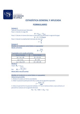
  • 1. ESTADÍSTICA GENERAL Y APLICADA FORMULARIO Semana 1: Tabla de frecuencias por intervalos Paso 1: Calcule el rango (R): 𝑹 = 𝑿𝒎𝒂𝒙 − 𝑿𝒎𝒊𝒏 Paso 2: Calcule el número de clases o intervalos (k) utilizando la regla de Sturges: 𝒌 = 𝟏 + 𝟑. 𝟑 𝒍𝒐𝒈 𝒏 Paso 3: Calcule la amplitud del intervalo de clase (c): 𝒄 = 𝑹 𝒌 Semana 2: Medidas de tendencia central (datos no agrupados) Media aritmética 𝑿 ̅ = ∑ 𝑿𝒊 𝒏 Propiedades de la media aritmética Nueva Variable Nueva Media 𝒚𝒊 = 𝒙𝒊 ± 𝒃 𝒚 ̅ = 𝒙 ̅ ± 𝒃 𝒚𝒊 = 𝒄 𝒙𝒊 𝒚 ̅ = 𝒄𝒙 ̅ 𝒚𝒊 = 𝒄𝒙𝒊 ± 𝒃 𝒚 ̅ = 𝒄𝒙 ̅ ± 𝒃 Mediana Impar: 𝑴𝒆 = 𝒙( 𝒏+𝟏 𝟐 ) Par: 𝑴𝒆 = 𝒙 ( 𝒏 𝟐 ) +𝒙 ( 𝒏 𝟐 +𝟏) 𝟐 Moda (Dato más frecuente) Medidas de tendencia no central (datos no agrupados) Cálculo de percentiles 1. Ordenar los datos en forma ascendente. 2. Hallar la posición (j) del percentil (Pk) a partir de la siguiente expresión: 𝒋 = 𝒌(𝒏 + 𝟏) 𝟏𝟎𝟎 3. Ubicar el percentil en la posición hallada si “j” es un número entero; caso contrario, el percentil se calcula con la siguiente fórmula: 𝑷𝒌 = 𝑳𝒊 + 𝒅𝒆𝒄 × (𝑳𝒅 − 𝑳𝒊)
  • 2. Semana 3: Medidas de variabilidad  Rango: 𝑹 = 𝑿𝒎𝒂𝒙 − 𝑿𝒎𝒊𝒏  Rango Intercuartilico: 𝑹𝑰 = 𝑸𝟑 − 𝑸𝟏  Varianza: 𝒔𝟐 = ∑ 𝑿𝒊 𝟐 −𝒏𝑿 ̅𝟐 𝒏 𝒊=𝟏 𝒏−𝟏  Desviación Estándar: 𝒔 = √𝒔𝟐  Coeficiente de Variación 𝑪𝑽 = 𝑺 𝑿 ̅ × 𝟏𝟎𝟎 Propiedades de la Varianza Nueva Variable Nueva Media Nueva varianza Nueva desviación estándar 𝒚𝒊 = 𝒙𝒊 ± 𝒃 𝒚 ̅ = 𝒙 ̅ ± 𝒃 𝒔𝒚 𝟐 = 𝒔𝒙 𝟐 𝒔𝒚 = 𝒔𝒙 𝒚𝒊 = 𝒄 𝒙𝒊 𝒚 ̅ = 𝒄𝒙 ̅ 𝒔𝒚 𝟐 = 𝒄𝟐 𝒔𝒙 𝟐 𝒔𝒚 = 𝒄𝒔𝒙 𝒚𝒊 = 𝒄𝒙𝒊 ± 𝒃 𝒚 ̅ = 𝒄𝒙 ̅ ± 𝒃 𝒔𝒚 𝟐 = 𝒄𝟐 𝒔𝒙 𝟐 𝒔𝒚 = 𝒄𝒔𝒙 Medidas de Forma  Coeficiente de Asimetría 𝑨𝒌 = 𝟑(𝑿 ̅ − 𝑴𝒆) 𝑺 Medidas de Concentración  Coeficiente de Curtosis. 𝑲𝒖 = 𝑸𝟑 − 𝑸𝟏 𝟐(𝑷𝟗𝟎 − 𝑷𝟏𝟎) = 𝑷𝟕𝟓 − 𝑷𝟐𝟓 𝟐(𝑷𝟗𝟎 − 𝑷𝟏𝟎) Semana 4:  Probabilidad  Experimento aleatorio  Espacio muestral: (Ω)  Eventos: A, B, C…  Operaciones entre eventos. Unión: 𝑨 ∪ 𝑩 Intersección: 𝑨 ∩ 𝑩 Eventos mutuamente excluyentes 𝑨 ∩ 𝑩 = ∅  Probabilidad de un evento: 𝑷(𝑨) = 𝒏 (𝑨) 𝒏(𝜴)  Probabilidad condicional 𝑷(𝑨/𝑩) = 𝑷(𝑨 ∩ 𝑩) 𝑷(𝑩)  Principio de adición para 2 eventos 𝑷(𝑨 ∪ 𝑩) = 𝑷(𝑨) + 𝑷(𝑩) − 𝑷(𝑨 ∩ 𝑩)
  • 3. Semana 5:  Principio de multiplicación para n eventos 𝑷(𝑨𝟏 ∩ 𝑨𝟐 ∩ … ∩ 𝑨𝒏) = 𝑷(𝑨𝟏) 𝑷(𝑨𝟐/𝑨𝟏) … 𝑷(𝑨𝒏/𝑨𝟏 ∩ … ∩ 𝑨𝒏−𝟏)  Eventos independientes para 2 eventos 𝑷(𝑨/𝑩) = 𝑷(𝑨) 𝑷(𝑨 ∩ 𝑩) = 𝑷(𝑨) × 𝑷(𝑩)  Teorema de probabilidad total 𝑷(𝑨) = 𝑷(𝑨𝟏) × 𝑷(𝑨/𝑨𝟏) + 𝑷(𝑨𝟐) × 𝑷(𝑨/𝑨𝟐) + ⋯ + 𝑷(𝑨𝒏) × 𝑷(𝑨/𝑨𝒏)  Teorema de Bayes 𝑷(𝑨𝒊/ 𝑨) = 𝑷(𝑨𝒊 ∩ 𝑨) 𝑷(𝑨) 𝑷(𝑨𝒊/ 𝑨) = 𝑷(𝑨𝒊) × 𝑷(𝑨/𝑨𝒊) 𝑷(𝑨𝟏) × 𝑷(𝑨/𝑨𝟏) + 𝑷(𝑨𝟐) × 𝑷(𝑨/𝑨𝟐) + ⋯ + 𝑷(𝑨𝒏) × 𝑷(𝑨/𝑨𝒏) ;  𝒊 Semana 6: Distribución Binomial  Función de probabilidad de la distribución Binomial. 𝑷(𝑿 = 𝒙) = ∁𝒙 𝒏 𝒑𝒙(𝟏 − 𝒑)𝒏−𝒙 Medidas de resumen. Esperanza Matemática 𝑬(𝑿) = 𝒏 𝒑 Varianza 𝑽(𝑿) = 𝒏 𝒑(𝟏 − 𝒑) Distribución Poisson  Función de probabilidad de la distribución Poisson. 𝑷(𝑿 = 𝒙) = 𝒆−𝝀 × 𝝀𝒙 𝒙! Medidas de resumen. Esperanza Matemática 𝑬(𝑿) = 𝝀 Varianza 𝑽(𝑿) = 𝝀 Semana 7: Distribución normal  Estandarización 𝒁 = 𝑿 − 𝝁 𝝈 ESTADISTICA APLICADA Semana 1: Estimación por intervalo para la media o promedio poblacional 𝝁:  Caso I: Cuando σ2 es conocido: 𝑰𝑪(𝝁) = 〈𝒙 ̅ ± 𝒁𝟏−𝜶 𝟐 ⁄ 𝝈 √𝒏 〉  Caso II: Cuando σ2 es desconocido (n≤ 30) 𝑰𝑪(𝝁) = 〈𝒙 ̅ ± 𝒕𝟏−𝜶 𝟐 ⁄ ;𝒏−𝟏 𝑺 √𝒏 〉  Caso III: Cuando σ2 es desconocido (n> 30) 𝑰𝑪(𝝁) = 〈𝒙 ̅ ± 𝒛𝟏−𝜶 𝟐 ⁄ 𝑺 √𝒏 〉
  • 4. Estimación por intervalo para la proporción poblacional 𝝅: 𝑰𝑪(𝝅) = 𝒑 ± 𝒁𝟏−𝜶 𝟐 ⁄ √ 𝒑(𝟏 − 𝒑) 𝒏 Estimación por intervalo para la varianza poblacional 𝝈𝟐 : (𝒏 − 𝟏)𝒔𝟐 𝝌𝟏−𝜶 𝟐 ⁄ ;𝒏−𝟏 𝟐 ≤ 𝝈𝟐 ≤ (𝒏 − 𝟏)𝒔𝟐 𝝌𝜶 𝟐 ⁄ ;𝒏−𝟏 𝟐 Tamaño de muestra Media 𝒏𝟎 = 𝒛𝟏−𝜶 𝟐 ⁄ 𝟐 × 𝝈𝟐 𝜺𝟐 Proporción: 𝒏𝟎 = 𝒛𝟏−𝜶 𝟐 ⁄ 𝟐 𝒑(𝟏 − 𝒑) 𝜺𝟐 Factor de corrección si se conoce la población 𝒏 = 𝒏𝟎 𝟏 + 𝒏𝟎 𝑵 Semana 2: Intervalo de confianza para el cociente de varianzas (𝝈𝟏 𝟐 𝝈𝟐 𝟐 ⁄ ) 〈 𝒔𝟏 𝟐 𝒔𝟐 𝟐 × 𝟏 𝑭𝜶 𝟐 ⁄ , 𝒏𝟏−𝟏; 𝒏𝟐−𝟏 ≤ 𝝈𝟏 𝟐 𝝈𝟐 𝟐 ≤ 𝒔𝟏 𝟐 𝒔𝟐 𝟐 × 𝑭𝜶 𝟐 ⁄ , 𝒏𝟐−𝟏; 𝒏𝟏−𝟏〉 Intervalo de confianza para las diferencias de medias poblacionales (𝝁𝟏 − 𝝁𝟐)  Caso 1: Cuando las varianzas poblacionales son conocidas 𝑰𝑪(𝝁𝟏 − 𝝁𝟐) : (𝒙 ̅ − 𝒚 ̅) ± 𝒛𝟏−𝜶 𝟐 ⁄ √ 𝝈𝟏 𝟐 𝒏𝟏 + 𝝈𝟐 𝟐 𝒏𝟐  Caso 2: Cuando las varianzas poblacionales son desconocidas pero homogéneas 𝑰𝑪(𝝁𝟏 − 𝝁𝟐) : (𝒙 ̅ − 𝒚 ̅) ± 𝒕𝟏−𝜶 𝟐 ⁄ ;𝒏𝟏+𝒏𝟐−𝟐 √( (𝒏𝟏 − 𝟏)𝒔𝟏 𝟐 + (𝒏𝟐 − 𝟏)𝒔𝟐 𝟐 𝒏𝟏 + 𝒏𝟐 − 𝟐 ) ( 𝟏 𝒏𝟏 + 𝟏 𝒏𝟐 )  Caso 3: Cuando las varianzas poblacionales son desconocidas, pero no homogéneas 𝑰𝑪(𝝁𝟏 − 𝝁𝟐) : (𝒙 ̅ − 𝒚 ̅) ± (𝒕𝟏−𝜶 𝟐 ⁄ ; 𝒈 ) √ 𝒔𝟏 𝟐 𝒏𝟏 + 𝒔𝟐 𝟐 𝒏𝟐 Grados de libertad 𝒈 = [ 𝒔𝟏 𝟐 𝒏𝟏 + 𝒔𝟐 𝟐 𝒏𝟐 ] 𝟐 [ 𝒔𝟏 𝟐 𝒏𝟏 ] 𝟐 𝒏𝟏 + 𝟏 + [ 𝒔𝟐 𝟐 𝒏𝟐 ] 𝟐 𝒏𝟐 + 𝟏 − 𝟐 Intervalo de confianza para la diferencia de 2 proporciones poblacionales (𝝅𝟏 − 𝝅𝟐)
  • 5. 𝑰𝑪(𝝅𝟏 − 𝝅𝟐) : (𝒑 𝟏 − 𝒑𝟐) ± 𝒛𝟏−𝜶 𝟐 ⁄ √ 𝒑𝟏(𝟏 − 𝒑𝟏) 𝒏𝟏 + 𝒑𝟐(𝟏 − 𝒑𝟐) 𝒏𝟐 Semana 3: PROCEDIMIENTO PARA REALIZAR UNA PRUEBA DE HIPÓTESIS Paso 1 (Plantee las hipótesis de prueba) Paso 2 (Establezca el nivel de significancia) α Paso 3 (Calcule el valor del estadístico de prueba) La decisión de aceptar o rechazar la hipótesis nula, se hace en base al valor del estadístico de contraste (estadístico de prueba), este valor se obtiene con los datos de la muestra. Paso 4 Regla de decisión La región de rechazo, también conocida como región crítica, se establece a partir del nivel de significancia α. Paso 5 (Concluya de acuerdo al enunciado del problema) Si el valor del estadístico de prueba cae en la región de rechazo, se rechaza la hipótesis nula (H0), caso contrario no se rechaza. Prueba de Hipótesis para la media poblacional:  CASO 1: Cuando σ es conocido 𝒁𝒄𝒂𝒍 = 𝒙 ̅ − 𝝁𝟎 𝝈 √𝒏 ~𝑵(𝟎, 𝟏)  CASO 2: Cuando σ es desconocido y n ≤ 30 𝑻𝒄𝒂𝒍 = 𝒙 ̅ − 𝝁𝟎 𝒔 √𝒏 ~𝒕𝒏−𝟏  CASO 3: Cuando σ es desconocido y n > 30 𝒁𝒄𝒂𝒍 = 𝒙 ̅ − 𝝁𝟎 𝒔 √𝒏 ~𝑵(𝟎, 𝟏) Prueba de Hipótesis para la proporción poblacional: 𝒁𝒄𝒂𝒍 = 𝒑 − 𝝅𝟎 √𝝅𝟎(𝟏 − 𝝅𝟎) 𝒏 ~𝑵(𝟎, 𝟏) 𝒑 = ∑ 𝑿𝒊 𝒏 𝒊=𝟏 𝒏 = 𝑿𝟏 + 𝑿𝟐 + ⋯ 𝑿𝒏 𝒏 Prueba de Hipótesis para la varianza poblacional: 𝝌𝒄𝒂𝒍 𝟐 = (𝒏 − 𝟏)𝒔𝟐 𝝈𝟎 𝟐 ~𝝌𝒏−𝟏 𝟐
  • 6. Semana 4: Prueba de hipótesis para el cociente de varianzas poblacionales: 𝑭𝒄𝒂𝒍 = 𝒔𝟏 𝟐 𝒔𝟐 𝟐 ~𝑭𝒏𝟏−𝟏, 𝒏𝟐−𝟏 Prueba de hipótesis para la diferencia de medias poblacionales:  Caso 1: Cuando las varianzas poblacionales son conocidas 𝒁𝒄𝒂𝒍 = (x ̅1 − x ̅2) − μ0 √ 𝜎1 2 𝑛1 + 𝜎2 2 𝑛2  Caso 2: Cuando las varianzas poblacionales son desconocidas pero homogéneas 𝒕𝒄𝒂𝒍 = (𝒙 ̅𝟏 − 𝒙 ̅𝟐) − 𝝁𝟎 √ (𝒏𝟏 − 𝟏)𝑺𝟏 𝟐 + (𝒏𝟐 − 𝟏)𝑺𝟐 𝟐 𝒏𝟏 + 𝒏𝟐 − 𝟐 ( 𝟏 𝒏𝟏 + 𝟏 𝒏𝟐 )  Caso 3: Cuando las varianzas poblacionales son desconocidas, pero no homogéneas 𝒕𝒄𝒂𝒍 = (x ̅1 − x ̅2) − μ0 √ 𝑆1 2 𝑛1 + 𝑆2 2 𝑛2 Grados de libertad 𝒈 = ( 𝒔𝟏 𝟐 𝒏𝟏 + 𝒔𝟐 𝟐 𝒏𝟐 ) 𝟐 ( 𝒔𝟏 𝟐 𝒏𝟏 ) 𝟐 𝒏𝟏 + 𝟏 + ( 𝒔𝟐 𝟐 𝒏𝟐 ) 𝟐 𝒏𝟐 + 𝟏 − 𝟐 Prueba de hipótesis para la diferencia de proporciones (𝝅𝟏 − 𝝅𝟐) = 𝝅𝟎 Prueba de hipótesis para la igualdad de proporciones Zcal = 𝑝1 − 𝑝2 √𝑝̂(1 − 𝑝̂) ( 1 𝑛1 + 1 𝑛2 ) 𝑝̂ = 𝑛1𝑝1 + 𝑛2𝑝2 𝑛1 + 𝑛2 Prueba de hipótesis para la diferencia de proporciones diferentes de cero 𝒁𝒄𝒂𝒍 = (𝒑𝟏 − 𝒑𝟐) − 𝝅𝒐 √ 𝒑𝟏(𝟏 − 𝒑𝟏) 𝒏𝟏 + 𝒑𝟐(𝟏 − 𝒑𝟐) 𝒏𝟐
  • 7. Semana 5: Análisis de varianza (ANOVA) 𝐻0:𝜇1 = 𝜇2 = 𝜇3 = ⋯ = 𝜇𝑘 𝐻1:𝐴𝑙 𝑚𝑒𝑛𝑜𝑠 𝑢𝑛 𝜇𝑖 es diferente Fcal = CMTra CME ~ 𝐹𝑘−1; 𝑛−𝑘; 𝛼 Cuadro ANOVA Fuente de variación Grados de libertad Suma de cuadrados Cuadrados medios Fcal Tratamiento k – 1 SCTra = ∑ T.j 2 𝑛𝑗 − T.. 2 𝑛 k j=1 CMTra = SCTra 𝑘 − 1 Fcal = CMTra CME Error n – k SCE = SCT − SCTra CME = SCE 𝑛 − 𝑘 Total n – 1 SCT = ∑ ∑ 𝑦ij 2 𝑟 i=1 𝑘 j=1 − T.. 2 𝑛 Semana 6: Prueba de Independencia 𝜒𝑐𝑎𝑙 2 = ∑ ∑ (𝑜𝑖𝑗 − 𝑒𝑖𝑗)2 𝑒𝑖𝑗 𝑐 𝑗=1 𝑟 𝑖=1 ~ 𝜒[1−𝛼; (𝑟−1)×(𝑐−1)] 2 r=Número de categorías de la variable X c=Número de categorías de la variable Y Frecuencia esperada 𝒆𝒊𝒋 = 𝒏𝒊. × 𝒏.𝒋 𝒏.. Coeficiente de contingencia 𝐶 = √ 𝜒𝑐𝑎𝑙 2 𝜒𝑐𝑎𝑙 2 + 𝑛 Prueba de homogeneidad 𝜒𝑐𝑎𝑙 2 = ∑ ∑ (𝑜𝑖𝑗 − 𝑒𝑖𝑗)2 𝑒𝑖𝑗 𝑘 𝑗=1 𝑟 𝑖=1 ~ 𝜒[1−𝛼, (𝑟−1)×(𝑘−1)] 2 r=Número de categorías de la variable k=Número de poblaciones
  • 8. Semana 7: Regresión lineal simple 𝑺𝑪(𝒙) = ∑ 𝒙𝟐 − 𝒏𝒙 ̅𝟐 𝑺𝑪(𝒚) = ∑ 𝒚𝟐 − 𝒏𝒚 ̅𝟐 𝑺𝑷(𝒙𝒚) = ∑ 𝒙𝒚 − 𝒏 𝒙 ̅ 𝒚 ̅  Estimación de los parámetros del modelo de regresión lineal simple 𝒀 ̂ = 𝒃𝟎 + 𝒃𝟏𝑿 𝜷 ̂𝟏 = 𝒃𝟏 = 𝑺𝑷(𝒙, 𝒚) 𝑺𝑪(𝒙) 𝜷 ̂𝟎 = 𝒃𝟎 = 𝒚 ̅ − 𝒃𝟏𝒙 ̅ Prueba de hipótesis para validar el modelo Paso 1 (Plantee las hipótesis de prueba) 𝑯𝟎: 𝜷𝟏 = 𝟎 (La recta de regresión no es significativa) 𝑯𝟏: 𝜷𝟏 ≠ 𝟎 (La recta de regresión es significativa) Paso 2 (Establezca el nivel de significancia) α Paso 3 (Calcule el valor del estadístico de prueba) 𝑻𝒄𝒂𝒍 = 𝒃𝟏 𝑺𝒃𝟏 ~𝒕𝒏−𝟐 𝑺𝒃𝟏 = 𝑺𝒆 √𝑺𝑪(𝑿) 𝑺𝒆 = √ ∑ 𝒚𝒊 𝟐 𝒏 𝒊=𝟏 − 𝒃𝟎 ∑ 𝒚𝒊 𝒏 𝒊=𝟏 − 𝒃𝟏 ∑ 𝒙𝒊𝒚𝒊 𝒏 𝒊=𝟏 𝒏 − 𝟐 Coeficiente de correlación: 𝑟 = 𝑆𝑃(𝑥, 𝑦) √𝑆𝐶(𝑥) √𝑆𝐶(𝑦) ; −1 ≤ 𝑟 ≤ 1 Coeficiente de determinación 𝑅2 = 𝑏1𝑆𝑃(𝑥, 𝑦) 𝑆𝐶(𝑦) ; 0 ≤ 𝑅2 ≤ 1