Round Robin and Priority scheduling algorithm implementation - C code

1. Priority Scheduling
Priority scheduling is one of the most common scheduling algorithms in batch systems. Each
process is assigned a priority. Process with the highest priority is to be executed first and so on.
Processes with the same priority are executed on first come first served basis. Priority can be
decided based on memory requirements, time requirements or any other resource requirement.
Implementation:
1. First input the processes with their burst time and priority.
2. Sort the processes, burst time and priority according to the
priority.
3. Now simply apply FCFS algorithm.
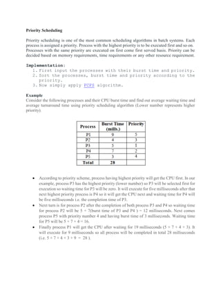
Example
Consider the following processes and their CPU burst time and find out average waiting time and
average turnaround time using priority scheduling algorithm (Lower number represents higher
priority).
 According to priority scheme, process having highest priority will get the CPU first. In our
example, process P3 has the highest priority (lower number) so P3 will be selected first for
execution so waiting time for P3 will be zero. It will execute for five milliseconds after that
next highest priority process is P4 so it will get the CPU next and waiting time for P4 will
be five milliseconds i.e. the completion time of P3.
 Next turn is for process P2 after the completion of both process P3 and P4 so waiting time
for process P2 will be 5 + 7(burst time of P3 and P4 ) = 12 milliseconds. Next comes
process P5 with priority number 4 and having burst time of 3 milliseconds. Waiting time
for P5 will be 5 + 7 + 4 = 16.
 Finally process P1 will get the CPU after waiting for 19 milliseconds (5 + 7 + 4 + 3). It
will execute for 9 milliseconds so all process will be completed in total 28 milliseconds
(i.e. 5 + 7 + 4 + 3 + 9 = 28 ).

2. It can be represented in gantt chart as follow:
Process Burst Time Priority
Waiting
Time
Completion
Time
Turnaround
Time
P1 9 5 19 – 0 = 19 28 9 + 19 = 28
P2 4 3 12 - 0 = 12 16 4 + 12 = 16
P3 5 1 0 - 0 = 0 5 5 + 0 = 5
P4 7 2 5 - 0 = 5 12 7 + 5 = 12
P5 3 4 16 - 0 = 16 19 3 + 16 = 19
Total 52 80 80
Average 10.4 16 16
Round-Robin Scheduling
Round Robin(RR) scheduling algorithm is mainly designed for time-sharing systems. This
algorithm is similar to FCFS scheduling, but in Round Robin(RR) scheduling, preemption is added
which enables the system to switch between processes.
1. A fixed time is allotted to each process, called a quantum, for execution.
2. Once a process is executed for the given time period that process is preempted and another
process executes for the given time period.
3. Context switching is used to save states of preempted processes.
4. This algorithm is simple and easy to implement and the most important is thing is this
algorithm is starvation-free as all processes get a fair share of CPU.
5. It is important to note here that the length of time quantum is generally from 10 to 100
milliseconds in length.
Steps to find waiting times of all processes:
1. Create an array rem_bt[] to keep track of remaining burst
time of processes. This array is initially a copy of bt[]
(burst times array)
2. Create another array wt[] to store waiting times of
processes. Initialize this array as 0.
3. Initialize time : t = 0
4. Keep traversing the all processes while all processes are
not done. Do following for i'th process if it is not done
yet.
a. If rem_bt[i] > quantum
(i) t = t + quantum
bt_rem[i] -= quantum;

3. b. Else // Last cycle for this process
t = t + bt_rem[i];
wt[i] = t - bt[i]
bt_rem[i] = 0; // This process is over
Once we have waiting times, we can compute turn around time tat[i]
of a process as sum of waiting and burst times, i.e., wt[i] +
bt[i]
Example
Process Burst Time
P1 5
P2 4
P3 1
P4 6
Time Slice=2ms
P1 P2 P3 P4 P1 P2 P4 P1 P4
0 2 4 5 7 9 11 13 14 16
Process Burst Time Waiting Time
Completion
Time
Turnaround
Time
P1 5
(0 - 0) + (7 - 2) +
(13 - 9) = 9
14 14
P2 4
(2 - 0) + (9 - 4) =
7
11 11
P3 1 (4 - 0) = 4 5 5
P4 6
(5 - 0) + (11 - 7)
+ (14 - 13) = 10
16 16
Total 30 46 46
Average 7.5 11.5 11.5