Perceptrone Adaline Madaline Hetero Associative Auto Associative Discrete Hopfield Back propagation

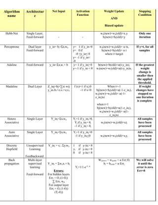
1. Algorithm Architectur Net Input Activation Weight Update Stopping
name e Function Condition
AND
Biased update
Hebb-Net Single Layer, wij(new)=wij(old)+xi y Only one
Feed-forward - - bj(new)=bj(old)+y iteration
Perceptrone Dual layer y_in= bj+Σxiwij y= 1 if y_in>θ wij(new)=wij(old)+ α txi If y=t, for all
Feed-forward y= 0 if bj(new)=bj(old)+ α t samples
-θ ≤y_in≤ θ where t=target
y= -1 if y_in<
-θ
Adaline Feed-forward y_in=Σxiwi + b y= 1 if y_in≥ θ b(new)=b(old)+α(t-y_in), If the greatest
y=-1 if y_in < θ wi(new)=wi(old)+α(t-y_in)xi weight
change is
smaller then
the applied
threshold.
Madaline Dual Layer Z_inj=bj+∑xi wij f (x)=1 if x>0 When t=-1 If weight
y_in=b3+z1v1+z2v2 -1 if x<0 bj(new)=bj(old)+α(-1-z_inj), changes have
wij(new)=wij(old)+ α(-1- stopped so
z_inj)xi one Iteration
is complete
when t=1
bj(new)=bj(old)+α(1-z_inj),
wij(new)=wij(old)+ α(1-
z_inj)xi
Hetero Single Layer Y_inj=Σxiwij Yj=1 if y_inj>θj All samples
Associative Yj if y_inj= θj wij(new)=wij(old)+sitj have been
-1 if y_inj< θj processed
Auto Single Layer Y_inj=Σxiwij Yj=1 if y_inj>0 All samples
Associative -1 if y_inj<0 wij(new)=wij(old)+xiyj have been
processed
Discrete Unsupervised Y_inj = xi + Σyiwji 1 if y-ini> θ
Hopfield Learning yi if y-ini= θ
0 if y-ini< θ
Feedbackward
Back Multi-layer Wij(new) = wij(old) + α Errj Oi We will solve
propagation supervised Y_inj = Σwijxi + bj bj = bj(old) + α Errj it until the
learning Yj=1/1-e-Y_in error is zero
Errors: Err=0
Feed-forward For hidden layers
Errj = Oj (1-Oj)
∑ Errk wjk
For output layer
Errj = Oj (1-Oj)
(Tj-Oj)

2. Self unsupervised Dj=∑(wij-xi)2 Choose the Wij(new)= Wij(old)+α[xi-wij(old)]
Organization learning minimum Dj (new)= 0.5 α (old)
map and set the If
Feed- value of j convergence
Forward according to criterion met,
it. STOP.
Or
When cluster
1 and cluster
2 is inverse of
each other.