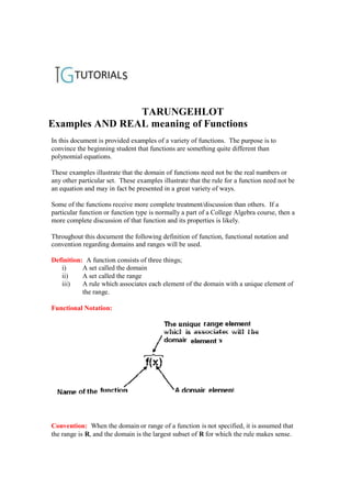
1. TARUNGEHLOT
Examples AND REAL meaning of Functions
In this document is provided examples of a variety of functions. The purpose is to
convince the beginning student that functions are something quite different than
polynomial equations.
These examples illustrate that the domain of functions need not be the real numbers or
any other particular set. These examples illustrate that the rule for a function need not be
an equation and may in fact be presented in a great variety of ways.
Some of the functions receive more complete treatment/discussion than others. If a
particular function or function type is normally a part of a College Algebra course, then a
more complete discussion of that function and its properties is likely.
Throughout this document the following definition of function, functional notation and
convention regarding domains and ranges will be used.
Definition: A function consists of three things;
i) A set called the domain
ii) A set called the range
iii) A rule which associates each element of the domain with a unique element of
the range.
Functional Notation:
Convention: When the domain or range of a function is not specified, it is assumed that
the range is R, and the domain is the largest subset of R for which the rule makes sense.

2. 1

3. I) Some Very Simple Functions
The domains and rule of the three functions shown in
these diagrams are quite simple, but they are indeed
functions.
Moreover view of functions consisting of two sets
with arrows from elements of the domain to elements
of the range will serve well to help understand
functions in general
The example below shows quite clearly that the
domain and range of a function need not be sets of
numbers. In most College Algebra courses the
functions discussed do have domains and ranges
which are sets of numbers, but that is not a
requirement of the definition of function.
II) Linear Functions
Definition: A linear function is a function whose domain is R, whose range is R, and
whose rule can be expressed as a linear equation.
Recall a linear equation in two variables is an equation which can be written as
y = mx + b where m and b are real numbers.
This leads to the following alternate preferred definition for a linear function.
Definition: A linear function is a function whose domain is R, whose range is R, and
whose rule can be written as f(x) = mx + b where x is a domain element, m R and
b R.
Comment: Linear functions are a special case of the more general class of functions
called polynomial functions. Thus the set of linear functions is a subset of the set of
polynomial functions.
2

4. Example: Let f be the function whose rule is f(x) = 3x + 5.
Convention dictates that the range of this function is R and because the rule makes sense
for every real number substituted into the rule, the domain is also R. The rule is written
as a linear equation, so it follows that f is a linear function.
Graph of Linear Equation Graph of Linear Function
Comment: The word linear is now being used as an important adjective in four distinct
contexts. We speak of linear polynomials, linear equations in one variable, linear
equations in two variables, and linear functions.
A linear polynomial is an expression which can be written as ax + b where a and b
are real numbers. A linear polynomial is a mathematical creature just like natural
numbers, rational numbers, irrational numbers, matrices, and vectors are
mathematical creatures. There is no equation involved. The concept of solving a
linear polynomial is meaningless. The arithmetic-like concepts of addition,
multiplication, and subtraction in the context of all polynomials as well as linear
polynomials does have meaning.
A linear equation in one variable is an equation which can be written as ax + b = 0
where a and b are real numbers. The graph of a linear equation in one variable is
a sngle point on the x-axis unless a = 0 and b ≠ 0 in whi ch case there are no
solutions and hence no graph.
A linear equation in two variables is an equation which can be written in the form
y = mx + b where m and b are real numbers. This is called the slope-intercept
form of the equation of a line. The graph of a linear equation in two variables is a
line. The coefficient m is the slope of the graph and b is the y-intercept of that
graph.
A linear function is a function whose domain is R, whose range is R, and whose
rule may be written as f(x) = mx + b where a and b are real numbers. The graph
of a linear function is a non-vertical line with slope m and y-intercept b. A linear
3

5. function is a mathematical creature just like natural numbers, rational numbers ,
irrational numbers, matrices, vectors, and linear polynomials are mathematical
creatures. The concept of solving a linear function is meaningless. The
arithmetic-like concepts of addition, multiplication, and subtraction in the context
of all functions as well as linear functions does have meaning. A variety of
additional facts peculiar to functions will be studied in this course.
III) Quadratic Functions
Definition: A quadratic function is a function whose domain is R, whose range is R, and
whose rule can be expressed as a quadratic equation.
Recall that a quadratic equation in two variables is an equation that can be written
y = ax2 + bx + c where a, b, and c are real numbers and a ≠ 0.
This leads to the following alternate preferred definition for a quadratic function.
Definition: A quadratic function is a function whose domain is R, whose range is R, and
2
whose rule can be written as f(x) = ax + bx + c where a, b, and c are real numbers and
a ≠ 0.
Comment: Quadratic functions are a special case of the more general class of functions
called polynomial functions. Thus the set of quadratic functions is a subset of the set of
polynomial functions.
2
Example: Let f be the function whose rule is f(x) = x + x - 6.
The convention dictates that the range of this function is R and because the rule makes
sense for every real number substituted into the rule, the domain is also R. The rule is
written as a quadratic equation, so it follows that f is a quadratic function.
Graph of Quadratic Equation Graph of Quadratic Function
4

6. Comment: The word quadratic is now being used as an important adjective in four
distinct contexts. We speak of quadratic polynomials, quadratic equations in one
variable, quadratic equations in two variables, and quadratic functions.
A quadratic polynomial is an expression which can be written as ax 2 + bx + c
where a and b are real numbers. A quadratic polynomial is a mathematical
creature just like natural numbers, rational numbers, irrational numbers, matrices,
vectors, linear polynomials, and linear functions are mathematical creatures. There
is no equation involved. The concept of solving a quadratic polynomial is
meaningless. The arithmetic-like concepts of addition, multiplication, and
subtraction in the context of all polynomials as well as quadratic polynomials do
have meaning.
A quadratic equation in one variable is an equation which can be written as ax2 +
bx + c = 0 where a, b, and c are real numbers. The graph of a quadratic equation
in one variable may be a sngle point, or two points on the x -axis. If the
discriminant of the quadratic polynomial is negative the quadratic equation in one
variable has no real solutions and hence has no graph.
A quadratic equation in two variables is an equation which can be written in the
form y = ax2 + bx + c where a, b, and c are real numbers and a ≠ 0. The graph of
a quadratic equation in two variables is a parabola which opens up if the leading
coefficient is positive and opens down if the leading coefficient is negative.
A quadratic function is a function whose domain is R, whose range is R, and
2
whose rule may be written as f(x) = ax + bx + c where a, b, and c are real
numbers and a ≠ 0. The graph of a quadratic function is a parabola which opens
up if a > 0 and opens down if a < 0. A quadratic function is a mathematical
creature just like natural numbers, rational numbers, irrational numbers, matrices,
vectors, and linear polynomials are mathematical creatures. The concept of solving
a linear function is meaningless. The arithmetic-like concepts of addition,
multiplication, and subtraction in the context of all functions as well as quadratic
functions do have meaning. A variety of additional facts peculiar to functions
will be studied in this course.
IV) Polynomial Functions
Definition: A polynomial function is a function whose domain is R, whose range is R,
and whose rule can be expressed as a polynomial equation.
Recall that a polynomial equation in two variables is an equation that can be written
y an x n an 1x n 1 a1x a 0 where n is a whole number and each of the coefficients
ai is a real number.
This leads to the following alternate preferred definition for a quadratic function.
5

7. Definition: A polynomial function is a function whose domain is R, whose range is R,
and whose rule can be expressed as f ( x) a nx n an 1 x n 1 a1 x a0 where n is a
whole number and each of the coefficients a i is a real number.
Examples: Every linear function is a polynomial function.
Examples: Every quadratic function is a polynomial function.
5 2
Example: Let f be the function whose rule is f(x) = x + 3x – 6x + 9.
Convention dictates that the range of this function is R and because the rule makes sense
for every real number substituted into the rule, the domain is also R. The rule is written
as a polynomial equation, so it follows that f is a polynomial function.
Polynomial functions will be a major topic of study in College Algebra.
V) Absolute Value Function
Definition: The absolute value function abs is the function whose rule is given by
x if x 0
abs (x )
x if x 0
Convention dictates that the range of this function is R and
because the rule makes sense for every real number
substituted into the rule, the domain is also R.
The graph of abs is shown at the right.
The name abs is less used in discussions involving the
absolute value function. The more familiar notation
| x | is usually used in lieu of abs(x).
VI) Sequences
Definition: A sequence is a function whose domain is the set of Natural Numbers N.
The definition of sequence is pretty simply stated, but there are many special
consequences of the fact that the domain of a sequence is N. Sequences have been
studied for centuries. Sequences have been studied with and without the concept of
function. Quite a bit of special (mostly historical in origin) terminology and notation is
used in a discussion of sequences.
When working with sequences, range elements are frequently called terms of the
sequence. For example:
The range element associated with the domain element 1 is called the first term of
the sequence.
6

8. The range element associated with the domain element 6 is called the sixth term
of the sequence.
The range element associated with the domain element n is called the n th term of
the sequence.
Because the domain of every sequence is N, the graph of a sequence will consist of a set
of discrete points.
Because the domain of every sequence is N, it is possible to speak of the first domain
element.
Because the domain of every sequence is N, it is possible to speak of the next domain
element.
Because the domain of every sequence is N, it is not possible to speak of the last domain
element.
Because the domain of every sequence is N, it is possible to ask about and compute the
sum of the first k terms. This is usually called the kth partial sum of the sequence.
Definition: The nth partial sum of a sequence is defined to be the sum of the first n terms
of the sequence.
VI - A) Tau
The function whose name is the Greek letter τ (pronounced tau) is a function whose
domain is the Natural Numbers N. So τ is a sequence. The rule for τ is not given by a
formula. The rule for τ is: τ(n) is the number of positive divisors of n.
To compute the range value associated with a particular domain element n, it is necessary
to determine all positive divisors of n and simply count them. It is convenient to think of
τ simply as a function which counts the number of positive divisors of domain elements.
τ(1) = 1 τ(2) = 2 τ(3) = 2 τ (4) = 3 τ (5) = 2 τ (6) = 4
τ(7) = 2 τ(8) = 4 τ(9) = 3 τ (10) = 4 τ (11) = 2 τ (12) = 6
The graph of the first 12 terms of Tau consists of the points:
(1, 1) (2, 2) (3, 2) (4, 3) (5, 2) (6, 4)
(7, 2) (8, 4) (9, 3) (10, 4) (11, 2) (12, 6)
Notice that if p is a prime number, then τ(p) = 2 and if k is a composite number, then
τ(k) > 2. τ is used to define prime numbers as:
In fact sometimes
Definition: A natural number p is prime if and only if τ (p) = 2.
Notice how neatly this definition prohibits classifying 1 as a prime number.
7

9. VI - B) Sigma
The function whose name is the Greek letter σ (pronounced sigma) is a function whose
domain is the Natural Numbers N. So σ is a sequence. The rule for σ is not given by a
formula. The rule for σ is: σ(n) is the sum of the positive divisors of n.
To compute the range value associated with a particular domain element n, it is necessary
to determine all positive divisors of n and simply add them.
σ (1) = 1 σ (2) = 3 σ (3) = 4 σ (4) = 7 σ (5) = 6 σ (6) = 12
σ (7) = 8 σ (8) = 15 σ (9) = 13 σ (10) = 18 σ (11) = 12 σ (12) = 28
The graph of the first 12 terms of Sigma consists of the points:
(1, 1) (2, 3) (3, 4) (4, 7) (5, 6) (6, 12)
(7, 8) (8, 15) (9, 13) (10, 18) (11, 12) (12, 28)
VI - C) Fibonacci Sequence
Definition: The Fibonacci sequence F is the function whose domain is N and whose rule
is given recursively by: F(1) = 1, F(2)= 1, and for n > 2, F(n) = F(n – 1) + F(n – 2)
F(1) = 1 F(2) = 1 F(3) = 2 F(4) = 3 F(5) = 5 F(6) = 8
F(7) = 13 F(8) = 21 F(9) = 34 F(10) = 55 F(11) = 89 F(12) = 1 44
The graph of the first 12 terms of the Fibonacci sequence consists of the points:
(1, 1) (2, 1) (3, 2) (4, 3) (5, 5) (6, 8)
(7, 13) (8, 21) (9, 34) (10, 55) (11, 89) (12, 144)
VI - D) Arithmetic Sequences
Definition: An arithmetic sequence is a sequence whose consecutive terms have a
common difference.
Equivalent Definition: An arithmetic sequence f is a function whose rule may be
expressed as a linear equation of the form f(n) = dn + b where d is the common difference
and b is the difference f(1) – d.
Comments: Compare the equivalent definition of an arithmetic sequence with the
definition of a linear function.
The domain of a linear function is R The domain of an arithmetic sequence is N
The rule for a linea r function is f(x) = mx + b
The rule for an arithmetic sequence is f(x) = dx + b
The number b in the rule for an arithmetic sequence is the range value associated with 0
( if there were such a range element) so it corresponds exactly to the y-intercept of the
linear function.
8

10. The common difference d is nothing more than the slope as you move from one range
element to the next. The slope of the line joining two terms (x, f(x)) and (x + 1, f(x + 1))
f ( x 1) f ( x) d
of the sequence is given by d.
( x 1) x 1
A casual approach is to view an arithmetic sequence as a linear function with domain N.
Comment: Given any two pieces of information about an arithmetic sequence it is
possible to determine its rule. The next three problem types illustrate the point.
Problem Type 1: If you are given the common difference and the first term of the
arithmetic sequence, then it is possible to write the rule for the function. This is
comparable to the slope-intercept situation/problem when working with linear functions.
Example: Suppose an arithmetic sequence named h has a common difference 8 and the
first term is -5. Find the rule for the function h.
Solution: Snce the function is an arithmetic sequence its rule is of the form
h(n) = dn + b. In our case the common difference d is 8, the rule for h has the form
h(n) =8n + b. Because the first term is -5, b = -5 – 8 = -13 and the rule for the desired
arithmetic sequence is given by h(n) = 8n – 13.
Problem Type 2: If you are given the common difference d and one term of an
arithmetic sequence, then it is possible to write the rule for the function. This is
comparable to the point-slope situation/problems when working with linear functions.
Example: Suppose an arithmetic sequence named h has a common difference 3 and the
fifth term is 12. Find the rule for the function h.
Solution: Snce the function is an arithmetic sequence its rule is of the form
h(n) = dn + b. In our case the common difference d is 3, the rule for h has the form
h(n) =3n + b. Because the fifth term is 12, h(5) = 12, but according to the partially
determined rule h(5) = 3(5) + b = 15 + b. These two representations for h(5) yield the
equation 12 = 15 + b. Clearly then b = -3 and the rule for the desired arithmetic sequence
is given by h(n) = 3n – 3.
Problem Type 3: If you are given two terms of an arithmetic sequence, then it is
possible to write the rule for the function. This is comparable to the two point
situation/problems when working with linear functions.
Example: Suppose the fourth term an arithmetic sequence named k is 10 and the seventh
term is 28. Find the rule for the function h.
Solution: Snce the function is an arithmetic sequence its rule is of the form
h(n) = dn + b. The difference between the seventh and fourth terms is 3d and is also
equal to 28 – 10 = 18. That means 3d = 18 and so the common difference d is 6.
The rule for h has the form h(n) =6n + b. Because the fourth term is 10, h(4) = 10, but
according to the partially determined rule h(4) = 6(4) + b = 24 + b. These two
representations for h(4) yield the equation 10 = 24 + b. Clearly then b = -14 and the rule
for the desired arithmetic sequence is given by h(n) = 6n – 14.
th
Comment: The formula for the n partial sum of an arithmetic sequence named a is:
n
Sn a an
1
2
9

11. VI - D) Mod Functions
The function named mod6
The name of this function is mod6. The domain of mod6 is the set of all natural numbers.
The range of mod 6 is the set 0,1, 2, 3, 4, 5 . Because the domain of mod6 is N, mod 6 is a
sequence. The rule for mod6 is given by:
mod 6(n) is the remainder when n is divided by 6.
To see that mod6 is a function, we refer back to the “arrow” concept of function. The fact
that every natural number may be divided by 6 insures that an arrow emanates from each
element of the domain.
The division algorithm states that for any natural number n there is a unique quotient q
and a unique remainder r such that r 0,1, 2, 3, 4, 5 .
The fact that r 0,1, 2, 3, 4, 5 insures that the arrows end in the range and the fact that
the remainder is unique insures that only one arrow emanates for each domain element.
Therefore mod 6 is a function.
Here are examples of range elements associated with some domain elements
mod 6(3) = 3 mod 6(8) = 2 mod 6(17) = 5 mod 6(424) = 4
The function named mod11
The name of this function is mod11. The domain of mod11 is the set of all natural numbers.
The range of mod11 is the set 0,1, 2, 3, 4, 5, 6, 7, 8, 9,10 . Because the domain of
mod 11 is N, mod11 is a sequence. The rule for mod 11 is given by:
mod 11(n) is the remainder when n is divided by 11.
To see that mod11 is a function, we refer back to the “arrow” concept of function. The
fact that every natural number may be divided by 11 insures that an arrow emanates from
each element of the domain.
The division algorithm states that for any natural number n there is a unique quotient q
and a unique remainder r such that r 0,1, 2, 3, 4, 5, 6, 7, 8, 9,10 .
The fact that r 0,1, 2, 3, 4, 5, 6, 7, 8, 9,10 insures that the arrows end in the range and the
fact that the remainder is unique insures that only one arrow emanates from each domain
element.
Therefore mod 11 is a function.
Here are examples of range elements associated with some domain elements
mod 11(3) = 3 mod 11(8) = 8 mod 11(17) = 6 mod 11(424) = 6
It should be clear that for each natural number k there is a corresponding modk function
defined in the same manner as mod6 and mod 11 above.
I: 10

12. VII) Exponential Function exp
e is one of those special numbers in mathematics, like pi, that
keeps showing up in all kinds of important places. Like pi, e is
an irrational number. The value of e may be approximated by
e ≈ 2.7182818284
This irrational number is the foundation of a very important
pair of functions in mathematics. These two functions are exp
and ln (that is the letter ell). The function exp is quite easy to
define.
The function exp has domain R and range R. The rule for exp
is given by the exponential equation exp(x) = ex. The graph of
exp is shown here.
The function exp is called the exponential function base e.
The function ln is called the natural
logarithm function.
The domain of ln is all positive real
numbers.
The rule for ln is given in terms of its inter-
relation with the function exp. The function
ln is the one and only function which has the
property that
ln(exp(x)) = x and exp(ln(x)) = x
The graph of ln is shown at the right.
11

13. VIII) Circular Functions
We will now consider the functions whose names are sn, and cs, whose domain is the
closed interval [0, 2π] and whose range is the closed interval [-1, 1]. These and four
other functions are called circular functions or more traditionally Trigonometric
functions.
Observe the length of this domain is 2π. Here is a picture of the domain of the function
named sn. A few points which we will use later in the discussion are marked.
The rule for this function will not be described with an
equation but will instead be described in terms of the
coordinates of points on the unit circle.
Recall that the unit circle is the circle with radius 1 whose
center is at the origin of the Cartesian coordinate system
and is described by the equation x2 + y2 = 1.
Also recall that the radius of a circle is given by the
formula C = 2πr. In the case of the unit circle, the
circumference is 2π. This circumference is exactly the
same length as the domain of the function named sn.
The significance of this comparison is that for any real number in the domain of the
function named sn, there is a corresponding point on the unit circle. The converse is also
true, for every point on the circumference of the
unit circle there is a real number in the domain of
the function.
On the unit circle the point (1, 0) is always
considered the starting point and distance is always
measured on the circumference in the
counterclockwise direction.
The point on the unit circle which
corresponds to π/2 in the domain of sn is the
point with coordinates (0, 1).
s - Introduction.doc 12

14. The point on the unit circle which corresponds to π in the domain of sn is the
point with coordinates (-1, 0).
The point on the unit circle which corresponds to 3π/2 in the domain of sn is the
point with coordinates (-1, -1).
The point on the unit circle which corresponds to 2π in the domain of sn is the
point with coordinates (1, 0).
Whether in the domain of sn or on the circumference of the unit circle, these four points
1 1 3
are at the starting point, the total distance, the total distance, and the total distance.
4 2 4
We are now ready to provide the rule for the functions named sn and cs.
RULE: For any x 0, 2 , sn(x) is the second coordinate of the corresponding point on
the circumference of the unit circle.
RULE: For any x 0, 2 , cs(x) is the first coordinate of the corresponding point on the
circumference of the unit circle.
The above diagram shows that:
3
sn(0) 0 , sn 1, sn 0, sn 1 sn 2 0
2
,
2
3
cs 0 1 , cs 0 , cs 1, cs 0 cs 2 1
2 2
,
We will now look at the range values associated with a few
other domain elements. In particular we will examine those
numbers (domain elements) midway between each pair of the
previous four numbers in the domain of sn and cs.
Recall the rules for the functions sn and cs and extract the
following range values directly from the picture at the right.
3 5 1 7 1
sn , sn , sn , sn
1 1
4 2 4 2 4 2 4 2
3 5 7 1
cs , cs , cs , cs
1 1 1
4 2 4 2 4 2 4 2

15. 13

16. The figure at the right shows additional points in the domain of
sn and cs with their coordinates on the unit circle. From this
diagram and the rules for the two functions we can conclude:
2 3 4 5 3
sn , sn , sn , sn
3 3
3 2 3 2 3 2 3 2
1 2 1 4 1 5 1
cs , cs , cs , cs
3 2 3 2 3 2 3 2
In a manner similar to the examples presented in these few
examples, the unique range values associated with a domain
element may be determined.
Each point in the domain of sn and cs corresponds with a point on the unit circle which in
turn corresponds with a set of first and second coordinates which determine the unique
range value associated with the domain element.
The two functions sn and cs and four other circular functions are the functions studied in
Trigonometry. How these functions relate to angles, triangles, radian measure, etc. will
not be discussed here. The purpose here is simply to give an illustration of some
functions whose rules are unusual and whose domains and ranges are not all of R.
14