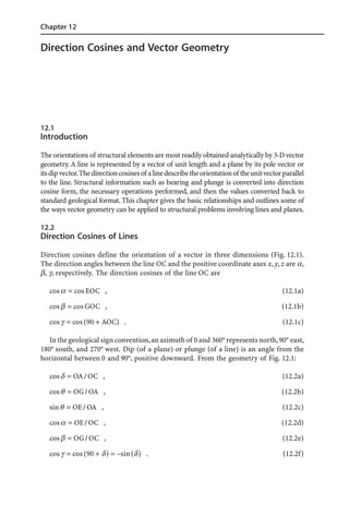
1. Chapter 12
Direction Cosines and Vector Geometry
12.1
Introduction
The orientations of structural elements are most readily obtained analytically by 3-D vector
geometry. A line is represented by a vector of unit length and a plane by its pole vector or
its dip vector. The direction cosines of a line describe the orientation of the unit vector parallel
to the line. Structural information such as bearing and plunge is converted into direction
cosine form, the necessary operations performed, and then the values converted back to
standard geological format. This chapter gives the basic relationships and outlines some of
the ways vector geometry can be applied to structural problems involving lines and planes.
12.2
Direction Cosines of Lines
Direction cosines define the orientation of a vector in three dimensions (Fig. 12.1).
The direction angles between the line OC and the positive coordinate axes x, y, z are α ,
β , γ , respectively. The direction cosines of the line OC are
cos α = cos EOC , (12.1a)
cos β = cos GOC , (12.1b)
cos γ = cos (90 + AOC) . (12.1c)
In the geological sign convention, an azimuth of 0 and 360° represents north, 90° east,
180° south, and 270° west. Dip (of a plane) or plunge (of a line) is an angle from the
horizontal between 0 and 90°, positive downward. From the geometry of Fig. 12.1:
cos δ = OA / OC , (12.2a)
cos θ = OG / OA , (12.2b)
sin θ = OE / OA , (12.2c)
cos α = OE / OC , (12.2d)
cos β = OG / OC , (12.2e)
cos γ = cos (90 + δ ) = –sin (δ ) . (12.2f)

2. 374 Chapter 12 · Direction Cosines and Vector Geometry
Fig. 12.1.
Orientation of vector OC in
right-handed xyz space; θ is
the azimuth of the vector and
δ is the plunge. The direction
angles are α , β , γ
12.2.1
Direction Cosines of a Line from Azimuth and Plunge
The direction cosines of a line in terms of its azimuth and plunge are obtained from
the relationships in Eq. 12.2:
cos δ sin θ = (OA / OC) (OE / OA) = OE / OC = cos α , (12.3a)
cos δ cos θ = (OA / OC) (OG / OA) = OG / OC = cos β , (12.3b)
–sin δ = cos γ . (12.3c)
12.2.2
Azimuth and Plunge from Direction Cosines
To reverse the procedure and find the azimuth and plunge of a line from its direction
cosines, divide Eq. 12.3a by 12.3b and solve for θ , then solve Eq. 12.3c for δ :
θ ' = arctan (cos α / cos β ) , (12.4)
δ = arcsin (–cos γ ) . (12.5)
The value θ ' returned by Eq. 12.4 will be in the range of ±90° and must be corrected
to give the true azimuth over the range of 0 to 360°. The true azimuth, θ , of the line can
be determined from the signs of cos α and cos β (Table 12.1). The direction cosines
give a directed vector. The vector so determined might point upward. If it is necessary
to reverse its sense of direction, reverse the sign of all three direction cosines. Note that
division by zero in Eq. 12.4 must be prevented.
An Excel equation that returns the azimuth in the correct quadrant has the form
=IF(cell B<=0,180+Cell E,IF(cell A>=0,cell E,360+cell E)) (12.6)
where cell A contains cos α , cell B contains cos β , and cell E contains Eq. 12.4.

3. 12.2 · Direction Cosines of Lines 375
Table 12.1.
Relationship between signs
of the direction cosines and
the quadrant of the azimuth
of a line
12.2.3
Direction Cosines of a Line on a Map
The direction cosines of a line defined by its horizontal, h, and vertical, v, dimensions
on a map can be found by letting δ = arctan (v / h) in Eqs. 12.3:
cos α = cos (arctan (v / h)) sin θ , (12.7a)
cos β = cos (arctan (v / h)) cos θ , (12.7b)
cos γ = –sin (arctan (v / h)) . (12.7c)
Both v and h are taken as positive numbers in Eqs. 12.7 and the resulting dip is
positive downward.
The direction cosines of a line defined by the xyz coordinates of its two end points
are obtained by letting point 1 be at O and point 2 be at C in Fig. 12.1. Then
x2 – x1 = OE , (12.8a)
y2 – y1 = OG , (12.8b)
z2 – z1 = AC . (12.8c)
Substitute Eqs. 12.8 into 12.3 to obtain
cos α = (x2 – x1) / OC , (12.9a)
cos β = (y2 – y1) / OC , (12.9b)
cos γ = –sin δ = –AC / OC = –(z2 – z1) / OC = (z1 – z2) / OC , (12.9c)
where OC = L, given by
L = [(x2 – x1)2 + (y2 – y1)2 + (z2 – z1)2]1/2 . (12.10)
Using the convention that point 1 is higher and point 2 is lower, a downward-di-
rected bearing is positive in sign.

4. 376 Chapter 12 · Direction Cosines and Vector Geometry
12.2.4
Azimuth and Plunge of a Line from the End Points
To find the azimuth and plunge of a line from the coordinates of two points, substitute
Eq. 12.9 into 12.4 and 12.5:
θ ' = arctan ((x2 – x1) / (y2 – y1)) , (12.11)
δ = arcsin ((z2 – z1) / L) . (12.12)
The value of L is given by Eq. 12.10. If y2 = y1, there is a division by zero in Eq. 12.13
which must be prevented. The value of θ is obtained from Table 12.1.
12.2.5
Pole to a Plane
The pole to a plane defined by its dip vector has the same azimuth as the dip vector,
and a plunge of δ p = δ + 90. Substitute this into Eqs. 12.3 to obtain the direction co-
sines of the pole, p, in terms of the azimuth, θ , and plunge, δ , of the bedding dip:
cos α p = cos (δ + 90) sin θ = –sin δ sin θ , (12.13a)
cos β p = cos (δ + 90) cos θ = –sin δ cos θ , (12.13b)
cos γ p = –sin (δ + 90) = –cos δ . (12.13c)
12.3
Attitude of a Plane from Three Points
The general equation of a plane (Foley and Van Dam 1983) is
Ax + By + Cz + D = 0 . (12.14)
The equation of the plane from the xyz coordinates of three points is
. (12.15)
This expression is expanded by cofactors to find the coefficients A, B, C, and D:
A = y1 z2 + z1 y3 + y2 z3 – z2 y3 – z3 y1 – z1 y2 , (12.16a)
B = z2 x3 + z3 x1 + z1 x2 – x1 z2 – z1 x3 – x2 z3 , (12.16b)

5. 12.4 · Vector Geometry of Lines and Planes 377
C = x1 y2 + y1 x3 + x2 y3 – y2 x3 – y3 x1 – y1 x2 , (12.16c)
D = z1 y2 x3 + z2 y3 x1 + z3 y1 x2 – x1 y2 z3 – y1 z2 x3 – z1 x2 y3 . (12.16d)
The direction cosines of the pole to this plane are (Eves 1984)
cos α p = A / E , (12.17a)
cos β p = B / E , (12.17b)
cos γ p = C / E , (12.17c)
where
E = (A2 + B2 + C2)1/2 , (12.18)
and the sign of E = –sign D if D ≠ 0; = sign C if D = 0 and C ≠ 0; = sign B if C = D = 0.
The direction cosines of the pole may be converted to the direction cosines of the
dip vector. If cos γ p is negative, the pole points downward. Reverse the signs on all
three direction cosines to obtain the upward direction. If cos γ p is positive, the pole
points upward, and the dip azimuth is the same as that of the pole and the dip amount
is equal to 90° plus the angle between the pole and the z axis:
cos α = A / E , (12.19a)
cos β = B / E , (12.19b)
cos γ = cos (90 + arccos (C / E)) . (12.19c)
To find the azimuth and plunge of the dip direction, use Eqs. 12.4 and 12.5 and
Table 12.1 or the Excel equation 12.6.
12.4
Vector Geometry of Lines and Planes
Vector geometry (Thomas 1960) is an efficient method for the analytical computation
of the relationships between lines and planes. A 3-D vector has the form
v = li + mj + nk , (12.20)
where i, j, k = unit vectors parallel to the x, y, z axes, respectively (Fig. 12.2) and the
coefficients are the direction cosines l, m, n of the line with respect to the correspond-
ing axes. The vector v is a unit vector if its length is equal to one, and gives the orien-
tation of a line. The length of the vector is
|li + mj + nk| = (l2 + m2 + n2)1/2 , (12.21)

6. 378 Chapter 12 · Direction Cosines and Vector Geometry
Fig. 12.2.
Vector components in the
xyz coordinate system. Vector
components i, j, k each have
lengths equal to one
where the vertical bars = the absolute value of the expression between them. The di-
rection cosines of any vector can be normalized to generate a unit vector by dividing
each direction cosine (l, m, and n) by the right-hand side of Eq. 12.21.
12.4.1
Angle between Two Lines or Planes
The angle, Θ , between two lines, is given by the scalar or dot product of the two unit
vectors with the same orientations as the lines. If the two vectors represent the poles
to planes or the dip vectors of planes, then the dot product is the angle between the
planes, normal to their line of intersection (Fig. 12.3). The dot product is defined as
v1 · v2 = |v1| |v2| cos Θ , (12.22)
where |v| = 1 for a unit vector and v1 · v2 is evaluated as
v1 · v2 = l1 l2 + m1 m2 + n1 n2 , (12.23)
where the subscript “1” = the direction cosines of the first vector and subscript “2” = the
direction cosines of the second vector. Equating 12.22 and 12.23 gives the angle be-
tween two unit vectors:
cos Θ = l1 l2 + m1 m2 + n1 n2 . (12.24)
12.4.2
Line Perpendicular to Two Vectors
The orientation of a line perpendicular to two other vectors is given by the vector prod-
uct, also called the cross product (Fig. 12.3). The cross product of two vectors is defined as
v1 × v2 = n |v1| |v2| sin Θ , (12.25)
where n = a unit vector perpendicular to the plane of v1 and v2. When the vectors are
unit vectors given in terms of the direction cosines, the cross product is:

7. 12.4 · Vector Geometry of Lines and Planes 379
Fig. 12.3.
Geometry of the dot product
and cross product. Θ is the
angle between v1 and v2; v3 is
perpendicular to the plane
of v1 and v2. The shaded plane
is perpendicular to v1 and
the ruled plane is perpen-
dicular to v2
. (12.26)
In Eq. 12.26, v3 is the vector perpendicular to both v1 and v2. The order of mul-
tiplication changes the direction of v3 but not the orientation of the line or its mag-
nitude.
12.4.3
Line of Intersection between Two Planes
The properties of the cross product make it suitable for solving a number of problems
in structural analysis. For example, two dip domains can be defined by their poles (or
their dip vectors) and the cross product of these vectors will give the orientation of the
hinge line between them. If the pole to a plane is defined by the azimuth (θ ) and dip (δ )
of a vector pointing in the dip direction, the orientation of this vector in terms of di-
rection cosines is given by Eqs. 12.13, which are
l = cos α p = –sin δ sin θ , (12.27a)
m = cos β p = –sin δ cos θ , (12.27b)
n = cos γ p = –cos δ . (12.27c)
The subscript “p” = the pole to a plane. Let the subscript “1” = the first do-
main dip, 2 = the second domain dip, and h = the hinge line, then substitute Eqs. 12.27
into 12.26 to obtain a vector parallel to the hinge line in terms of the direction co-
sines:
cos α = sin δ 1 cos θ 1 cos δ 2 – cos δ 1 sin δ 2 cos θ 2 , (12.28a)
cos β = cos δ 1 sin δ 2 sin θ 2 – sin δ 1 sin θ 1 cos δ 2 , (12.28b)
cos γ = sin δ 1 sin θ 1 sin δ 2 cos θ 2 – sin δ 1 cos θ 1 sin δ 2 sin θ 2 . (12.28c)

8. 380 Chapter 12 · Direction Cosines and Vector Geometry
The direction cosines must be normalized to ensure that the sum of their squares
equals 1, which is done by dividing through by Nc where
Nc = (cos α 2 + cos β 2 + cos γ 2)1/2 . (12.29)
The final equation for the line of intersection between two planes is
cos α h = (cos α ) / Nc , (12.30a)
cos β h = (cos β ) / Nc , (12.30b)
cos γ h = (cos γ ) / Nc . (12.30c)
The azimuth and dip of the line of intersection are given by Eqs. 12.4, 12.5 and Table 12.1.
12.4.4
Plane Bisecting Two Planes
The axial surface of a constant thickness fold hinge is a plane that bisects the angle be-
tween the two adjacent bedding planes and can be found as a vector sum. A vector sum
is the diagonal of the parallelogram formed by two vectors. If the two vectors forming the
sum have the same lengths, as do unit vectors, then the diagonal bisects the angle between
them (Fig. 12.4). The sum of two vectors is the sum of their corresponding components:
v1 + v2 = (l1 + l2)i + (m1 + m2)j + (n1 + n2)k . (12.31)
The unit vector that bisects the angle between the two vectors v1 and v2 is
v3 = (1 / Nb)(l1 + l2)i + (1 / Nb)(m1 + m2)j + (1 / Nb)(n1 + n2)k , (12.32)
where
Nb = ((l1 + l2)2 + (m1 + m2)2 + (n1 + n2)2)1/2 (12.33)
serves to normalize the length to make the resultant a unit vector. Depending on the
directions of v1 and v2, this vector could bisect either the acute angle or the obtuse
Fig. 12.4.
Bisecting vector (b) of the
angle between two vectors in
the plane of the two vectors

9. 12.4 · Vector Geometry of Lines and Planes 381
angle. If the two vectors are the poles to planes, the vector bisector is the pole to one
of the two bisecting planes. The two bisecting planes are separated by 90°.
To bisect a given pair of planes, begin with the poles of the planes to be bisected
(Eqs. 12.27). Substitute Eqs. 12.27 for both planes into 12.32 and use the same
subscripting convention as above, with the subscript “B” = bisector, to obtain
cos α B1 = –(1 / NB)(sin δ 1 sin θ 1 + sin δ 2 sin θ 2) , (12.34a)
cos β B1 = –(1 / NB)(sin δ 1 cos θ 1 + sin δ 2 cos θ 2) , (12.34b)
cos γ B1 = –(1 / NB)(cos δ 1 + cos δ 2) , (12.34c)
where, from Eq. 12.33:
NB = [(cos δ 1 sin θ 1 + cos δ 2 sin θ 2)2 + (sin δ 1 cos θ 1 + sin δ 2 cos θ 2)2
+ (cos δ 1 + cos δ 2)2]1/2 . (12.35)
Equations 12.34 and 12.35 give the pole to one of the bisecting planes. The direction
cosines of the pole should be converted to the dip vector. If cos γ B1 is negative, the pole
points downward. Reverse the signs on all three direction cosines to obtain the upward
direction. If cos γ B1 is positive, the pole points upward, and the dip azimuth is the same
as that of the pole and the dip amount is equal to 90° plus the angle between the pole
and the z axis:
cos α 1 = cos α B1 , (12.36a)
cos β 1 = cos β B1 , (12.36b)
cos γ 1 = cos (90 + arccos (cos γ B1)) . (12.36c)
The procedure given above finds one of the two bisectors of the two planes. The
other bisecting plane includes the line normal to both the line of intersection of the
two planes (hinge line, Eqs. 12.30) and to the first bisecting line (Eqs. 12.36). Find the
pole to the second plane by substituting Eqs. 12.30 and 12.36 into the cross product
12.26 to obtain
cos α b2 = (1 / Np)(cos β h cos γ B1 – cos γ h cos β B1) , (12.37a)
cos β b2 = (1 / Np)(cos γ h cos α B1 – cos α h cos γ B1) , (12.37b)
cos γ b2 = (1 / Np)(cos α h cos β B1 – cos β h cos α B1) , (12.37c)
where
Np = [(cos β h cos γ B1 – cos γ h cos β B1)2 + (cos γ h cos α B1 – cos α h cos γ B1)2
+ (cos α h cos β B1 – cos β h cos α B1)2]1/2 + 1 . (12.38)

10. 382 Chapter 12 · Direction Cosines and Vector Geometry
Fig. 12.5.
Geometry of conjugate faults.
δ i: Dip vectors of fault planes;
σ i: principal stress directions
Equation 12.38 serves as a check on the calculation: it should always equal 1 because
the starting vectors are orthogonal and of unit length. Convert this pole to the bisect-
ing plane (Eqs. 12.37) into the dip vector of the plane as done above. First reverse the
direction of the vector if it points downward (cos γ negative) by reversing the signs of
all the direction cosines. Then
cos α 2 = cos α b2 , (12.39a)
cos β 2 = cos β b2 , (12.39b)
cos γ 2 = cos (90 + arccos (cos γ b2)) . (12.39c)
The azimuth and dip of the planes in Eqs. 12.36 and 12.39 are given by Eqs. 12.4,
12.5 and Table 12.1.
If the two planes being bisected are conjugate faults (Fig. 12.5), then the line of in-
tersection of the faults is the intermediate principal compressive stress axis (σ 2), the
line that bisects the acute angle is the maximum principal compressive stress axis (σ 1),
and the line that bisects the obtuse angle is the least principal compressive stress
axis (σ 3).