1. 1 OF 21
3. OPTIMIZATION
3.1 BACKGROUND
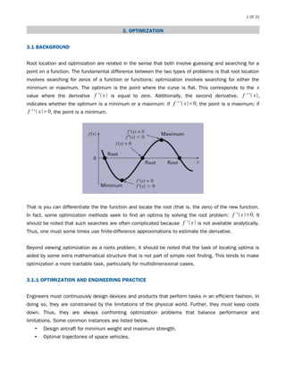
Root location and optimization are related in the sense that both involve guessing and searching for a
point on a function. The fundamental difference between the two types of problems is that root location
involves searching for zeros of a function or functions; optimization involves searching for either the
minimum or maximum. The optimum is the point where the curve is flat. This corresponds to the x
value where the derivative f ' x is equal to zero. Additionally, the second derivative, f ' '  x,
indicates whether the optimum is a minimum or a maximum: if f ' '  x0, the point is a maximum; if
f ' '  x0, the point is a minimum.
That is you can differentiate the the function and locate the root (that is, the zero) of the new function.
In fact, some optimization methods seek to find an optima by solving the root problem: f ' x=0. It
should be noted that such searches are often complicated because f ' x is not available analytically.
Thus, one must some times use finite-difference approximations to estimate the derivative.
Beyond viewing optimization as a roots problem, it should be noted that the task of locating optima is
aided by some extra mathematical structure that is not part of simple root finding. This tends to make
optimization a more tractable task, particularly for multidimensional cases.
3.1.1 OPTIMIZATION AND ENGINEERING PRACTICE
Engineers must continuously design devices and products that perform tasks in an efficient fashion. In
doing so, they are constrained by the limitations of the physical world. Further, they must keep costs
down. Thus, they are always confronting optimization problems that balance performance and
limitations. Some common instances are listed below.
• Design aircraft for minimum weight and maximum strength.
• Optimal trajectories of space vehicles.

2. 2 OF 21
• Design civil engineering structures for minimum cost.
• Design water-resource projects to mitigate flood damage while yield maximum hydropower.
• Predict structural behaviour by minimizing potential energy.
• Material-cutting strategy for minimum cost.
• Design pump and heat transfer equipment for maximum efficiency.
• Maximize power output of electrical networks and machinery while minimizing heat generation.
• Optimal planning and scheduling.
• Statistical analysis and models with minimum error.
• Optimal pipeline networks.
• Inventory control.
• Maintenance planning to minimize cost.
• Minimize waiting and idling times.
• Design waste treatment systems to meet water-quality standards at least cost.
3.1.2 MATHEMATICAL BACKGROUND
An optimization or mathematical programming problem generally can be stated as:
Minimize f x
Subject to gi x≤0 i=1,2,... ,m
hix=0 i=1,2,... , p
where x is an n-dimensional design vector, f x is the objective function, gi x≤0 are inequality
constraints, hix=0 are equality constraints.
The process of finding a maximum versus finding a minimum is essentially identical because the same
value, x*, both minimizes f(x) and maximize -f(x). This equivalence is illustrated graphically for a one-
dimensional function below.

3. 3 OF 21
3.2 ONE-DIMENSIONAL UNCONSTRAINED OPTIMIZATION
In the root location, several roots can occur for a single function. Similarly, both local and global optima
can occur in optimization. In almost all instances, we will be interested in finding the absolute highest
or lowest value of a function. Thus, we must take care that we do not mistake a local result for the
global optimum.
Distinguishing a global from a local extremum can be very difficult problem for the general case. There
are there useful ways to approach this problem. First, insight into the behaviour of low-one dimensional
functions can some times be obtained graphically. Second, finding optima based on widely varying and
perhaps randomly generated starting guesses, and then selecting the largest of these as global.
Finally, perturbing the starting point associated with a local optimum and seeing if the routine returns a
better point or always returns to the same point. Although all these approaches can be utility, the fact
is that in some problems (usually the large ones), there may be no practical way to ensure that you
have located a global optimum. However, although you should always be sensitive to the issue, it is
fortunate that there are numerous engineering problems where you can locate the global optimum in an
unambiguous fashion.
3.2.1 GOLDEN-SECTION SEARCH
In solving for the root of a single nonlinear equation, the goal was to find the value of variable x that
yields a zero of the function f x. Single-variable optimization has the goal of finding the value of x
that yields an extremum, either a maximum or minimum of f x.
The golden-section search is simple and similar to the bisection approach for locating roots. For
simplicity, we will focus on the problem of finding a maximum.

4. 4 OF 21
L0=L1L2 or
L1
L0
=
L2
L1
L1
L1L2
=
L2
L1
1
1
L2
L1
=
L2
L1
Given R=
L2
L1
1
1R
=R
R2
R−1=0
Solve for R
R=
−11−41−1
2
=
5−1
2
ALGORITHM
Step 1: Select the two initial guesses, xL and xU, that bracket one local extremum of f x.
Step 2: Two interior points x1 and x2 are chosen according to the golden ratio.
d=
5−1
2
xU −xL
x1=xLd
x2=xU −d
Step 3: Evaluate the function at these two interior points x1 and x2.
If f x1 f x2, then xL=x2 ==> [ x2, xU ]
If f  x2 f  x1, then xU =x1 ==> [ xL , x1]

5. 5 OF 21
As the iterations are repeated, the interval containing the extremum is reduced rapidly. In fact, each
round the interval is reduced by a factor of the golden ratio. This is not quite as good as the reduction
achieved with bisection, but this is a harder problem.
Ea=1−R
∣xu−xL
xopt
∣100
EXAMPLE 1 Use the golden-section search to find the maximum of
f x=2sin x−
x2
10
within the interval xL=0 and xU =4.
-6.0 -4.0 -2.0 0.0 2.0 4.0 6.0 8.0 10.0
-8.00
-6.00
-4.00
-2.00
0.00
2.00
4.00
f(x)
Iter xL xU f(xL) f(xU) d x1 x2 f(x1) f(x2)
0 0 4 0 -3.1136 2.4721 2.4721 1.5279 0.6300 1.7647
1 0 2.4721 0 0.6300 1.5279 1.5279 0.9443 1.7647 1.5310
2 0.9443 2.4721 1.5310 0.6300 0.9443 1.8885 1.5279 1.5432 1.7647
3 0.9443 1.8885 1.5310 1.5432 0.5836 1.5279 1.3050 1.7647 1.7595
4 1.3050 1.8885 1.7595 1.5432 0.3607 1.6656 1.5279 1.7136 1.7647
5 1.3050 1.6656 1.7595 1.7136 0.2229 1.5279 1.4427 1.7647 1.7755
6 1.3050 1.5279 1.7595 1.7647 0.1378 1.4427 1.3901 1.7755 1.7742
7 1.3901 1.5279 1.7742 1.7647 0.0851 1.4752 1.4427 1.7732 1.7755
8 1.3901 1.4752 1.7742 1.7732 0.0526 1.4427 1.4226 1.7755 1.7757
9 1.3901 1.4427 1.7742 1.7755 0.0325 1.4226 1.4102 1.7757 1.7754
10 1.4102 1.4427 1.7754 1.7755 0.0201 1.4303 1.4226 1.7757 1.7757

6. 6 OF 21
-6.0 -4.0 -2.0 0.0 2.0 4.0 6.0 8.0 10.0
-8.00
-6.00
-4.00
-2.00
0.00
2.00
4.00
f(x)
3.2.2 PARABOLIC INTERPOLATION
Parabolic interpolation takes advantage of the fact that a second-order polynomial often provides a
good approximation to the shape of f x near an optimum.
Just as there is only one straight line connecting two points, there is only one quadratic polynomial or
parabola connecting three points. Thus, if we have three points that jointly bracket an optimum, we can
find a parabola to the points. Then we can differentiate it, set the result equal to zero, and solve for an
estimate of the optimal x. It can be shown through some algebraic manipulations that the result is
x3=
f x0x1
2
−x2
2
 f x1 x2
2
−x0
2
 f  x2x0
2
−x1
2

2 f x0 x1−x22 f x1x2−x02 f x2x0−x1
where x0, x1, and x2 are the initial guesses, and x3 is the value of x that corresponds to the maximum
value of the parabolic fit to the guesses.

7. 7 OF 21
After generating the new point, x3, which is similar to the secant method, is to merely assign the new
points sequentially.
EXAMPLE 2 Use parabolic interpolation to approximate the maximum of
f x=2sin x−
x2
10
with initial guess of x0=0, x1=1, and x2=4.
Iter x0 fx0 x1 fx1 x2 fx2 x3 fx3
1 0 0 1 1.582942 4 -3.113605 1.505535 1.769079
2 1 1.582942 1.505535 1.769079 4 -3.113605 1.490253 1.771431
3 1 1.582942 1.490253 1.771431 1.505535 1.769079 1.425636 1.775722
4 1 1.582942 1.425636 1.775722 1.490253 1.771431 1.426602 1.775725
5 1.425636 1.775722 1.426602 1.775725 1.490253 1.771431 1.427548 1.775726
6 1.426602 1.775725 1.427548 1.775726 1.490253 1.771431 1.427551 1.775726
7 1.427548 1.775726 1.427551 1.775726 1.490253 1.771431 1.427552 1.775726
8 1.427551 1.775726 1.427552 1.775726 1.490253 1.771431 1.427552 1.775726
0 1 2 3 4 5 6 7 8 9
1.380000
1.400000
1.420000
1.440000
1.460000
1.480000
1.500000
1.520000
x3
3.2.3 NEWTON'S METHOD
Recall that the Newton-Raphson method is an open method that finds the root x of a function such that
f x=0. The method is summarized as:
xi1=xi−
f  xi
f ' xi
A similar open approach can be used to fine an optimum of f x by defining a new function,
g x= f '  x. Thus, because the same optimal value x * satisfies both f ' x
*
=gx
*
=0, we can use
the following method as a technique to find the minimum or maximum of f x.
xi1=xi−
f ' xi
f ' '  xi 

8. 8 OF 21
EXAMPLE 3 Use Newton's method to find the maximum of
f x=2sin x−
x2
10
with initial guess of x0=2.5.
f ' x=2cos x−
x
5
f ' '  x=−2sin x−
1
5
Iter x fx f'(x) f''(x)
0 2.5 1 -2.10229 -1.39694
1 0.995082 2 0.889853 -1.87761
2 1.469011 2 -0.09058 -2.18965
3 1.427642 2 -0.00020 -2.17954
4 1.427552 2 -0.00000 -2.17952
5 1.427552 2 0 -2.17952
0 1 2 3 4 5 6
0
0.5
1
1.5
2
2.5
3
x
Although Newton's method works well in some cases, it is impractical for cases where the derivatives
cannot be conveniently evaluated. For these cases, other approaches that do not involve derivative
evaluation are available. For example, a secant-like Newton's method can be developed by using finite
difference approximations for the derivative evaluation.

9. 9 OF 21
3.3 MULTIDIMENSIONAL UNCONSTRAINED OPTIMIZATION
Techniques for multidimensional unconstrained optimization can be classified in a number of ways. The
approaches that do not require derivative evaluation are called non-gradient or direct methods. Those
that require derivatives are called gradient methods.
3.3.1 DIRECT METHODS
These methods vary from simple brute force approaches to more elegant techniques that attempt to
exploit the nature of the function.
3.3.1.1 RANDOM SEARCH
As the name implies, this method repeatedly evaluates the function at randomly selected values of the
independent variables. If a sufficient number of samples are conducted, the optimum will eventually be
located.
Random number generators typically generate values between 0 and 1. If we designate such a number
as rx, the following formula can be used to generate x values randomly within a range between xL and
xU.
x=xLxU −xLrx
Similarly for y, a formula can be used to generate y values randomly within a range between yL and yU
as follows.
y=yL yU −yLry

10. 10 OF 21
EXAMPLE 4 Use a random number generator to locate the maximum of
f x , y=y−x−2 x2
−2 x y−y2
in the domain bounded by x = –2 to 2 and y = 1 to 3.
Iter rx xL xU x ry yL yU y f(x,y) Max f(x,y)
0 0.457177 -2 2 -0.17129 0.724690 1 3 2.449380 -2.59836 -2.59836
1 0.580900 -2 2 0.323598 0.644624 1 3 2.289247 -4.96603 -2.59836
2 0.676533 -2 2 0.706134 0.103299 1 3 1.206599 -3.65670 -2.59836
3 0.067229 -2 2 -1.73109 0.012434 1 3 1.024868 -0.73945 -0.73945
4 0.073551 -2 2 -1.70579 0.330744 1 3 1.661488 0.455584 0.455584
5 0.761418 -2 2 1.045673 0.576060 1 3 2.152120 -10.2129 0.455584
397 0.720023 -2 2 0.880092 0.791837 1 3 2.583673 -11.0687 1.249151
398 0.054367 -2 2 -1.78253 0.519305 1 3 2.038610 0.578147 1.249151
399 0.269250 -2 2 -0.92300 0.559340 1 3 2.118679 0.760100 1.249151
400 0.274284 -2 2 -0.90287 0.330417 1 3 1.660833 1.174018 1.249151
0 50 100 150 200 250 300 350 400 450
-12
-10
-8
-6
-4
-2
0
2
f(x,y)
This simple brute force approach works even for discontinuous and non-differentiable functions.
Furthermore, it always finds the global optimum rather than a local optimum. It major shortcoming is
that as the number of independent variables grows, the implementation effort required can become
onerous. In addition, it is not efficient because it takes no account of the behaviour into account as
well as the results of previous trials to improve the speed of convergence.

11. 11 OF 21
3.3.2 GRADIENT METHODS
As the name implies, gradient methods explicitly use derivative information to generate efficient
algorithm to locate optima.
The first derivative of a one-dimensional function provides a slope or tangent to the function being
differentiated. For the standpoint of optimization, this is useful information. For example, if the slope is
positive, it tells us that increasing the independent variable will lead to a higher value of the function
we are exploring. The first derivative, thus, may tell us when we have reached an optimal value since
this is the point that the derivative goes to zero. Furthermore, the sign of the second derivative can tell
us whether we have reached a minimum (positive second derivative) or a maximum (negative second
derivative).
To fully understand multidimensional searches, we must first understand how the first and second
derivatives are expressed in a multidimensional context.
THE GRADIENT If we are interested in gaining evaluation as quickly as possible, the gradient tells us
what direction to move locally and how much we will gain by taking it.
 f x =
{
∂ f  x
∂ x1
∂ f  x
∂ x2
⋮
∂ f  x
∂ xn
}
THE HESSIAN For one-dimensional problems, both the first and second derivatives provide valuable
information for searching out optima. The first derivative provides a steepest trajectory of the function
and tells us that we have reached an optimum. Once at an optimum, the second derivative tells us
whether we are a maximum (negative f ' '  x) or a minimum (positive f ' '  x).
You might expect that if the partial second-order derivatives with respect to both x and y are both
negative, then you reached a maximum. In fact, whether a maximum or a minimum occurs involves not
only the partials with respect to x and y but also the second partial with respect to x and y. Assuming
that the partial derivatives are continuous at near the point being evaluated, the following quantity can
be computed:
∣H∣=
∂
2
f
∂
2
x
2
∂
2
f
∂ y
2
–
∂
2
f
∂ x ∂ y

2

12. 12 OF 21
Three cases can occur
• If ∣H∣0 and ∂2
f /∂ x2
0, then f x , y has a local minimum.
• If ∣H∣0 and ∂2
f /∂ x2
0, then f x , y has a local maximum.
• If ∣H∣0, then f x , y has a saddle point.
The quantity ∣H∣ is equal to the determinant of a matrix made up of the second derivatives.
H =
[
∂2
f
∂ x
2
∂2
f
∂ x ∂ y
∂2
f
∂ y ∂ x
∂2
f
∂ y
2 ]
where this matrix is formally referred to as the Hessian of f.
FINITE-DIFFERENCE APPROXIMATIONS It should be mentioned that, for cases where they are
difficulty or inconvenient to compute analytically, both the gradient and Hessian can be evaluated
numerically. That is, the independent variables can be perturbed slightly to generate the required
partial derivatives.
∂ f
∂ x
=
f x x , y− f  x− x , y
2 x
∂ f
∂ y
=
f x , y y− f x , y− y
2 y
∂2
f
∂ x
2
=
f x x , y−2f x , y f x− x , y
2 x
2
∂2
f
∂ y
2
=
f x , y y−2f  x , y f x , y− y
2 y
2
∂2
f
∂ x∂ y
=
f x x , y y− f x x , y− y− f x− x , y y f x− x , y− y
4 x  y
where  is some small fractional value.

13. 13 OF 21
3.3.2.1 STEEPEST ASCENT/DESCENT METHOD
An obvious strategy for climbing a hill would be to determine the maximum slope that your stating
position and then start walking in that direction. However, unless you are lucky and started on a ride
that pointed directly to the summit, as soon as you moved, your path would diverge from the steepest
ascent direction.
Starting at x0 and y0, the coordinates of any point in the gradient direction can be expressed as
x=x0
∂ f
∂ x
h
y= y0
∂ f
∂ y
h
where h is distance along the h axis.
Then we can convert a two-dimensional function of x and y into one-dimensional function in h. The
optimum h* is the value of the step that maximizes f h and hence f x , y in the gradient direction.
This problem is equivalent to finding the maximum of a function of a single variable h. This method is
called steepest ascent where an arbitrary step size h is used.
EXAMPLE 5 Use the steepest ascent to locate the maximum of
f  x , y=2 x y2 x−x
2
−2 y
2
using initial guesses, x=−1 and y=1.
 f =
{2 y2−2 x
2 x−4 y }
At x=−1 and y=1
x=−16h
y=1−6h
Thus
f h=−180 h2
72 h−7
Use optimum step size h
*
=0.2.

14. 14 OF 21
Iter x y dfdx dfdy f(x,y) h*
0 -1.0000 1.0000 6.0000 -6.0000 -7.0000 0.2
1 0.2000 -0.2000 1.2000 1.2000 0.2000 0.2
2 0.4400 0.0400 1.2000 0.7200 0.7184 0.2
3 0.6800 0.1840 1.0080 0.6240 1.0801 0.2
4 0.8816 0.3088 0.8544 0.5280 1.3397 0.2
5 1.0525 0.4144 0.7238 0.4474 1.5261 0.2
63 1.9999 1.0000 0.0000 0.0000 2.0000 0.2
64 1.9999 1.0000 0.0000 0.0000 2.0000 0.2
65 2.0000 1.0000 0.0000 0.0000 2.0000 0.2
66 2.0000 1.0000 0.0000 0.0000 2.0000 0.2
0 5 10 15 20 25 30 35 40 45
-8.0000
-6.0000
-4.0000
-2.0000
0.0000
2.0000
4.0000
f(x,y)
The second derivative can be used to evaluate the optimum as shown.
H = [−2 2
2 −4]
∣H∣=40
Therefore f 2,1=2 is a maximum.

15. 15 OF 21
3.3.2.1 NEWTON'S METHOD
Newton's method for a single variable can be extended to multi-variable cases. Write a second-order
Taylor series for f  x near x=xi,
f  x= f xi f
T
x−xi
1
2
x−xi
T
H i x−xi
At the minimum,
∂ f  x
∂ x j
=0 for j=1,2,...,n
Thus
 f = f  xi H ix−xi=0
If H is nonsingular,
xi1=xi−H i
−1
 f
which can be shown to converge quadratically near the optimum. This method again performs better
than the steepest ascent method. However, note that the method requires both the computation of
second derivatives and matrix inversion at each iteration. Thus, the method is not very useful in
practice for functions with large numbers of variables. Furthermore, Newton's method may not
converge if the starting point is not close to the optimum.
EXAMPLE 6 Use the Newton's method to locate the maximum of
f  x , y=2 x y2 x−x
2
−2 y
2
using initial guesses, x=−1 and y=1.
 f ={2 y2−2 x
2 x−4 y }
H = [−2 2
2 −4]
Iter x,y f(x,y) G H inv(H) inv(H)*G
0 -1.00 -7.00 6.00 -2 2 -1.00 -0.50 -3.00
1.00 -6.00 2 -4 -0.50 -0.50 0.00
1 2.00 2.00 0.00 -2 2 -1.00 -0.50 0.00
1.00 0.00 2 -4 -0.50 -0.50 0.00
2 2.00 2.00 0.00 -2 2 -1.00 -0.50 0.00
1.00 0.00 2 -4 -0.50 -0.50 0.00
3 2.00 2.00 0.00 -2 2 -1.00 -0.50 0.00
1.00 0.00 2 -4 -0.50 -0.50 0.00

16. 16 OF 21
0 0.5 1 1.5 2 2.5 3 3.5
-8.00
-6.00
-4.00
-2.00
0.00
2.00
4.00
f(x,y)
3.4 CONSTRAINED OPTIMIZATION
Linear programming (LP) is an optimization approach that deals with meeting a desired objective
function such as maximizing profit or minimizing cost in the presence of constraints such as limited
resources. The term linear connotes that the mathematical functions representing both the objective
and constraints are linear. The term programming does not mean computer programming but rather
connotes scheduling or setting and agenda.
There are a number of approaches for handling nonlinear optimization problems in presence of
constraints. These can generally be divided into indirect and direct approaches. A typical indirect
approach uses so-called penalty functions. These involve placing additional expression to make the
objective function less optimal as the solution approaches a constraint. Thus, the solution will be
discouraged from violating constraints. Although such methods can be useful in some problems, they
can become arduous when the problem involves many constraints.
3.4.1 PENALTY FUNCTION METHOD
We will focus on understanding the necessary conditions for optimality for the constrained problem:
Minimize f  x
Subject to gi x≤0 for i=1,... ,m
hj x=0 for j=1,...,l
3.4.1.1 EXTERIOR PENALTY FUNCTIONS
For the general problem, the quadratic penalty function P x is developed as
P x=∑
i=1
m
{max[0, gi x]}
2
∑
j=1
l
[h jx]
2
.
Now let us define a composite function.
T x = f xr Px

17. 17 OF 21
where r0 is called a penalty parameter. The parameter r controls the degree of penalty for violating the
constraint. The unconstrained optimization T(x), for increasing values of r, results in a sequence of points that
converges to the minimum of x* = 5 from the outside of the feasible region. Since convergence is from the
outside of the feasible region, we call these exterior point methods. The idea is that if x strays too far from the
feasible region, the penalty term ri Px becomes large when ri is large. As ri ∞ the tendency will be to draw
the unconstrained minima towards the feasible region so as to reduce the value of the penalty term. That is, a
large penalty is attached to being infeasible.
PROCEDURE
1. For some r10, find an unconstrained local minimum of T x ,r1. Denote the solution by xr1.
2. Choose r2r1 and using xr1 as a starting guess, minimize T x ,r2. Denote the solution as xr2.
3. Proceed in this fashion, minimizingT x ,ri for a strictly monotonically increasing sequence ri.
To illustrate the concept, consider a simple problem involving only one variable, x.
Minimize f x
Subject to g x≤0
where f x is a monotonically decreasing function of x. We will now define a penalty function.
EXAMPLE 7
Minimize f  x=100/ x
Subject to g x=x−5≤0
T x ,r  = 100/ xr {max [0, x−5]}
2
Choose: r=10
T x ,r  = 100/ x10{max[0, x−5]}
2
= 100/ x10{x−5}
2
Choose: r=5
T x ,r  = 100/ x5{max[0, x−5]}
2
= 100/ x5{x−5}
2
Choose: r=2
T x ,r  = 100/ x2{max [0,x−5]}
2
= 100/ x2{x−5}
2
Choose: r=1
T x ,r  = 100/ x1{max[0, x−5]}
2
= 100/ x1{x−5}
2
The minimum of T for various values of r leads to point xr as given in the following table.

18. 18 OF 21
r x f x* f* g*
1 1 100 6.2713 15.9457 1.2713
10 6.2713 15.9457 5.1859 19.283 0.1859
100 5.1859 19.283 5.0198 19.9209 0.0198
1000 5.0198 19.9209 5.0020 19.9920 0.0020
10000 5.0020 19.9920 5.0020 19.9992 0.0020
100000 5.0020 19.9992 5.0000 19.9999 0.0000
1000000 5.0000 19.9999 5.0000 20.0000 0.0000
3.5 4 4.5 5 5.5 6 6.5
0
5
10
15
20
25
30
35
40
r=10
r=5
r=2
r=1
3.4.1.2 INTERIOR PENALTY FUNCTIONS
In interior point of barrier methods, we approach the optimum from the interior of the feasible region. Only
inequality constraints are permitted in this class of methods. Thus, we consider the feasible region to be defined
by ={x : gi x≤0,i=1,..., m}. Interior penalty functions, Bx, are defined with properties: (I) B is
continuous, (ii) Bx≥0, (iii) Bx ∞ as bold x approaches the boundary of . Two popular choices are:
Inverse Barrier Function: Bx=−∑
i=1
m
1
gix
Log Barrier Function: Bx=−∑
i=1
m
log[−gix]
We should define log −gi=0 when gi x−1 to ensure that B≥0. This is not a problem when constraints
are expressed in normalized from in which case g−1 implies a highly inactive constraint which will not play a
role in determining the optimum.
For instance, we should express the constraint x≤1000 as g=x/1000 –1≤0. The T-function is defined as:
T x ,r = f x
1
r
B x

19. 19 OF 21
Starting from a point x0∈ and r0, the minimum of T will in general provide us with a new point which is in
, since the value of T becomes infinite on the boundary. As r is increased, the weighting of the penalty term is
decreased. This allows further reduction in f  x while maintaining feasibility.
EXAMPLE 8
Minimize f x=2x−62
Subject to g x=x−5≤0
Choose x0=3,r=1
T x ,r = 2x−6
2

1
r
−1
x−5
= 2x−6
2
−
1
1
1
x−5
1/r x f x* f* g*
100 1 50 2.3742 26.2926 -2.6258
10 2.3742 26.2926 3.9071 8.7606 -1.0929
1 3.9071 8.7606 4.5803 4.0309 -0.4197
0.5 4.5803 4.0309 4.6910 3.4271 -0.3090
0.3 4.6910 3.4271 4.7546 3.1020 -0.2454
0.2 4.7546 3.1020 4.7962 2.8982 -0.2038
0.1 4.7962 2.8982 5.0000 2.0000 0.0000
3.5 4 4.5 5 5.5 6 6.5
-25
-20
-15
-10
-5
0
5
10
15
20
25
1/r = 100
1/r = 10
1/r = 1

20. 20 OF 21
3.5 GLOBAL OPTIMUM
3.5.1 PARAMETERIZATION TECHNIQUE
Minimize P x
Let V =Px, thus
˙V =J x ˙x.
˙x=J +
x  ˙V 
Then x* can be obtained from x=∫ ˙x d  or numerical method such as the Runge-Kutta method.
The value ˙V  can be view as a slope of a searching path as shown.
˙V =
Pd  x−Px0
 f −0
where Pd  xf  is the desired value of the objective function P x and can be estimated by
Pd  xf = Px 0

21. 21 OF 21
Example 9 Use the Newton's method and the parameterization technique to find the minimum of
f x=x−1x2x−3x5
starting at x0=4.
f x=x4
3 x3
−15 x2
−19 x30
f ' x=4 x3
9 x2
−30 x−19
f ' '  x=12 x2
18 x−30
-8 -6 -4 -2 0 2 4 6
-100
-50
0
50
100
150
200
250
300
350
f(x)
NEWTON'S METHOD
Iter x f(x) f'(x) f''(x)
0 4 162 261 234
1 2.884615 -8.37494 65.36220 121.7751
2 2.347870 -28.0815 11.94685 78.41161
3 2.195510 -29.0349 0.848812 67.36233
4 2.182909 -29.0403 0.005604 66.47347
5 2.182825 -29.0403 0.000000 66.46753