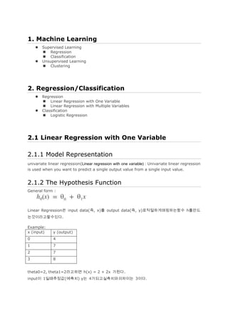
1. 1. Machine Learning
 Supervised Learning
 Regression
 Classification
 Unsupervised Learning
 Clustering
2. Regression/Classification
 Regression
 Linear Regression with One Variable
 Linear Regression with Multiple Variables
 Classification
 Logistic Regression
2.1 Linear Regression with One Variable
2.1.1 Model Representation
univariate linear regression(Linear regression with one variable) : Univariate linear regression
is used when you want to predict a single output value from a single input value.
2.1.2 The Hypothesis Function
General form :
Linear Regression은 input data(즉, x)를 output data(즉, y)로적절하게매핑하는함수 h를만드
는것이라고할수있다.
Example:
x (input) y (output)
0 4
1 7
2 7
3 8
theta0=2, theta1=2라고하면 h(x) = 2 + 2x 가된다.
input이 1일때추정값(예측치) y는 4가되고실측치와의차이는 3이다.

2. 2.1.3 Cost Function
We can measure the accuracy of our hypothesis function by using a cost function. m개의
input data가있을때각 input data에대한예측치 h(x)와실측치 y의평균차이값을최소화하는 theta
가해당 input과 output을가장잘표현하는모델의 parameter가된다.
Cost function은다음과같다.
※ 1/2을곱하는이유는차후계산식에서수학적으로표현이쉽기때문이다.
Cost function을통해얻고자하는 goal은
J()를 theta0과 theta1에대해서그려보면아래와같다.

3. 2.1.4 Gradient Descent
참고 :
- http://personal.ee.surrey.ac.uk/Personal/J.Illingworth/eem.asp/BayenSteepestDesce
ntLecture.pdf
- http://www.evernote.com/shard/s143/sh/c274bc38-2944-4d88-b062-
9f3ded8f8691/55d622f8d2f8a9ae081bbebc50865787
Gradient descent algorithm :
※
2.1.5 Gradient Descent for Linear Regression
편미분부분만전개해보면아래와같고,
frac { partial }{ partial { theta }_{ j } } J({ theta }_{ 0 },{ quad theta }_{ 1 })quad =quad frac { partial }{ partial { theta }_{ j } } frac { 1 }{ 2m } sum
_{ i=1 }^{ m }{ { (h }_{ theta }({ x }^{ (i) }) } quad -quad { y }^{ (i) })^{ 2 } quad quad quad quad quad quad quad quad quad quad quad quad =quad
frac { partial }{ partial { theta }_{ j } } frac { 1 }{ 2m } sum _{ i=1 }^{ m }{ { { (theta }_{ 0 }quad +quad { theta }_{ 1 }x^{ (i) } } } quad -quad
{ y }^{ (i) })^{ 2 }

4. 각 j값에대해서아래와같이쓸수있다.
jquad =quad 0quad :quad frac { partial }{ partial { theta }_{ 0 } } J({ theta }_{ 0 },{ quad theta }_{ 1 })quad =quad frac { 1 }{ m } sum
_{ i=1 }^{ m }{ { (h }_{ theta }({ x }^{ (i) }) } quad -quad { y }^{ (i) }) jquad =quad 1quad :quad frac { partial }{ partial { theta }_{ 1 } }
J({ theta }_{ 0 },{ quad theta }_{ 1 })quad =quad frac { 1 }{ m } sum _{ i=1 }^{ m }{ { (h }_{ theta }({ x }^{ (i) }) } quad -quad { y }^{ (i) })cdot
{ x }^{ (i) }
그러므로위 gradient descent algorithm을각각의 theta에대해다시써보면
repeatquad untilquad convergencequad { qquad { theta }_{ 0 }quad :={ quad theta }_{ 0 }quad -quad alpha frac { 1 }{ m } sum
_{ i=1 }^{ m }{ ({ h }_{ theta }({ x }^{ (i) })-{ y }^{ (i) }) } qquad { theta }_{ 1 }quad :={ quad theta }_{ 1 }quad -quad alpha frac { 1 }{ m } sum
_{ i=1 }^{ m }{ ({ h }_{ theta }({ x }^{ (i) })-{ y }^{ (i) }) } cdot { x }^{ (i) } }
위반복과정을그림으로보기편하게나타내면,
(for fixed , this is a function of x) (function of the parameters )
(https://picasaweb.google.com/104059922827789076358/2011921#576612698120168
1554)

5. 2.1.6 Implementation
- python
from numpy import loadtxt, zeros, ones, array, linspace, logspace
from pylab import scatter, show, title, xlabel, ylabel, plot, contour
#Evaluate the linear regression
defcompute_cost(X, y, theta):
'''
Comput cost for linear regression
'''
#Number of training samples
m = y.size
predictions = X.dot(theta).flatten()
sqErrors = (predictions - y) ** 2
J = (1.0 / (2 * m)) * sqErrors.sum()
return J
defgradient_descent(X, y, theta, alpha, num_iters):
'''
Performs gradient descent to learn theta
by taking num_items gradient steps with learning
rate alpha
'''
m = y.size
J_history = zeros(shape=(num_iters, 1))
for i in range(num_iters):
predictions = X.dot(theta).flatten()
errors_x1 = (predictions - y) * X[:, 0]
errors_x2 = (predictions - y) * X[:, 1]
theta[0][0] = theta[0][0] - alpha * (1.0 / m) * errors_x1.sum()
theta[1][0] = theta[1][0] - alpha * (1.0 / m) * errors_x2.sum()
J_history[i, 0] = compute_cost(X, y, theta)
return theta, J_history
#Load the dataset
data = loadtxt('ex1data1.txt', delimiter=',')
#Plot the data
scatter(data[:, 0], data[:, 1], marker='o', c='b')
title('Profits distribution')
xlabel('Population of City in 10,000s')

6. ylabel('Profit in $10,000s')
#show()
X = data[:, 0]
y = data[:, 1]
#number of training samples
m = y.size
#Add a column of ones to X (interception data)
it = ones(shape=(m, 2))
it[:, 1] = X
#Initialize theta parameters
theta = zeros(shape=(2, 1))
#Some gradient descent settings
iterations = 1500
alpha = 0.01
#compute and display initial cost
print compute_cost(it, y, theta)
theta, J_history = gradient_descent(it, y, theta, alpha, iterations)
print theta
#Predict values for population sizes of 35,000 and 70,000
predict1 = array([1, 3.5]).dot(theta).flatten()
print'For population = 35,000, we predict a profit of %f' % (predict1 *
10000)
predict2 = array([1, 7.0]).dot(theta).flatten()
print'For population = 70,000, we predict a profit of %f' % (predict2 *
10000)
#Plot the results
result = it.dot(theta).flatten()
plot(data[:, 0], result)
show()
#Grid over which we will calculate J
theta0_vals = linspace(-10, 10, 100)
theta1_vals = linspace(-1, 4, 100)
#initialize J_vals to a matrix of 0's
J_vals = zeros(shape=(theta0_vals.size, theta1_vals.size))
#Fill out J_vals
for t1, element in enumerate(theta0_vals):
for t2, element2 in enumerate(theta1_vals):
thetaT = zeros(shape=(2, 1))
thetaT[0][0] = element
thetaT[1][0] = element2
J_vals[t1, t2] = compute_cost(it, y, thetaT)
#Contour plot
J_vals = J_vals.T
#Plot J_vals as 15 contours spaced logarithmically between 0.01 and 100

7. contour(theta0_vals, theta1_vals, J_vals, logspace(-2, 3, 20))
xlabel('theta_0')
ylabel('theta_1')
scatter(theta[0][0], theta[1][0])
show()
※ 출처 :http://aimotion.blogspot.kr/2011/10/machine-learning-with-python-linear.html
- R

8. 2.2 Linear Regression with Multiple Variables
Multiple Features
Linear regression with multiple variables is also known as "multivariate linear
regression."
Size Number of Number of Age of price
bedrooms floors home
x1 X2 X3 X4 y
2104 5 1 45 460
1416 3 2 40 232
1534 3 2 30 315
852 2 1 36 178
… … … … …
nquad =quad left| x^{ (i) } right| ; { (thequad numberquad ofquad features) } x^{ (i) }quad =quad { inputquad featuresquad ofquad thequad i^{ th }quad
trainingquad example } x_{ j }^{ (i) }quad ={ quad valuequad ofquad featurequad jquad inquad thequad i^{ th }quad trainingquad example }
hypothesis function :
h_{ theta }(x)quad =quad theta _{ 0 }quad +quad theta _{ 1 }x_{ 1 }quad +quad theta _{ 2 }x_{ 2 }quad +quad theta _{ 3 }x_{ 3 }quad +quad cdots quad
+quad theta _{ n }x_{ n }
x와 theta를아래와같이나타낼수있으므로
{ xquad =quad left[ begin{ matrix } { x }_{ 0 } { x }_{ 1 } { x }_{ 2 } vdots { x }_{ n } end{ matrix } right] quad in quad { Re }^{ n+1 } },quad
{ theta quad =quad left[ begin{ matrix } { theta }_{ 0 } { theta }_{ 1 } { theta }_{ 2 } vdots { theta }_{ n } end{ matrix } right] quad in quad
{ Re }^{ n+1 } }
위hypothesis function을간단히쓰면,
h_{ theta }(x)quad =quad theta ^{ T }x
Cost function
Parameters :
{ theta }_{ 0 },{ quad theta }_{ 1 },quad ...quad ,{ quad theta }_{ n }quad longrightarrow quad theta
Cost function :

9. J({ theta }_{ 0 },{ theta }_{ 1 },...,{ theta }_{ n })quad =quad frac { 1 }{ 2m } sum _{ i=1 }^{ m }{ { ({ h }_{ theta }({ x }^{ (i) })quad -quad
{ y }^{ (i) }) }^{ 2 } }
Gradient Descent for Multiple Variables
Gradient descent :
repeatquad { qquad { theta }_{ j }quad :=quad { theta }_{ j }quad -quad alpha frac { partial }{ partial { theta }_{ j } }
J({ theta }_{ 0 },{ theta }_{ 1 },...,{ theta }_{ n }) }
Univariate linear regression과multivariate linear regression의 Gradient Descent 구현을비
교해보면아래와같은차이가있는것을알수있다.
repeatquad untilquad convergence:quad lbrace newline qquad theta _{ j }quad :=quad theta _{ j }quad -quad alpha frac { 1 }{ m } sum _{ i=1 }^{ m }
(h_{ theta }(x^{ (i) })-y^{ (i) })cdot x_{ j }^{ (i) }qquad { forquad jquad :=quad 0..n }newline rbrace
repeatquad untilquad convergence:; lbrace newline qquad theta _{ 0 }quad :=quad theta _{ 0 }quad -quad alpha frac { 1 }{ m } sum _{ i=1 }^{ m }
(h_{ theta }(x^{ (i) })-y^{ (i) })cdot x_{ 0 }^{ (i) }newline qquad theta _{ 1 }quad :=quad theta _{ 1 }quad -quad alpha frac { 1 }{ m } sum _{ i=1 }^{ m }
(h_{ theta }(x^{ (i) })-y^{ (i) })cdot x_{ 1 }^{ (i) }newline qquad theta _{ 2 }quad :=quad theta _{ 2 }quad -quad alpha frac { 1 }{ m } sum _{ i=1 }^{ m }
(h_{ theta }(x^{ (i) })-y^{ (i) })cdot x_{ 2 }^{ (i) } qquad cdots newline rbrace
repeatquad untilquad convergence:quad lbrace newline qquad theta _{ j }quad :=quad theta _{ j }quad -quad alpha frac { 1 }{ m } sum _{ i=1 }^{ m }
(h_{ theta }(x^{ (i) })-y^{ (i) })cdot x_{ j }^{ (i) }qquad { forquad jquad :=quad 0..n }newline rbrace
Matrix Notation(내용과연관성적어서 skip 가능)
Univariate linear regression챕터에서알아본바와같이 Gradient Descent rule은아래와같이표현
할수있다.

10. theta quad :=quad theta quad -quad alpha nabla J(theta )
여기서 는아래와같은 column vector이고,
nabla J(theta )quad =quad begin{ bmatrix } frac { partial J(theta ) }{ partial theta _{ 0 } } newline frac { partial J(theta ) }{ partial theta _{ 1 } } newline quad
quad vdots newline frac { partial J(theta ) }{ partial theta _{ n } } end{ bmatrix }
j번째 component는아래와같이두 term의곱의합으로나타낼수있다.
begin{ matrix } frac { partial J(theta ) }{ partial theta _{ j } } qquad & =quad frac { 1 }{ m } sum _{ i=1 }^{ m } left( h_{ theta }(x^{ (i) })-y^{ (i) } right)
cdot x_{ j }^{ (i) } quad & =quad frac { 1 }{ m } sum _{ i=1 }^{ m } x_{ j }^{ (i) }cdot left( h_{ theta }(x^{ (i) })-y^{ (i) } right) end{ matrix }
두 term의곱의합은두 vector의곱(내적)으로나타낼수있으므로아래와같이정리된다.
begin{ eqnarray } frac { partial J(theta ) }{ partial theta _{ j } } qquad & = & frac { 1 }{ m } vec { x_{ j } } ^{ T }(Xtheta -vec { y } ) nabla J(theta )qquad
& = & frac { 1 }{ m } X^{ T }(Xtheta -vec { y } ) end{ eqnarray }
결과적으로위에서정의한 Gradient Descent rule은아래와같은 Matrix notation으로쓸수있다.
theta quad :=quad theta quad -quad frac { alpha }{ m } X^{ T }(Xtheta -vec { y } )
Gradient Descent in Practice
feature scaling and mean normalization. feature들이상이한값의범위를가질때아래와같이
수렴속도가늦어질수있다.

11. 이를방지하기위해 feature들이서로비슷한 scale을가지도록만들어주어야한다. feature scaling
와 mean normalization두가지방법이있다. Feature scaling은 input 값을 input의 range로나눠
주어새로운값의범위를 1로만들어주는방법이고, Mean normalization은비슷하지만 input을평균값
으로빼주어서새로운값의평균을 0으로만들어준다.
그리고적당한α값을정하거나 convergence 판정을어떻게할것인가도중요한데아래그림과같이
plotting 해보면쉽게정할수있다.

12. Debugging gradient descent. Make a plot with number of iterations on the x-axis.
Now plot the cost function, J(θ) over the number of iterations of gradient descent.
If J(θ) ever increases, then you probably need to decrease α.
Automatic convergence test. Declare convergence if J(θ) decreases by less than E in
one iteration, where E is some small value such as 10−3.
It has been proven that if learning rate α is sufficiently small, then J(θ) will decrease on
every iteration. Andrew Ng recommends decreasing α by multiples of 3.
Features and Polynomial Regression
개선안 2가지
- Feature 잘정하기
x₁과 x₂가 house의 depth와 frontage라고하면그냥하나의 feature x₁으로 합치면 좋다.
- Hypothesis function을잘정하기
Function 식의 x를 중복해서 쓰거나 제곱, 세제곱, 제곱근의 형태를 갖는 식으로 표현하여
데이터를 더 잘 표현하는 function을 찾을 수 있다.
Normal Equation
Normal Equation은iteration이없는최적값찾기알고리즘이라고할수있다.
(증명)
theta quad =quad (X^{ T }X)^{ -1 }X^{ T }y
Normal equation은 iteration도, feature scaling도필요없고따로최적의α값을 찾기 위한 작업도
할 필요가 없다. 하지만 O(n³) 복잡도를 가지기 때문에 n이 커질 경우 매우 느려진다.
직관적인 이해는 아래 자료를 참고

13. Gradient descent 방법과 비교하면 아래와 같은 장단점이 있다.
Gradient Descent Normal Equation
Need to choose alpha No need to choose alpha
Needs many iterations No need to iterate
Works well when n is large Slow if n is very large
Needtocompute (O(n³))
※ when n approaches 1,000,000 it might be a good time to go from a normal solution to
an iterative process.

14. 2.3 Logistic Regression
Don't be confused by the named "Logistic Regression"; it is named that way for historical
reasons and is actually an approach to classification problems, not regression problems.
Classification
종속변수가연속형(continuous)인Regression과달리 Classification은종속변수가범주적
(categorical) 속성을가진다. 예를들어 output vector y가아래와같이오직 0 또는 1의값만가질수
있다면,
yquad in quad { 0,quad 1}
y=0 일때 negative class, y=1 일때 positive class 이런식으로단두가지범주로나눌수있고이런경
우 Binary Classification Problem이라고한다.
특정 threshold 값(0.5)을기준으로 0/1을분류하면Linear regression기법을 classification에사용
할수는있으나아래와같은이유등으로보통은쓰지않는다.
이두가지를모두해결할수있는방법이바로 logistic regression이다.
Hypothesis Representation
Logistic regression에서의 hypothesis function이
를만족하기위해아래와같이 Sigmoid Function이라는개념을도입한다. (= Logistic Function)

15. { h }_{ theta }(x)quad =quad g({ theta }^{ T }x) g(z)quad =quad frac { 1 }{ 1+{ e }^{ -z } }
※ linear regression의 h-function 과비교해보자.
Sigmoid function은아래와같은특성을지닌다.
Interpretation of Hypothesis ouput :
h(x) = input이 x일때 y=1일추정확률값
example :
Tell patient that 70% chance of tumor being malignant.
(if probability that it is 1is 70%, then the probability that it is 0(benign) is 30%)
formal 표현
 Probability that y=1, given x, parameterized by θ
Decision Boundary

16. 2. 참고자료
- https://class.coursera.org/ml/class/index
- http://aimotion.blogspot.kr/2011/10/machine-learning-with-python-linear.html