ENG1091 Past Paper Summary | Monash University
•
4 likes•3,889 views

Download ENG1091 cheat sheet completely free + more videos and notes: http://goo.gl/99vB95
![Learnyourunicourseinoneday.Checkspoonfeedme.com forfreevideosummaries,notesandcheatsheetsbytopstudents.
CHEATSHEET
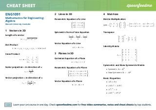
5 Determinants
2x2 Matrix
det
a b
c d
=
a b
c d
= ad − cb
3x3 Matrix
a b c
d e f
g h i
= a
e f
h i
− b
d f
g i
+ c
d e
g h
6 Inverse Matrices
2x2 Matrix
A−1
=
a b
c d
−1
=
1
ad − bc
d −b
−c a
Inverse Using Gaussian Elimination
Step 1 Augment with identity matrix [A|I]
Step 2 Row reduce to get [I|A−
1]
Inverse Using Determinants
Step 1 Select a row I and column J of matrix A
Step 2 Compute (−1)i+j (SJI)
det(A)
Step 3 Store at row J column I in inverse matrix
Step 4 Repeat for all entries
7 Eigenvalues and Eigenvectors
Av = λv
A is a square matrix, v is the eigenvector (a vector), λ is
the eigenvalue (a scalar).
Characteristic Equation
0 = det(A − λI) =
a1,1 − λ a1,2 · · · a1,n
a2,1 a2,2 − λ · · · a2,n
a3,1 a3,2 · · · a3,n
...
...
...
...
an,1 an,2 · · · an,n − λ
Eigendecomposition
Given matrix A with eigenvectors u, v, w and eigenvalues
α,β,γ:
A =
u1 v1 w1
u2 v2 w2
u3 v3 w3
α 0 0
0 β 0
0 0γ
u1 u2 u3
v1 v2 v3
w1 w2 w3
Powers/Inverses Using Eigendecomposition
An
=
u1 v1 w1
u2 v2 w2
u3 v3 w3
αn
0 0
0 βn
0
0 0γn
u1 u2 u3
v1 v2 v3
w1 w2 w3
8 Hyperbolic Functions
sinh x =
eu
− e−u
2
cosh x =
eu
+ e−u
2
Properties of Hyperbolic Functions
cosh2
x − sinh2
x = 1
d
dx
(cosh x) = sinh x
d
dx
(sinh x) = cosh x
cosh(u + v) = cosh u cosh v + sinh u sinh v
sinh(u − v) = sinh u cosh v − sinh v cosh u
2 cosh2
x = 1 + cosh 2x
2 sinh2
x = −1 + cosh 2x
9 Integration
Basic Integrals to Remember
ex
dx = ex
+ C
cos xdx = sin x + C
sin xdx = − cos x + C
xn
dx =
xn+1
n + 1
+ C (n = −1)
1
x
dx = loge(x) + C
9.1 Integration By Substitution
I = f(x) dx = f(x(u))
dx
du
du
2](data:image/gif;base64,R0lGODlhAQABAIAAAAAAAP///yH5BAEAAAAALAAAAAABAAEAAAIBRAA7)
Recommended
More Related Content
Recently uploaded
Recently uploaded (20)
Featured
Featured (20)
ENG1091 Past Paper Summary | Monash University
- 1. Learnyourunicourseinoneday.Checkspoonfeedme.com forfreevideosummaries,notesandcheatsheetsbytopstudents. CHEATSHEET ENG1091 Mathematics for Engineering: Algebra Monash University, Australia 1 Vectors in 3D Length of a vector |v| = x2 + y2 + z2 Dot Product v · w = vxwx + vywy + vzwz = |v||w|cosθ Cross Product v × w = ˆi ˆj ˆk vx vy vz wx wy wz Scalar projection v in direction of w vw = v · w |w| Vector projection v in direction of w vw = v · w |w|2 w 2 Lines in 3D Parametric Equation of a Line x(t) = a + pt y(t) = b + qt z(t) = c + rt Symmetric Form of Line Equation x − a p = y − b q = z − c r Vector Equation of a Line r(t) = d + tv 3 Planes in 3D Cartesian Equation of a Plane ax + by + cz = d Parametric Equation of a Plane x(u, v) = a + pu + lv y(u, v) = b + qu + mv z(u, v) = c + ru + nv Vector Equation of a Plane n · (r − d) = 0 4 Matrices Matrix Multiplication AB = a b c x y z α ρ β σ γ τ = aα + bβ + cγ aρ + bσ + cτ xα + yβ + zγ xρ + yσ + zτ Transpose a b c d e f T = a c e b d f Identity Matrix In = 1 0 0 · · · 0 0 1 0 · · · 0 0 0 1 · · · 0 ... ... ... ... ... 0 0 0 · · · 1 Symmetric and Skew Symmetric Matrix • Symmetric: A = AT • Skew-Symmetric: A = −AT Basic Properties • AB = BA • (AB)C = A(BC) • (AT )T = A • (AB)T = BT AT 1
- 2. Learnyourunicourseinoneday.Checkspoonfeedme.com forfreevideosummaries,notesandcheatsheetsbytopstudents. CHEATSHEET 5 Determinants 2x2 Matrix det a b c d = a b c d = ad − cb 3x3 Matrix a b c d e f g h i = a e f h i − b d f g i + c d e g h 6 Inverse Matrices 2x2 Matrix A−1 = a b c d −1 = 1 ad − bc d −b −c a Inverse Using Gaussian Elimination Step 1 Augment with identity matrix [A|I] Step 2 Row reduce to get [I|A− 1] Inverse Using Determinants Step 1 Select a row I and column J of matrix A Step 2 Compute (−1)i+j (SJI) det(A) Step 3 Store at row J column I in inverse matrix Step 4 Repeat for all entries 7 Eigenvalues and Eigenvectors Av = λv A is a square matrix, v is the eigenvector (a vector), λ is the eigenvalue (a scalar). Characteristic Equation 0 = det(A − λI) = a1,1 − λ a1,2 · · · a1,n a2,1 a2,2 − λ · · · a2,n a3,1 a3,2 · · · a3,n ... ... ... ... an,1 an,2 · · · an,n − λ Eigendecomposition Given matrix A with eigenvectors u, v, w and eigenvalues α,β,γ: A = u1 v1 w1 u2 v2 w2 u3 v3 w3 α 0 0 0 β 0 0 0γ u1 u2 u3 v1 v2 v3 w1 w2 w3 Powers/Inverses Using Eigendecomposition An = u1 v1 w1 u2 v2 w2 u3 v3 w3 αn 0 0 0 βn 0 0 0γn u1 u2 u3 v1 v2 v3 w1 w2 w3 8 Hyperbolic Functions sinh x = eu − e−u 2 cosh x = eu + e−u 2 Properties of Hyperbolic Functions cosh2 x − sinh2 x = 1 d dx (cosh x) = sinh x d dx (sinh x) = cosh x cosh(u + v) = cosh u cosh v + sinh u sinh v sinh(u − v) = sinh u cosh v − sinh v cosh u 2 cosh2 x = 1 + cosh 2x 2 sinh2 x = −1 + cosh 2x 9 Integration Basic Integrals to Remember ex dx = ex + C cos xdx = sin x + C sin xdx = − cos x + C xn dx = xn+1 n + 1 + C (n = −1) 1 x dx = loge(x) + C 9.1 Integration By Substitution I = f(x) dx = f(x(u)) dx du du 2
- 3. Learnyourunicourseinoneday.Checkspoonfeedme.com forfreevideosummaries,notesandcheatsheetsbytopstudents. CHEATSHEET Integration By Parts u dv = uv − v du Improper Integrals Examples: ∞ 0 x dx or 1 0 1 x dx or 1 −1 1 x dx Strategy: lim →∞ 0 x dx or lim →0 1 1 x dx 10 Series and Sequences Arithmetic an = an−1 + d = a + nd Sn = (n + 1)a + n(n + 1)d 2 Fibonacci Fn = Fn − 1 + Fn − 2 Geometric an = san−1 = a0sn Partial sums for geometric series Sn = (n + 1)a0 : s = 1 (1 − sn+1 )a0 1 − s : s = 1 Power Series In x around the point x = a: a0 + a1(x − a) + a2(x − a)2 + ... + an(x − a)n + ... = Σ∞ n=0an(x − a)n Maclaurin Series f(x) = a0 + a1x + a2x2 + ... + anxn + ... with: an = 1 n! dn f dxn x=0 Taylor Series If f(x) is infinitely differentiable at x=0, then: f(x) = a0 + a1(x − 1) + a2(x − a)2 + ... + an(x − a)n + ... with: an = 1 n! dn f dxn x=a 11 Convergence Tests For Improper Integrals Given I = ∞ 0 f(x) dx f(x) > 0 Convergence Find c(x) such that 1. 0 < f(x) < c(x) 2. lim →∞ 0 c(x) dx is finite Divergence Find d(x) such that 1. 0 < d(x) < f(x) 2. lim →∞ 0 c(x) dx = ∞ Comparison Test If C = Σ∞ n=0cn is a convergent series and D = Σ∞ n=0dn a divergent one then: Convergence: When 0 < an < cn ∀n > m Divergence: When 0 < dn < an ∀n > m Integral Test Given S = Σ∞ k=0ak with ak = f(k) take: lim n→∞ < ∞ 0 f(x) dx < lim n to∞ Sn−1 Convergence: Improper integral converges Divergence: Improper integral diverges Ratio Test Take: L = lim n→∞ an+1 an Then: Convergence: L < 1 Divergence: L > 1 Indeterminate: L = 1 3
- 4. Learnyourunicourseinoneday.Checkspoonfeedme.com forfreevideosummaries,notesandcheatsheetsbytopstudents. CHEATSHEET Alternating Series If |an| → ∞: Convergence: When |an+1| < |an| ∀n > m Divergence: Otherwise Absolute Convergence If Σ∞ n=0|an| converges then Σ∞ n=0an converges absolutely, otherwise we can’t say anything. 12 Taylor Series Useful Functions ex = 1 + x + x2 2! + x3 3! + ... = Σ∞ n=0 xn n! cos x = 1 − x2 2! + x4 4! − x6 6! + ... = Σ∞ n=0(−1)n x2n 2n! sin x = x − x3 3! + x5 5! − x7 7! + ... = Σ∞ n=0(−1)n+1 x2n+1 (2n + 1)! Error Bound En = |f(x) − Pn(x)| < M (n + 1) Rn+1 M is the maximum value of |f(n+1) (x)| in |x − a| < R With Remainder Term f(x) = Pn(x) + En(x) With: Pn(x) = f(a) + (x − a)f (a) + (x − a)2 2! f (a) + ... + (x − a)n n! f(n) (a) And En(x) = x a (−1)n (u − x)n n! f(n+1) (u) du 13 l’Hopital’s Rule lim x→a f(x) g(x) = lim x→a f (x) g (x) lim x→a f(x) = lim x→a g(x) = 0 or = ∞ 14 1st Linear Order ODEs Separable If dy dx = f(x) g(y) , set g(y) dy = f(x) dx Integrating Factor To solve: dy dx + P(x)y = Q(x) Use: y(x) = 1 I(x) I(x)Q(x) dx Where: I(x) = e P (x) dx 15 2nd Order Linear ODEs Linear, Homogeneous For: a d2 y dx2 + b dy dx + cy = 0 Characteristic Equation: aλ2 + bλ + c = 0 If λ1 and λ2 are the roots: Case 1: λ1 = λ2 and real ⇒ y(x) = Aeλ1x + Beλ2x Case 2: λ = α ± iβ ⇒ y(x) = eαx (A cos(βx) + B sin(βx)) Case 3: λ1 = λ2 ⇒ y(x) = (A + Bx)eλx 4
- 5. Learnyourunicourseinoneday.Checkspoonfeedme.com forfreevideosummaries,notesandcheatsheetsbytopstudents. CHEATSHEET Non-homogeneous Method of Undetermined Coefficients Given: a d2 y dx2 + b dy dx + cy = S(x) Guesses for various S(x): For: S(x) = (a + bx + cx2 + ... + dxn )ekx Try: yp(x) = (e + fx + gx2 + ... + hxn )ekx For: S(x) = (a sin(bx) + c cos(bx))ekx Try: yp(x) = (d cos(bx) + f sin(bx))ekx 16 Coupled Systems of ODEs Given the homogeneous equation ˙y = Ay: Step 1: Find eigenvalues of A Step 2: For each eigenvalue λ find the eigenvector v Step 3: For each pair (λ, v) a solution is given by the Euler’s Guess y = eλx v 17 Functions of Several Variables Chain Rule Along a path x = x(s), y = y(s): df ds = ∂f ∂x dx ds + ∂f ∂y dy ds If x = x(u, v) and y = y(u, v) then: ∂f ∂u = ∂f ∂x ∂x ∂u + ∂f ∂y ∂y ∂u ∂f ∂v = ∂f ∂x ∂x ∂v + ∂f ∂y ∂y ∂v Directional Derivative Of function f in direction of unit vector t: df ds = t · f = tf where: f = ∂f ∂x ˆi + ∂f ∂y ˆj Tangent Plane The tangent plane to f = f(x, y) at P is: ˜f(x, y) = fP + (x − a) ∂f ∂x P + (y − b) ∂f ∂y P Finding and Classifying Extrema Extrema at: f = 0 Let: D = ∂2 f ∂x2 ∂2 f ∂y2 − ∂2 f ∂x∂y 2 Then: Local Minima: D ≥ 0 and ∂2 f ∂x2 > 0 Local Maxima: D ≥ 0 and ∂2 f ∂x2 < 0 Saddle Point: D < 0 5