ENGINEERING MATERIALS AND METALLURGY.pptx

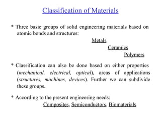
Classification of Materials
* Three basic groups of solid engineering materials based on
atomic bonds and structures:
Metals
Ceramics
Polymers
* Classification can also be done based on either properties
(mechanical, electrical, optical), areas of applications
(structures, machines, devices). Further we can subdivide
these groups.
* According to the present engineering needs:
Composites, Semiconductors, Biomaterials

Metals
* Characteristics are owed to non-localized electrons (metallic
bond between atoms) i.e. electrons are not bound to a
particular atom.
They are characterized by their high thermal and electrical
conductivities.
They are opaque, can be polished to high lustre. The opacity
and reflectivity of a metal arise from the response of the
*
*
unbound electrons to electromagnetic vibrations at light
frequencies.
Relatively heavier, strong, yet deformable.
*
E.g.: Steel, Aluminium, Brass, Bronze, Lead, Titanium, etc.

Ceramics
*
*
They contain both metallic and nonmetallic elements.
Characterized by their higher resistance to high temperatures
and harsh environments than metals and polymers.
Typically good insulators to passage of both heat and
electricity.
Less dense than most metals and alloys.
They are harder and stiffer, but brittle in nature.
They are mostly oxides, nitrides, and carbides of metals.
Wide range: traditional (clay, silicate glass, cement) to
advanced (carbides, pure oxides, non-silicate glasses).
*
*
*
*
*
E.g.: Glass, Porcelain, Minerals, etc.

Polymers
* Commercially called plastics; noted for their low density,
flexibility and use as insulators.
Mostly are of organic compounds i.e. based on carbon,
oxygen and other nonmetallic elements.
Consists large molecular structures bonded by covalent and
van der Waals forces.
They decompose at relatively moderate temperatures (100-
400 C).
Application: packaging, textiles, biomedical devices, optical
devices, household items, toys, etc.
*
*
*
*
E.g.: Nylon, Teflon, Rubber, Polyester, etc.

Composites
* Consist more than one kind of material; tailor made to benefit
from combination of best characteristics of each constituent.
Available over a very wide range: natural (wood) to synthetic
(fiberglass).
Many are composed of two phases; one is matrix – which is
continuous and surrounds the other, dispersed phase.
Classified into many groups: (1) depending on orientation of
phases; such as particle reinforced, fiber reinforced, etc. (2)
depending on matrix; metal matrix, polymer matrix, ceramic
matrix.
*
*
*
E.g.: Cement concrete, Fiberglass, special purpose refractory
bricks, plywood, etc.

Semiconductors
* Their electrical properties are intermediate when compared
with electrical conductors and electrical insulators.
* These electrical characteristics are extremely sensitive to the
presence of minute amounts of foreign atoms.
* Found very many applications in electronic devices over
decades through integrated circuits. In can be said that
semiconductors revolutionized the electronic industry for last
few decades.

Biomaterials
* Those used for replacement of damaged or diseased body
parts.
Primary requirements: must be biocompatible with body
tissues, must not produce toxic substances.
Important materials factors: ability to support the forces, low
friction and wear, density, reproducibility and cost.
All the above materials can be used depending on the
application.
A classic example: hip joint.
*
*
*
*
E.g.: Stainless steel, Co-28Cr-6Mo, Ti-6Al-4V, ultra high
molecular weight polyethelene, high purity dense Al-oxide,
etc.

Advanced materials
* Can be defined as materials used in high-tech devices i.e.
which operates based on relatively intricate and sophisticated
principles (e.g. computers, air/space-crafts, electronic
gadgets, etc.).
These are either traditional
* materials with enhanced
properties or newly developed materials with high-
performance
expensive.
capabilities. Thus, these are relatively
* Typical applications: integrated circuits, lasers, LCDs, fiber
optics, thermal protection for space shuttle, etc.
E.g.: Metallic foams, inter-metallic compounds, multi-
component alloys, magnetic alloys, special ceramics and high
temperature materials, etc.

Future materials
* Group of new and state-of-the-art materials now being
developed, and expected to have significant influence on
present-day technologies, especially
manufacturing and defense.
Smart/Intelligent material system
in the fields of medicine,
* consists some type of
sensor (detects an input) and an actuator (performs
responsive and adaptive function).
Actuators may be called upon to
* change shape, position,
natural frequency, mechanical characteristics in response to
changes
pH, etc.
in temperature, electric/magnetic fields, moisture,

Future materials (contd…)
* Four types of materials used as actuators:
-
-
-
-
Shape memory alloys
Piezoelectric ceramics
Magnetostrictive materials
Electro-/Magneto-rheological fluids
* Materials / Devices used as sensors:
-
-
-
-
Optical fibers
Piezoelectric materials
Micro-electro-mechanical systems (MEMS)
etc.

Future materials (contd…)
* Typical applications:
- By incorporating sensors, actuators and chip processors into
system, researchers are able to stimulate biological human-
like behavior.
- Fibers for bridges, buildings, and wood utility poles.
- They also help in fast moving and accurate robot parts, high
speed helicopter rotor blades.
- Actuators that control chatter in precision machine tools.
- Small microelectronic circuits in machines ranging from
computers to photolithography prints.
- Health monitoring detecting the success or failure of a
product.

Modern materials’ needs
* Engine efficiency increases at high temperatures; requires
high temperature structural materials.
* Use of nuclear energy requires solving problems with
residue, or advance in nuclear waste processing.
* Hypersonic flight requires materials that are light, strong and
resist high temperatures.
* Optical communications require optical fibers that absorb
light negligibly.
* Civil construction – materials for unbreakable windows.
* Structures: materials that are strong like metals and resist
corrosion like plastics.

Material Science
Module-2
Structures,
Atomic Interatomic
Bonding and Structure of
Crystalline Solids

Contents
Atomic Structure and Atomic
solids
Crystal structures, Crystalline
crystalline materials
1) bonding in
2) and Non-
3) Miller indices, Anisotropic elasticity
Elastic behavior of Composites
Structure and properties of polymers
Structure and properties of ceramics
and
4)
5)

Atomic structure
* Every atom consists of a small nucleus composed of
protons and neutrons, which is encircled by moving
electrons in their orbitals, specific energy levels.
In an atom, there will be always equal number of protons
and electrons
The top most orbital electrons, valence electrons, affect
*
*
most material properties that are of interest to engineer.
E.g.: chemical properties, nature of bonding, size of atom,
optical/magnetic/electrical properties.
Electrons and protons are negative and positive charges of
the same magnitude being 1.60x10-19 coulombs.
Neutrons are electrically neutral.
Protons and neutrons have approximately the mass,
1.67x10-27 kg, which is larger than that of an electron,
9.11x10-31 kg.
*
*
*

Atomic structure (contd…)
*
*
Atomic number (Z) - is the number of protons per atoms.
Atomic mass (A) - is the sum of the masses of protons and
neutrons within the nucleus.
Atomic mass is measured in atomic mass unit (amu) where
1amu=(112) the mass of most common isotope of carbon
atom, measured in grams.
A ≅ Z+N, where N is number of neutrons.
Isotopes - atoms with same atomic number but different
atomic masses.
A mole is the amount of matter that has a mass in grams
equal to the atomic mass in amu of the atoms. Thus a mole
of carbon has a mass of 12 grams.
*
*
*
*

Atomic structure (contd…)
* The number of atoms or molecules in a mole of substance is
called the Avogadro’s number, Nay. Nay=1gram/1amu =
6.023x1023.
E.g.: Calculating the number of atoms per cm3, n, in a piece of
material of density δ (g/cm3)
× δ / M,
n = Nav where M is the atomic mass in amu.
Thus, for graphite (carbon) with a density δ = 1.8 g/cm3 and M =12, n =
1023 atoms/mol × 1.8 g/cm3 / 12 g/mol) = 9 × 1022 atoms/cm3.
6.023 ×
* Most solid materials will have atomic density in the order of
6x1022, that’s about 39 million atoms per centimeter.
Mean distance between atoms is in the range of 0.25 nm. It
*
gives an idea about scale of atomic structures in solids.

Atomic Bonding in Solids
* Two questions need to be answered: why the atoms are
clustered together?, and how they are arranged?
* Bonds are two kinds – Primary, and Secondary
* Primary bonds – relatively stronger. Exists in almost all solid
materials.
E.g.: Ionic, Covalent, and Metallic bonds.
* Secondary bonds – relatively weaker bonds. Exists in many
substances like water along with primary bonds.
E.g.: Hydrogen, and van der Waals forces.

Atomic Bond in Solids
permanent
Polar
induced
Fluctuating
induced
covalent
ionic metallic
Secondary bonding
Primary bonding
Atomic bonding

Primary inter-atomic bonds
* These bonds invariably involves valence electrons.
* Nature of bond depends on electron arrangement in respective
atoms.
* Atoms tend to acquire stable electron arrangement in their
valence orbitals by transferring (ionic), sharing (covalent, and
metallic) valence electrons. This leads to formation of bonds.
* Bond energies are in order of 1000 kJ/mol.

Ionic bond
* This primary bond exists between two atoms when transfer of
electron(s) results in one of the atoms to become negative (has
an extra electron) and another positive (has lost an electron).
This bond is a direct consequence of strong Coulomb
attraction between charged atoms.
Basically ionic bonds are non-directional in nature.
In real solids, ionic bonding is usually exists along with
covalent bonding.
*
*
*
E.g.: NaCl. In the molecule, there are more electrons around
Cl, forming Cl- and fewer electrons around Na, forming Na+.

Na+ Cl-
Fig.1 Schematic representation of ioning bonding.
Here, Na is giving an electron to Cl to have stable structure

Covalent bond
* This bond comes into existence if valence electrons are shared
between a pair of atoms, thus acquire stability by saturating
the valence configuration.
Covalent bonds are stereospecific i.e. each bond is between a
specific pair of atoms, which share a pair of electrons (of
opposite magnetic spins).
Typically, covalent bonds are very strong, and directional in
nature.
*
*
E.g.: H2 molecule, where an electron from each of the atom
shared by the other atom, thus producing the covalent bond.

H H
Figure 2. Schematic representation of covalent bond in
Hydrogen molecule (sharing of electrons)

Metallic bond
* This bond comes into existence if valence electrons are shared
between number of atoms, i.e. arranged positive nucleuses are
surrounded by electron pool.
Shared electrons are not specific to a pair of atoms, in contrast
to Covalent bond, i.e. electrons are delocalized.
As shared electrons are delocalized, metallic bonds are non-
directional.
Very characteristic properties of metals like high thermal and
electrical conductivities are result of presence of delocalized
electron pool.
*
*
*

Electron cloud from the valence electrons
M M M M
Core
M M M M
M M M M
M M M M
Figure 3. Metallic bonding

Secondary inter-atomic bonds
* These bonds involves atomic or molecular dipoles.
* Bonds can exists between induced and permanent dipoles
(polar molecules).
* Bond comes into existence because of Columbic attraction
between positive end of one dipole and negative end of
another dipole.
* Bond energies are in order of 10 kJ/mol

Figure 4. Dipole bonds in water

Secondary inter-atomic bonds (contd...)
* Existence of these depends on three kinds of dipoles –
fluctuating dipoles, Polar-molecule dipoles and Permanent
dipoles.
* Permanent dipole bonds are also called Hydrogen bonds as
covalently bonded hydrogen atoms – for example C-H, O-H,
F-H – share single electron becomes positively charged
proton that is capable of strong attractive force with the
negative end of an adjacent molecule.
* Hydrogen bonds is responsible for water to exist in liquid
state at room temperature.

Crystal Structures
* All solid materials are made of atoms/molecules, which are
arranged in specific order in some materials, called crystalline
solids. Otherwise non-crystalline or amorphous solids.
* Groups of atoms/molecules specifically arranged – crystal.
* Lattice is used to represent a three-dimensional periodic array
of points coinciding with atom positions.
* Unit cell is smallest repeatable entity that can be used to
completely represent a crystal structure. It is the building
block of crystal structure.

Unit cell
It is characterized by:
*
*
*
*
Type of atom and their radii, R
Cell dimensions (Lattice spacing a, b and c) in terms of R and
Angle between the axis α, β, γ
a*, b*, c* - lattice distances in reciprocal lattice , α*, β*, γ* -
angles in reciprocal lattice
Number of atoms per unit cell, n
Coordination number (CN)– closest neighbors to an atom
Atomic packing factor, APF
Most common unit cells – Face-centered cubic, Body-
centered cubic and Hexagonal.
*
*
*

Common Crystal Structures
Unit Cell n CN a/R APF
Simple Cubic 1 6 4/√ 4 0.52
Body-Centered Cubic 2 8 4/√ 3 0.68
Face-Centered Cubic 4 12 4/√ 2 0.74
Hexagonal Close Packed 6 12 0.74

Miller indices
* A system of notation is required to identify particular
direction(s) or plane(s) to characterize the arrangement of
atoms in a unit cell
Formulas involving Miller indices are very similar to related
formulas from analytical geometry – simple to use
Use of reciprocals avoids the complication of infinite
intercepts
Specifying dimensions in unit cell terms means that the same
label can be applied to any plane with a similar stacking
pattern, regardless of the crystal class of the crystal. Plane
(111) always steps the same way regardless of crystal system
*
*
*

Miller indices - Direction
* A vector of convenient length is placed parallel to the
required direction
* The length of the vector projection on each of three axes are
measured in terms of unit cell dimensions
* These three numbers are made to smallest integer values,
known as indices, by multiplying or dividing by a common
factor
* The three indices are enclosed in square brackets, [uvw].
* A family of directions is represented by <uvw>

Miller indices - Plane
* Determine the intercepts of the plane along the
crystallographic axes, in terms of unit cell dimensions. If
plane is passing through origin, there is a need to construct
plane parallel to original plane
* Take the reciprocals of these intercept numbers
* Clear fractions
* Reduce to set of smallest integers
* The three indices are enclosed in parenthesis, (hkl).
* A family of planes is represented by {hkl}
a

Miller indices – Useful Conventions
* If a plane is parallel to an axis, its intercept is at infinity and
its Miller index will be zero
Never alter negative numbers. This implies symmetry that the
crystal may not have! Use bar over the number to represent
negative numbers.
A plane or direction of family is not necessarily parallel to
other planes or directions in the same family
The smaller the Miller index, more nearly parallel the plane
to that axis, and vice versa
Multiplying or dividing a Miller index by constant has no
effect on the orientation of the plane
When the integers used in the Miller indices contain more
than one digit, the indices must be separated by commas. E.g.:
(3,10,13)
*
*
*
*
*

Useful Conventions for cubic crystals
* [uvw] is normal to (hkl) if u = h, v = k, and w = l. E.g.: (111)
┴ [111]
[uvw] is parallel to (hkl) if hu + kv + lw = 0
Two planes (h1k1l1) and (h2k2l2) are normal if h1h2 + k1k2
+ l1l2=0
Two directions (u1v1w1) and (u2v2w2) are normal if u1u2 +
v1v2 + w1w2=0
Inter-planar distance between family of planes {hkl} is given
*
*
*
*
by: a
=
d {hkl }
2 2 2
h + k + l
* Angle between two planes is given by:
h1h2 +k1k2 +l1l2
cosθ
= h2
k 2
l 2
h2
k 2
l 2
+ + + +
1 1 1 2 2 2

Miller-Bravis indices
* Miller indices can describe all possible planes/directions in
any crystal.
However, Miller-Bravis indices are used in hexagonal
systems as they can reveal hexagonal symmetry more clearly
Indices are based on four axes – three are coplanar on basal
*
*
plane at 120˚ apart, fourth axis is perpendicular to basal
Both for planes/directions, extra index is given by
t = -(u+v), i = -(h+k)
where plane is represented as [uvtw], and a direction is
represented by (hkil)
plane
*
E.g.: Basal plane – (0001), Prismatic plane – (10ֿ10)

Polymers - definition
*
*
Polymers are made of basic units called mers
These are usually Hydrocarbons – where major constituent
atoms are Hydrogen and Carbon
When structure consists of only one mer, it is monomer. If it
contains more than one mer, it is called polymer
Isomers are molecules those contain same number of similar
mers but arrangement will be different
E.g.: Butene and Isobutene
When a polumer has ONE kind of mers in its structure, it is
called homopolymer
Polymer made with more than one kind of mers is called
copolymer
*
*
*
*

Polymer structures
* Linear, where mer units are joined together end to end in
single chains. E.g.: PVC, nylon.
Branched, where side-branch chains are connected to main
ones. Branching of polymers lowers polymer density because
of lower packing efficiency E.g.: Bakelite
Cross-linked, where chains are joined one to another at
various positions by covalent bonds. This cross-linking is
usually achieved at elevated temperatures by additive atoms.
E.g.: vulcanization of rubber
Network, trifunctional mer units with 3-D networks comes
under this category. E.g.: epoxies, phenol-formaldehyde.
*
*
*

Polymer structures
Schematic presentation of polymer structures.
Individual mers are represented by solid circles.

Thermo-sets – Thermo-plasts
* Polymers mechanical response at elevated temperatures
strongly depends on their chain configuration
Based on this response polymers are grouped in to two -
thermo-sets and thermo-plasts
Thermo-sets: become permanently hard when heated, and do
not soften during next heat cycle. During first heating
covalent bonds forms thus extensive cross-linking takes place.
Stronger and harder than thermo-plasts.
E.g.: Vulcanized rubber, epoxies, some polyester resins
Thermo-plasts: softens at high temperatures, and becomes
hard at ambient temperatures. The process is reversible.
Usually made of linear and branched structures.
E.g.: Polystyrene, Acrylics, Cellulosics, Vinyls
*
*
*

Polymer crystallinity
*
*
Crystallinity in polymers is more complex than in metals
Polymer crystallinity range from almost crystalline to
amorphous in nature
It depends on cooling path and on chain configuration
Crystalline polymers are more denser than amorphous
polymers
Many semicrystalline polymers form spherulites. Each
spherulite consists of collection of ribbon like chain folded
lamellar crystallites.
*
*
*
E.g.: PVC (Poly Vinyl Chloride)

Ceramics
* Ceramics are inorganic and non-metallic materials
* Atomic bonds in ceramics are mixed – covalent + ionic
* Proportion of bonds is specific for a ceramic
* Ionic bonds exists between alkalis/alkaline-earth metals and
oxygen/halogens.
* Mostly oxides, carbides, nitrides of metals are ceramics
E.g.: Sand, Glass, Bricks, Marbles

Ceramic structures
* Building criteria for ceramic structures:
- maintain neutrality
- closest packing
* Packing efficiency can be characterized by coordination
number which depends on cation-anion radius ratio (rc/ra)
1.000
Cation-anion
radius ratio
(rc/ra)
<
0.155
0.155 –
0.225
0.225 –
0.414
0.414 –
0.732
0.732 –
1.000
>
Coordination
number
2 3 4 6 8 12

Ion arrangement – Coordination numbers

Ceramic crystal structures
* AX-type: most common in ceramics. They assume different
structures of varying coordination number (CN).
Rock salt structure – CN=6.
Cesium Chloride structure – CN=8
Zinc Blende structure – CN=4
E.g.:
E.g.:
E.g.:
NaCl, FeO
CsCl
ZnS, SiC
* AmXp-type: number of anions and cations are different (m≠p).
One unit cell is made of eight cubes.
E.g.: CaF2, ThO2
* AmBnXp-type: when ceramic contains more then one kind of
cations. Also called perovskite crystal structure.
E.g.: BaTiO3

Silicates
* Most common ceramic in nature – Silicates, as constituent
elements – silicon and oxygen – are most abundant in earth’s
crust.
Si4+ O2-
* Bond between and is weak ionic and very strong
covalent in nature. Thus, basic unit of silicates is SiO4
4-
tetrahedron.

Silicates (contd…)
* In Silica (SiO2), every oxygen atom the corner of the
tetrahedron is shared by the adjacent tetrahedron.
Silica can be both crystalline (quartz) and amorphous (glass)
Crystalline forms of silica are complicated, and comparatively
open…thus low in density compared with amorphous glasses
Addition of network modifiers (Na2O) and intermediates
(Al2O3, TiO2)lowers the melting point…thus it is easy to
form. E.g.: Bottles.
In complicated silicates, corner oxygen is shared by other
tetrahedra….thus consists SiO4
4-, Si2O7
6-, Si3O9
6- groups
Clays comprises 2-D sheet layered structures made of Si2O5
2-
*
*
*
*
*

Carbon
* Carbon is not a ceramic, but its allotropic form - Diamond - is
* Diamond:
C-C covalent bonds, highest known hardness,
Semiconductor, high thermal conductivity, meta-stable
* Graphite - another allotropic form of carbon
layered structure - hexagonal bonding within planar
leyers, good electrical conductor, solid lubricant
* Another allotropic form - C60 - also called Fullerene / Bucky
ball. Structure resembles hallow ball made of 20 hexagons
and 12 pentagons where no two pentagons share a common
edge.
* Fullerenes and related nanotubes are very strong, ductile -
could be one of the important future engineering materials

Imperfections in ceramics
* Imperfections in ceramics – point defects, and impurities.
Their formation is strongly affected by charge neutrality
* Frenkel-defect is a vacancy-interstitial pair of cations
* Schottky-defect is a pair of nearby cation and anion vacancies
* Impurities:
Introduction of impurity atoms in the lattice is likely in
conditions where the charge is maintained.
E.g.: electronegative impurities that substitute lattice
anions or electropositive substitutional impurities

Mechanical response of ceramics
* Engineering applications of ceramics are limited because of
presence of microscopic flaws – generated during cooling
stage of processing.
However, as ceramics are high with hardness, ceramics are
good structural materials under compressive loads.
Plastic deformation of crystalline ceramics is limited by
strong inter-atomic forces. Little plastic strain is accomplished
by process of slip.
Non-crystalline ceramics deform by viscous flow.
Characteristic parameter of viscous flow – viscosity.
Viscosity decreases with increasing temperature. However, at
room temperature, viscosity of non-crystalline ceramics is
very high.
*
*
*
*

Mechanical response of ceramics (contd…)
* Hardness – one best mechanical property of ceramics which
is utilized in many application such as abrasives, grinding
media
Hardest materials known are ceramics
Ceramics having Knoop hardness about 1000 or greater are
used for their abrasive characteristics
Creep – Ceramics experience creep deformation as a result of
exposure to stresses at elevated temperatures.
Modulus of elasticity, E, as a function of volume fraction of
porosity, P: E = E0 (1-1.9 P + 0.9 P2)
Porosity is deleterious to the flexural strength for two reasons:
- reduces the cross-sectional area across where load is applied
- act as stress concentrations
*
*
*
*
*

Material Science
Module-3
Imperfections in Solids

Contents
1) Theoretical yield strength, Point defects
and Line defects or Dislocations
2) Interfacial defects, Bulk or Volume defects
and Atomic vibrations

Theoretical yield strength
* Ideal solids are made of atoms arranged in orderly way.

Theoretical yield strength (contd…)
* Using a sin function to represent the variation in shear
stress
Gx
2Πx
b
2Πx
b
τ = Gγ =
τ ≈ τ
τ =τ sin m
a
m
(Hooke’s law)
G b
τ =
m
2Π a
If b≈a
τ
G
=
m
2Π
G ≈ 20-150 GPa
Shear strength ≈ 3-30 GPa
(ideal)
Real strength values ≈ 0.5-10 MPa

Theoretical yield strength (contd…)
* Theoretical strength of solids shall possess an ideal value
in the range of 3-30 GPa.
* Real values observed in practice are 0.5-10 MPa.
* The assumption of perfectly arranged atoms in a solid may
not valid…..i.e. atomic order must have been disturbed.
* Disordered atomic region is called defect or imperfection.
* Based on geometry, defects are: Point defects (zero-D),
Line defects (1-D) or Dislocations, Interfacial defects (2-
D) and Bulk or Volume defects (3-D).

Point defects
* Point defects are of zero-dimensional i.e. atomic disorder
is restricted to point-like regions.
* Thermodynamically stable compared with other kind of
defects.

Point defects (contd…)
* Fraction of vacancy sites can be given as follows:
n −Q
= e kT
N
* In ionic crystals, defects can form on the condition of
charge neutrality. Two possibilities are:

Line defects
* Line defects or Dislocations are abrupt change in atomic
order along a line.
* They occur if an incomplete plane inserted between perfect
planes of atoms or when vacancies are aligned in a line.
* A dislocation is the defect responsible for the phenomenon
of slip, by which most metals deform plastically.
Dislocations occur in high densities (108-1010 m-2
* ), and are
intimately connected to almost all mechanical properties
which are in fact structure-sensitive.
* Dislocation form during plastic deformation, solidification
or due to thermal stresses arising from rapid cooling.

Line defects – Burger’s vector
* A dislocation in characterized by Burger’s vector, b.
* It is unique to a dislocation, and usually have the
of close packed lattice direction. It is also the slip
of a dislocation.
direction
direction
* It represents the magnitude and direction of distortion
associated with that particular dislocation.
* Two limiting cases of dislocations, edge and screw, are
characterized by Burger’s vector perpendicular to the
the
of
dislocation
dislocation
line
line
(t) and Burger’s vector parallel to
is
respectively. Ordinary dislocation
mixed character of edge and screw type.

Line defects – Edge dislocation
* It is also called as Taylor-Orowan dislocation.
* It will have regions of compressive and tensile stresses on
either side of the plane containing dislocation.

Line defects – Screw dislocation
* It is also called as Burger’s dislocation.
* It will have regions of shear stress around the dislocation
line
* For positive screw dislocation, dislocation line direction is
parallel to Burger’s vector, and vice versa.
A negative
dislocation

Line defects – Dislocation motion
* Dislocations move under applied stresses, and thus causes
plastic deformation in solids.
Dislocations can move in three ways – glide/slip, cross-slip
*
and climb – depending on their character. Slip is
conservative in nature, while the climb is non-
conservative, and is diffusion-controlled.
Any dislocation can slip, but in the direction of its
vector.
Edge dislocation moves by slip and climb.
* burger’s
*
* Screw dislocation moves by slip / cross-slip. Possibility for
cross-slip arises as screw dislocation does not have a
preferred slip plane as edge dislocation have.

Line defects – Dislocation characteristics
* A dislocation line cannot end at abruptly inside a crystal. It
can close-on itself as a loop, either end at a node or
surface.
Burger’s vector for a dislocation line is invariant i.e. it
*
will have same magnitude and direction all along the
dislocation line.
Energy associated with a dislocation because of presence
*
of stresses is proportional to square of Burger’s vector
length. Thus dislocations, at least of same nature, tend to
stay away from each other.
Dislocations are, thus, two types – full and partial
*
dislocations. For full dislocation, Burger’s vector is
integral multiple of inter-atomic distance while for partial
dislocation, it is fraction of lattice translation.

Interfacial defects
* An interfacial defect is a 2-D imperfection in crystalline
solids, and have different crystallographic orientations on
either side of it.
* Region of distortion is about few atomic distances.
* They usually arise from clustering of line defects into a
plane.
* These imperfections are not thermodynamically stable, but
meta-stable in nature.
E.g.: External surface, Grain boundaries, Stacking faults,
Twin boundaries, Dislocations and Phase boundaries.

Interfacial defects (contd…)
Grain boundaries

Bulk or Volume defects
* Volume defects are three-dimensional in nature.
* These defects are introduced, usually, during processing
and fabrication operations like casting, forming etc.
E.g.: Pores, Cracks, Foreign particles
* These defects act like stress raisers,
mechanical properties of parent solids.
thus deleterious to
* In some instances, foreign particles are added to strengthen
the solid – dispersion hardening. Particles added are
hindrances to movement of dislocations which have to cut
through or bypass the particles thus increasing the strength.

Atomic vibrations
* Atoms are orderly arranged, but they are expected to
vibrate about their positions where the amplitude of
vibration increases with the temperature.
* After reaching certain temperature, vibrations are vigorous
enough to rupture the inter-atomic forces casing melting
solids.
of
* Average amplitude of vibration at room temperature is
10-12m
about i.e. thousandth of a nanometer.
1013
* Frequency of vibrations is the range of Hz.
* Temperature of a solid body is actually a measure
vibrational activity of atoms and/or molecules.
of

Module-4
Mechanical Properties of Metals

Contents
1)
2)
3)
Elastic deformation and Plastic deformation
Interpretation of tensile stress-strain curves
Yielding under multi-axial stress, Yield
criteria, Macroscopic aspects of plastic
deformation and Property variability &
Design considerations

Mechanical loads - Deformation
Object
translation rotation deformation
distortion – change
dilatation – change
in shape
in size
External load

Deformation – function of time?
Temporary / recoverable Permanent
time independent –
plastic
time dependent –
creep (under load),
time independent –
elastic
time dependent –
anelastic (under load),
elastic aftereffect (after removal of load)
combination of recoverable and permanent, but time
dependent – visco-elastic

Engineering Stress – Engineering Strain
*
*
Load applied acts over an area.
Parameter that characterizes the load effect is given as load
divided by original area over which the load acts. It is
called conventional stress or engineering stress or simply
stress. It is denoted by s.
Corresponding change in length of the object is
characterized using parameter – given as per cent change
*
in the length – known as strain. It is denoted
L −L0
by e.
P
, e
s = =
A0 L0
* As object changes its dimensions under applied load,
true
engineering stress and strain are not be the
representatives.

True Stress – True Strain
* True or Natural stress and strain are defined to give true
picture of the instantaneous conditions.
* True strain:
L1 −L0 L2 −L1 L3 −L2
L
∫
L
dL
L
ln
L
∑
ε = + + +... ε = =
L0 L1 L2 L0
0
* True stress:
A0
P
A
P
σ = = = s(e +1)
A0 A

Elastic deformation
* A material under goes elastic deformation first followed by
plastic deformation. The transition is not sharp in many
instances.
* For most of the engineering materials, complete elastic
deformation is characterized by strain proportional to
or
stress. Proportionality constant
Young’s modulus, E.
σ ∝ ε
is called elastic modulus
σ = Eε
* Non-linear stress-strain
E.g.: rubber.
relation is applicable for materials.

Elastic deformation (contd…)
* For materials without linear stress-strain portion, either
tangent or secant modulus is used in design calculations.
The tangent modulus is
taken as the slope of
stress-strain curve at
some specified level.
Secant module
represents the slope of
secant drawn from the
origin to some given
point of the σ-ε curve.

* Theoretical basis for elastic deformation – reversible
displacements of atoms from their equilibrium positions –
stretching of atomic bonds.
* Elastic moduli measures stiffness of material. It can also be
a measure of resistance to separation of adjacent atoms.
* Elastic modulus = fn (inter-atomic forces)
= fn (inter-atomic distance)
= fn (crystal structure, orientation)
=> For single crystal elastic moduli are not isotropic.
* For a polycrystalline material, it is considered as isotropic.
* Elastic moduli slightly changes with temperature
(decreases with increase in temperature).

* Linear strain is always accompanied by lateral strain, to
maintain volume constant.
The ratio of lateral to linear strain is called Poisson’s ratio
(ν).
Shear stresses and strains are related as τ = Gγ, where G is
shear modulus or elastic modulus in shear.
Bulk modulus or volumetric modulus of elasticity is
*
*
*
defined as ratio between mean stress to
K = σm/Δ
All moduli are related through Poisson’s
volumetric strain.
* ratio.
E
E σm
G = K = =
2(1+ν) 3(1− 2ν)
Δ

Plastic deformation
* Following the elastic deformation, material undergoes
plastic deformation.
Also characterized by relation between stress and strain at
constant strain rate and temperature.
Microscopically…it involves breaking atomic bonds,
moving atoms, then restoration of bonds.
Stress-Strain relation here is complex because of atomic
plane movement, dislocation movement, and the obstacles
they encounter.
Crystalline solids deform by processes – slip and twinning
in particular directions.
Amorphous solids deform by viscous flow mechanism
without any directionality.
*
*
*
*
*

Plastic deformation (contd…)
* Because of the complexity involved, theory of plasticity
neglects the following effects:
- Anelastic strain, which is time dependent recoverable
strain.
- Hysteresis behavior resulting from loading and un-
loading of material.
- Bauschinger effect – dependence of yield stress on
loading path and direction.
Equations relating stress and strain are called constitutive
equations.
A true stress-strain curve is called flow curve as it gives the
stress required to cause the material to flow plastically to
certain strain.
*
*

Plastic deformation (contd…)
* Because of the complexity involved, there have been many
stress-strain relations proposed.
σ fn(ε,ε&,T,
microstructure)
=
n
σ Kε
= Strain hardening exponent, n = 0.1-0.5
Kε&
m
K (ε
σ = Strain-rate sensitivity, m = 0.4-0.9
)n
σ +ε
= Strain from previous work – ε0
0
n
σ =σ + Kε Yield strength – σ0
o

Tensile stress-strain curve
A – Starting point
E’ – Corresponding to E on
F – Fracture point
E– Tensile strength
flow curve
I – Fracture strain

Tensile stress-strain curve (contd…)
A – Starting point
C – Elastic limit
G – 0.2% offset strain
B – Proportional limit
D – Yield limit
H – Yield strain

Tensile stress-strain curve (contd…)
* Apart from different strains and strength points, two other
important parameters can be deduced from the curve are –
resilience and toughness.
* Resilience (Ur) – ability to absorb energy under elastic
deformation
* Toughness (Ut) – ability to absorb energy under loading
involving plastic deformation. Represents
both strength and ductility.
combination of
2
s0 s0
1
2
1 area ADH
U = s e = s =
r 0 0 0
2 E 2E
2
s0 +su (for brittle
materials)
≈
s
3
U e
Ut ≈ su e f ≈ e f area AEFI t u f
2

Yielding under multi-axial stress
* With on-set of necking, uni-axial stress condition
into tri-axial stress as geometry changes tales place.
turns
Thus
point
been
flow curve need to be corrected from a
has
corresponding to tensile strength. Correction
proposed by Bridgman.
(σx )avg
σ =
(1+ 2R / a)[ln(1+ a / 2R)]
where
(σx)avg measured stress in the axial direction,
a – smallest radius in the neck region,
R – radius of the curvature of neck

Yield criteria
* von Mises or Distortion energy criterion:
yielding occurs once second invariant of stress deviator
(J2) reaches a critical value. In other terms, yield starts
once the distortion energy reaches a critical value.
1
J 2 = [(σ
1
−σ2 ) + (σ2 −σ3 ) + (σ3 −σ1 )
]
2
J 2 = k 2 2 2
6
Under uni-axial tension, σ1 = σ0, and σ2= σ3= 0
1
(σ
6
⇒ σ
2 2
) k 2
+σ = ⇒σ = 3k
0 0 0
1
[(σ −σ )2
]1
2
)2
)2
−σ +(σ −σ + (σ
=
0 1 2 2 3 3 1
2
1
σ0 = 0.577σ0
k = where k – yield stress under shear
3

Yield criteria (contd…)
* Tresca or Maximum shear stress criterion
yielding occurs once the maximum shear stress of the
stress system equals shear stress under uni-axial
σ1 −σ3
stress.
τ =
max
2
Under uni-axial tension, σ1 = σ0, and σ2= σ3= 0
σ1 −σ3 σ0
τmax = τ0 = ⇒ σ1 −σ3 = σ0
=
2 2
Under pure shear stress conditions (σ1 =- σ3 = k, σ2 = 0)
σ1 −σ3 1
= σ
0
2
k =
2

Macroscopic aspects – Plastic deformation
* As a result of plastic deformation (Dislocation generation,
movement and (re-)arrangement ), following observations
can be made at macroscopic level:
dimensional changes
change in grain shape
formation of cell structure in a grain

Macroscopic aspects – Plastic deformation (contd…)

Property variability
* Scatter in measured properties of engineering materials is
inevitable because of number of factors such as:
test method
specimen fabrication procedure
operator bias
apparatus calibration, etc.
Property variability measure –
Average value of
n
x over n samples. Standard deviation
1 2
n
⎡ ⎤
∑xi ⎢∑(x x)2
− ⎥
i
i=1
x = ⎢ i=1
⎥
s =
n n −1
⎢ ⎥
Scatter limits:
x x
- s, +s

Design consideration
* To account for property variability and unexpected failure,
designers need to consider tailored property values.
Parameters for tailoring: safety factor (N) and design factor
(N’). Both parameters take values greater than unity only.
E.g.: Yield strength
σd = N’σc
σw = σy / N
where σw – working stress
σy – yield strength
σd – design stress
σc – calculated stress

Design consideration (contd…)
* Values for N ranges around: 1.2 to 4.0.
* Higher the value of N, lesser will the design efficiency i.e.
either too much material or a material
necessary strength will be used.
having a higher than
* Selection of N will depend on a
economics
previous experience
number of factors:
the accuracy with which mechanical forces
material properties
the consequences of failure in terms of loss of life or
property damage.

Contents
1) Diffusion mechanisms and steady-state &
non-steady-state diffusion
2) Factors that influence diffusion and non-
equilibrium transformation & microstructure

Diffusion phenomenon
* Definition – Diffusion is the process of mass flow in which
atoms change their positions relative to neighbors in a
given phase under the influence of thermal and a gradient.
* The gradient can be a compositional gradient, an electric or
magnetic gradient, or stress gradient.
* Many reactions in solids and liquids are diffusion
dependent.
* Diffusion is very important in many industrial and
domestic applications.
E.g.: Carburizing the steel, annealing homogenization after
solidification, coffee mixing, etc.

Diffusion mechanisms
* From an atomic perceptive, diffusion is a step wise
migration of atoms from one lattice position to another.
* Migration of atoms in metals/alloys can occur in many
ways, and thus corresponding diffusion mechanism is
defined.

Diffusion mechanisms (contd…)
* Most energetically favorable diffusion mechanism is
vacancy mechanism. Other important mechanism is
interstitial mechanism by which hydrogen/nitrogen/oxygen
diffuse into many metals.
In ionic crystal, Schottky and Frankel defects assist the
diffusion process.
When Frenkel defects dominate in an ionic crystal, the
cation interstitial of the Frenkel defect carries the diffusion
flux. If Schottky defects dominate, the cation vacancy
carries the diffusion flux.
In thermal equilibrium, in addition to above defects, ionic
crystal may have defects generated by impurities and by
deviation from stochiometry.
*
*
*

Diffusion mechanisms (contd…)
*
*
Diffusion that occurs over a region is volume diffusion.
Diffusion can occur with aid of linear/surface defects,
which are termed as short-circuit paths. These enhances
diffusivity.
the
* However, diffusion by short-circuit paths (e.g.:dislocaions,
grain boundaries) is small because the effective cross-
sectional area over which these are operative is small.
Diffusion can occur even in pure metals that is not
noticeable. Diffusion that occurs in alloys which is
noticeable called net diffusion as there occurs a noticeable
concentration gradient.
*

Diffusion – time function?
* Steady-state and Non-steady-state diffusion processes are
distinguished by the parameter – diffusion flux, J.
* Flux is defined as number of atoms crossing a unit area
perpendicular to a given direction per unit time.
* Thus flux has units of atoms/m2.sec or moles/m2.sec.
* If the flux is independent of time, then the diffusion
process is called steady-state diffusion. On the other hand,
for non-steady-state diffusion process, flux is dependent on
time.

Diffusion – time function? (contd…)

Steady-state diffusion
* Steady-state diffusion processes is characterized by Fick’s
first law, which states that diffusion flux is proportional to
concentration gradient.
The proportionality constant, D, is called diffusion
coefficient or diffusivity. It has units as m2/sec.
For one-dimensional case, it can be written as
*
*
dc
dx
1 dn
J =− D = J ≠ f (x,t)
x x
A dt
where D is the diffusion constant, dc/dx is the gradient of the
concentration c, dn/dt is the number atoms crossing per unit
time a cross-sectional plane of area A.
E.g.: Hydrogen gas purification using palladium metal sheet.

Non-steady-state diffusion
* Most interesting industrial applications are non-steady-state
diffusion in nature.
* Non-steady-state diffusion is characterized by Fick’s second
law, which can be expressed as
2
c
dc d
dc dJ d dc
⎛ ⎞ = D
= − = ⎜
D
⎝
⎟
⎠ dx2
dt
dt dx dx dx
where dc/dt is the time rate of change of concentration at a
particular position, x.
* A meaningful solution can be obtained for the above second-
order partial equation if proper boundary conditions can be
defined.

Non-steady-state diffusion (contd…)
* One common set of boundary conditions and the solution is:
For t = 0,
For t > 0,
C
C
C
=
=
=
C0 at 0 ≤ x ≤ ∞
Cs at x=0
C0 at x = ∞
Cx −C0 ⎛
x ⎞
* The solution is = 1 − erf
⎜
⎝
⎟
⎠
C −C 2 Dt
s 0
where Cx represents the concentration at depth x after time
* The term erf stands for Gaussian error function, whose
values can be obtained from standard mathematical tables.
t.
E.g.: Carburization and decarburization of steel, corrosion
resistance of duralumin, doping of semi-conductors, etc.

Influencing factors for diffusion
* Diffusing species: Interstitial atoms diffuse easily than
substitutional atoms. Again substitutional atoms with small
difference in atomic radius with parent atoms diffuse with
ease than atoms with larger diameter.
* Temperature: It is the most influencing
relations can be given by the following
factor. Their
Arrhenius equation
Q
⎛ ⎞
D = D0 exp⎜
−
⎝
⎟
⎠
RT
where D0 is a pre-exponential constant, Q is the activation
energy for diffusion, R is gas constant (Boltzmann’s
constant) and T is absolute temperature.

Influencing factors for diffusion (contd…)
*From the temperature dependence of diffusivity, it is
experimentally possible to find the values of Q and D0.
*Lattice structure: Diffusivity is high for open lattice
structure and in open lattice directions.
*Presence of defects: The other important influencing factor
of diffusivity is presence of defects. Many atomic/volume
diffusion processes are influenced by point defects like
vacancies, interstitials.
*Apart from these, dislocations and grain boundaries, i.e.
short-circuit paths as they famously known, greatly enhances
the diffusivity.

Non-equilibrium transformation & microstructure
*Non-equilibrium transformation occurs, usually, during
many of the cooling processes like casting process.
*Equilibrium transformation requires extremely large time
which is in most of the cases impractical and not necessary.
*Alloy solidification process involves diffusion in liquid
phase, solid phase, and also across the interface between
liquid and solid.
*As diffusion is very sluggish in solid, and time available for
it is less, compositional gradients develop in cast components.
*These are two kinds: coring and segregation.

(contd…)
*Coring: It is defined as gradual compositional changes
across individual grains.
*Coring is predominantly observed in alloys having a
marked difference between liquidus and solidus temperatures.
*It is often being removed by subsequent annealing and/or
hot-working.
*It is exploited in zone-refining technique to produce high-
purity metals.
*Segregation: It is defined as concentration of particular,
usually impurity elements, along places like grain boundaries,
and entrapments.
*Segregation is also useful in zone refining, and also in the
production of rimming steel.

(contd…)
*Micro-segregation is used to describe the differences in
composition across a crystal or between neighboring crystals.
*Micro-segregation can often be removed by prolonged annealing
or by hot-working.
*Macro-segregation is used to describe more massive
heterogeneities which may result from entrapment of liquid pockets
between growing solidifying zones.
*Macro-segregation persists through normal heating and working
operations.
*Two non equilibrium effects of practical importance:(1) the
occurrence of phase changes or transformations at temperatures
other than those predicted by phase boundary lines on the phase
diagram, and (2) the existence of non-equilibrium phases at room
temperature that do not appear on the phase diagram.

Contents
1) Dislocations & Plastic deformation and
Mechanisms of plastic deformation in metals
Strengthening mechanisms in metals
Recovery, Recrystallization and Grain growth
2)
3)

Plastic deformation – Dislocations
* Permanent plastic deformation is due to shear process –
atoms change their neighbors.
Inter-atomic forces and crystal structure plays an important
role during plastic deformation.
Cumulative movement of dislocations leads to gross plastic
deformation.
During their movement, dislocations tend to interact. The
*
*
*
interaction is very complex because of number of
dislocations
directions.
moving over many slip systems in different

Plastic deformation – Dislocations (contd…)
* Dislocations moving on parallel planes may annihilate each
other, resulting in either vacancies or interstitials.
Dislocations moving on non-parallel planes hinder each
other’s movement by producing sharp breaks – jog (break
out of slip plane), kink (break in slip plane)
Other hindrances to dislocation motion – interstitial and
*
*
substitutional atoms, foreign particles, grain boundaries,
external grain surface, and change in structure due to phase
change.
Material strength can be increased by arresting dislocation
motion.
*

Plastic deformation mechanisms - Slip
*
*
Mainly two kinds: slip and twinning.
Slip is prominent among the two. It involves sliding of
blocks of crystal over other along slip planes.
Slip occurs when shear stress applied exceeds a critical
value.
Slip occurs most readily in specific directions (slip
directions) on certain crystallographic planes.
Feasible combination of a slip plane together with a slip
direction is considered as a slip system.
During slip each atom usually moves same integral number
of atomic distances along the slip plane.
*
*
*
*

Plastic deformation mechanisms – Slip (contd…)
* Extent of slip depends on many factors - external load and
the corresponding value of shear stress produced by it, crystal
structure, orientation of active slip planes with the direction
of shearing stresses generated.
Slip occurs when shear stress applied exceeds a critical value.
In a polycrystalline aggregate, individual grains provide a
*
*
mutual geometrical constraint on one other, and this
precludes plastic deformation at low applied stresses.
* Slip in polycrystalline material involves generation,
movement and (re-)arrangement of dislocations.
During deformation, mechanical integrity and coherency are
maintained along the grain boundaries.
*

Plastic deformation mechanisms – Slip (contd…)
*For single crystal, Schmid defined critical shear stress as
P cos λ
τ =
R
A cosφ
P
A
cosφcos λ =σ cosφcos
λ
=
⇒ m = cosφcos λ
Schematic model for calculating CRSS
slip systems must be
to exhibit ductility and
* A minimum of five independent
operative for a polycrystalline solid
maintain grain boundary integrity – von Mises.
* On the other hand, crystal deform by twinning.

Slip systems
Crystal Occurrence Slip planes Slip
directions
FCC {111} <110>
BCC More common
Less common
{110}
{112},{123}
<111>
HCP More common
Less common
Basal plane Prismatic
& Pyramidal planes
Close packed
directions
NaCl {110} <110>

Plastic deformation mechanisms – Twinning
* It results when a portion of crystal takes up an orientation
that is related to the orientation of the rest of the untwined
lattice in a definite, symmetrical way.
* The important role of twinning in plastic deformation is that
it causes changes in plane orientation so that further slip can
occur.
* Twinning also occurs in a definite direction on a specific
plane for each crystal structure.
Crystal Example Twin plane Twin direction
FCC Ag, Au, Cu (111) [112]
BCC α-Fe, Ta (112) [111]
HCP Zn, Cd, Mg, Ti (10¯12) [¯1011]

Slip Vs. Twinning
involved
each crystal
during/in slip during/in twinning
Crystal orientation
Same above and below the
slip plane Differ across the twin plane
Size (in terms of inter-
atomic distance)
Multiples Fractions
Occurs on Widely spread planes
Every plane of region
Time required Milli seconds Micro seconds
Occurrence
On many slip systems
simultaneously
On a particular plane for

Strengthening mechanisms
* Material strength can be increased by hindering dislocation,
which is responsible for plastic deformation.
* Different ways to hinder dislocation motion / Strengthening
mechanisms:
in single-phase materials
-
-
-
Grain size reduction
Solid solution strengthening
Strain hardening
in multi-phase materials
-
-
-
-
Precipitation strengthening
Dispersion strengthening
Fiber strengthening
Martensite strengthening

Strengthening by Grain size reduction
* It is based on the fact that dislocations will experience
hindrances while trying to move from a grain into the next
because of abrupt change in orientation of planes.
* Hindrances can be two types: forcible change of slip
direction, and discontinuous slip plane.
* Smaller the grain size, often a dislocation encounters a
hindrance. Yield strength of material will be increased.
* Yield strength is related to grain size (diameter, d) as Hall-
Petch relation:
−1 2
σ = σ + kd
y i
* Grain size can be tailored by controlled cooling or by plastic
deformation followed by appropriate heat treatment.

Strengthening by Grain size reduction (contd…)
* Grain size reduction improves not only strength, but also the
toughness of many alloys.
If d is average grain diameter, Sv is grain boundary area per unit
*
volume, NL is mean number of
per unit length of test line, NA is
on a polished surface:
intercepts of grain boundaries
number of grains per unit area
3 3 6
d = = d =
Sv = 2N L Sv 2N L πN A
grains
* Grain size can also be measured by comparing the
fixed magnification with standard grain size charts.
Other method: Use of ASTM grain size number (Z).
at a
* It is related
to grain diameter, D (in mm) as follows:
1 645
D =
2G−1
100

Solid solution strengthening
* Impure foreign atoms in a single phase material produces
lattice strains which can anchor the dislocations.
* Effectiveness of this strengthening depends on two factors –
size difference and volume fraction of solute.
* Solute atoms interact with dislocations in many ways:
-
-
-
-
-
-
elastic interaction
modulus interaction
stacking-fault interaction
electrical interaction
short-range order interaction
long-range order interaction
* Elastic, modulus, and long-range order interactions are of
long-range i.e. they are relatively insensitive to temperature
and continue to act about 0.6 Tm.

Yield point phenomenon
* Localized, heterogeneous
type of transition
to
from
elastic plastic
deformation marked by
abrupt
transition
elastic-plastic
– Yield point
phenomenon.
* It characterizes that
higher
plastic
material needs
initiate
stress to
flow than to continue it.

Yield point phenomenon (contd…)
* The bands are called Lüders bands / Hartmann lines /
stretcher stains, and generally are approximately 45 to the
tensile axis.
Occurrence of yield point is associated with presence of
small amounts of interstitial or substitutional impurities. It’s
been found that either unlocking of dislocations by a high
stress for the case of strong pinning or generation of new
dislocations are the reasons for yield-point phenomenon.
Presence of Cottrell atmosphere is important for movement
of interstitial atoms towards the dislocation.
Magnitude of yield-point effect will depend on energy of
interaction between solute atoms and dislocations and on
the concentration of solute atoms at the dislocations.
*
*
*

Strain hardening
* Phenomenon where ductile metals become stronger and
harder when they are deformed plastically is called strain
hardening or work hardening.
Increasing temperature lowers the rate of strain hardening.
Hence materials are strain hardened at low temperatures,
thus also called cold working.
During plastic deformation, dislocation density increases.
*
*
And thus their interaction with each other resulting in
increase in yield stress.
Dislocation density (ρ) and shear stress (τ) are related as
follows:
*
τ = τ ρ
+ A
0

Strain hardening (contd…)
* During strain hardening, in addition to mechanical properties
physical properties also changes:
-
-
-
-
a small decrease in density
an appreciable decrease in electrical conductivity
small increase in thermal coefficient of expansion
increased chemical reactivity (decrease in corrosion
resistance).
* Deleterious effects of cold work can be removed by heating the
material to suitable temperatures – Annealing. It restores the
original properties into material. It consists of three stages –
recovery, recrystallization and grain growth.
* In industry, alternate cycles of strain hardening and annealing are
used to deform most metals to a very great extent.

Precipitation & Dispersion hardening
* Foreign particles can also obstructs movement of dislocations
i.e. increases the strength of the material.
Foreign particles can be introduced in two ways – precipitation
and mixing-and-consolidation technique.
Precipitation hardening is also called age hardening because
strength increases with time.
Requisite for precipitation hardening is that second phase must
be soluble at an elevated temperature but precipitates upon
quenching and aging at a lower temperature.
E.g.: Al-alloys, Cu-Be alloys, Mg-Al alloys, Cu-Sn alloys
If aging occurs at room temperature – Natural aging
If material need to be heated during aging – Artificial aging.
*
*
*
*
*

Precipitation & Dispersion hardening (contd…)
* In dispersion hardening, fine second particles are mixed with
matrix powder, consolidated, and pressed in powder
metallurgy techniques.
For dispersion hardening, second phase need to have
solubility at all temperatures.
E.g.: oxides, carbides, nitrides, borides, etc.
* very low
* Dislocation moving through matrix embedded with foreign
particles can either cut through the particles or bend around
and bypass them.
Cutting of particles is easier for small particles which can be
considered as segregated solute atoms. Effective strengthening
*
is achieved in the bending process, when the particles are
submicroscopic in size.

Precipitation & Dispersion hardening (contd…)
* Stress (τ) required to bend a dislocation is inversely
proportional to the average interspacing (λ) of particles:
Gb
λ
τ =
4(1−f )r
λ =
* Interspacing (λ) of spherical particles:
where r - particle radius, f - volume fraction 3 f
* Optimum strengthening occurs during aging once the right
interspacing of particles is achieved.
- Smaller the particles, dislocations can cut through them at
lower stresses
- larger the particles they will be distributed at wider distances.

Fiber strengthening
*
*
Second phase can be introduced into matrix in fiber form too.
Requisite for fiber strengthening:
Fiber material – high strength and high modulus
Matrix material – ductile and non-reactive with fiber material
E.g.: fiber material – Al2O3, boron, graphite, metal, glass, etc.
matrix material – metals, polymers
Mechanism of strengthening is different from other methods.
Higher modulus fibers carry load, ductile matrix distributes
load to fibers. Interface between matrix and fibers thus plays an
important role.
Strengthening analysis involves application of continuum, not
dislocation concepts as in other methods of strengthening.
*
*
*

Fiber strengthening (contd…)
* To achieve any benefit from presence of fibers, critical fiber
volume
occur:
which must be exceeded for fiber strengthening to
'
σ −σ
mu m
=
fcritical '
m
σ −σ
fu
where σmu – strength of strain hardened matrix, σ’m – flow
stress of matrix at a strain equal to fiber breaking stress, σfu –
ultimate tensile strength of the fiber.
* Minimum volume fraction
have real reinforcement:
of fiber which must be
'
exceeded to
σ −σ
mu m
=
fmin '
m
σ +σ −σ
fu mu

Martensite strengthening
* This strengthening method is based on formation of martensitic
phase from the retained high temperature phase at temperatures
lower then the equilibrium invariant transformation
temperature.
Martensite forms as a result of shearing of lattices.
Martensite platelets assumes characteristic lenticular shape that
minimizes the elastic distortion in the matrix. These platelets
divide and subdivide the grains of the parent phase. Always
touching but never crossing one another.
Martensite platelets grow at very high speeds (1/3rd of sound
speed) i.e. activation energy for growth is less. Thus volume
fraction of martensite exist is controlled by its nucleation rate.
*
*
*

Martensite strengthening (contd…)
* Martensite platelets attain their shape by two successive shear
displacements - first displacement is a homogeneous shear
throughout the plate which occurs parallel to a specific plane in
plane, second
place by one of
the parent phase known as the habit
displacement, the lesser of the two, can take
two mechanisms: slip as in Fe-C Martensite or twinning as in
Fe-Ni Martensite.
Martensite formation occurs in many systems.
E.g.: Fe-C, Fe-Ni, Fe-Ni-C, Cu-Zn, Au-Cd, and even in pure
metals like Li, Zr and Co. However, only the alloys based on
Fe and C show a pronounced strengthening effect.
High strength of Martensite is attributed to its characteristic
twin structure and to high dislocation density. In Fe-C system,
carbon atoms are also involved in strengthening.
*
*

Recovery
Annealing relieves the stresses from cold working – three
stages: recovery, recrystallization and grain growth.
Recovery involves annihilation of point defects.
Driving force for recovery is decrease in stored energy from
cold work.
During recovery, physical properties of the cold-worked
*
*
*
*
material are restored without any observable change in
microstructure.
Recovery is first stage of annealing which takes place at low
temperatures of annealing.
There is some reduction, though not substantial, in dislocation
*
*
density as well apart from formation of dislocation
configurations with low strain energies.

Recrystallization
This follows recovery during annealing of cold worked
material. Driving force is stored energy during cold work.
It involves replacement of cold-worked structure by a new set
of strain-free, approximately equi-axed grains to replace all the
deformed crystals.
This is process is characterized by recrystallization temperature
which is defined as the temperature at which 50% of material
recrystallizes in one hour time.
The recrystallization temperature is strongly dependent on the
purity of a material.
Pure materials may recrystallizes around 0.3 Tm, while impure
materials may recrystallizes around 0.5-0.7 Tm, where Tm is
absolute melting temperature of the material.
*
*
*
*
*

Recrystallization laws
* A minimum amount of deformation is needed to cause
recrystallization (Rx).
Smaller the degree of deformation, higher will be the Rx
temperature.
The finer is the initial grain size; lower will be the Rx
temperature.
The larger the initial grain size, the greater degree of deformation
is required to produce an equivalent Rx temperature.
Greater the degree of deformation and lower the annealing
temperature, the smaller will be the recrystallized grain size.
The higher is the temperature of cold working, the less is the
strain energy stored and thus Rx temperature is correspondingly
higher.
The Rx rate increases exponentially with temperature.
*
*
*
*
*
*

Grain growth
* Grain growth follows complete crystallization if the material is
left at elevated temperatures.
Grain growth does not need to be preceded by recovery and
recrystallization; it may occur in all polycrystalline materials.
In contrary to recovery and recrystallization, driving force for
this process is reduction in grain boundary energy.
Tendency for larger grains to grow at the expense of smaller
grains is based on physics.
In practical applications, grain growth is not desirable.
Incorporation of impurity atoms and insoluble second phase
particles are effective in retarding grain growth.
Grain growth is very strongly dependent on temperature.
*
*
*
*
*
*

Contents
Equilibrium phase diagrams, Particle
strengthening by precipitation and precipitation
reactions
Kinetics of nucleation and growth
The iron-carbon system, phase transformations
Transformation rate effects and TTT diagrams,
Microstructure and property changes in iron-
carbon system
1)
2)
3)
4)

Mixtures – Solutions – Phases
* Almost all materials have more than one phase in them.
Thus engineering materials attain their special properties.
Macroscopic basic unit of a material is called component. It
refers to a independent chemical species. The components
of a system may be elements, ions or compounds.
A phase can be defined as a homogeneous portion of a
*
*
system that has
i.e.
uniform physical and chemical
characteristics it is a physically distinct from other
phases, chemically homogeneous
system.
and mechanically
separable portion of a
* A component can exist in many phases.
E.g.: Water exists as ice, liquid water, and water vapor.
Carbon exists as graphite and diamond.

Mixtures – Solutions – Phases (contd…)
* When two phases are present in a system, it is not necessary
that there be a difference in both physical and chemical
properties; a disparity in one or the other set of properties is
sufficient.
A solution (liquid or solid) is phase with more than one
*
component;
phase.
a mixture is a material with more than one
* Solute (minor component of two in a solution) does not
change the structural pattern of the solvent, and the
composition of any solution can be varied.
In mixtures, there are different phases, each with its own
atomic arrangement. It is possible to have a mixture of two
different solutions!
*

Gibbs phase rule
* In a system under a set of conditions, number of phases (P)
exist can be related to the number of components (C) and
degrees of freedom (F) by Gibbs phase rule.
Degrees of freedom refers to the number of independent
*
variables (e.g.: pressure, temperature) that can be varied
individually to effect changes in a system.
Thermodynamically derived Gibbs phase rule:
*
P + F = C + 2
In practical conditions for metallurgical and
* materials
systems, pressure can be treated as a constant (1 atm.). Thus
Condensed Gibbs phase rule is written as:
P + F = C +1

Equilibrium phase diagram
* A diagram that depicts existence of different phases of a
system under equilibrium is termed as phase diagram.
* It is actually a collection of solubility limit curves. It is also
known as equilibrium or constitutional diagram.
Equilibrium phase diagrams represent the relationships
*
between temperature,
phases at equilibrium.
compositions and the quantities of
* These diagrams do not indicate the dynamics when one
phase transforms into another.
Useful terminology related to phase diagrams: liquidus,
solidus, solvus, terminal solid solution, invariant reaction,
intermediate solid solution, inter-metallic compound, etc.
Phase diagrams are classified according to the number of
component present in a particular system.
*
*

Phase diagram – Useful information
* Important information, useful in materials development and
selection, obtainable from a phase diagram:
- It shows phases present at different compositions and
temperatures under slow cooling (equilibrium) conditions.
- It indicates equilibrium solid solubility of one
element/compound in another.
- It suggests temperature at which an alloy starts to
solidify and the range of solidification.
-
to
-
It signals the temperature at which different phases start
melt.
Amount of each phase in a two-phase mixture can be
obtained.

Unary phase diagram
* If a system consists of just one component (e.g.: water),
equilibrium of phases exist is depicted by unary phase
diagram.
variables
The
here
component may exist in different
pressure.
forms, thus
are – temperature and
Figure-1: Unary phase diagram for water.

Binary phase diagram
* If a system consists of two components, equilibrium of
phases exist is depicted by binary phase diagram. For most
systems, pressure is constant, thus independently variable
parameters are – temperature and composition.
Two components can be either two metals (Cu and Ni), or a
metal and a compound (Fe and Fe3C), or two compounds
(Al2O3 and Si2O3), etc.
Two component systems are classified based on extent of
*
*
mutual solid solubility – (a) completely soluble in both
(b)
liquid and solid phases (isomorphous system) and
completely soluble in liquid phase whereas solubility is
limited in solid state.
For isomorphous system - E.g.: Cu-Ni, Ag-Au, Ge-Si,
Al2O3-Cr2O3.
*

Isomorphous binary system
* An isomorphous system – phase diagram and corresponding
microstructural changes.

Tie line – Lever rule
* At a point in a phase diagram, phases present and their
composition (tie-line method) along with relative fraction of
phases (lever rule) can be computed.
* Procedure to find equilibrium concentrations of phases
(refer to the figure in previous slide):
- A tie-line or isotherm (UV) is drawn across two-phase
region to intersect the boundaries of the region.
- Perpendiculars are dropped from these intersections to
the composition axis, represented by U’ and V’, from which
each of each phase is read. U’ represents composition of
liquid phase and V’ represents composition of solid phase as
intersection U meets liquidus line and V meets solidus line.

Tie line – Lever rule (contd….)
* Procedure to find equilibrium relative amounts of phases
(lever rule):
- A tie-line is constructed across the two phase region at
the temperature of the alloy to intersect the region
boundaries.
- The relative amount of a phase is computed by taking
the length of tie line from overall composition to the phase
boundary for the other phase, and dividing by the total tie-
liquid and
line length. In previous figure, relative amount of
solid phases is given respectively by:
cV Uc
+ C = 1
C
C = C =
L S L S
UV UV

Hume-Ruthery conditions
* Extent of solid solubility in a two element system can be
predicted based on Hume-Ruthery conditions.
If the system obeys these conditions, then complete solid
solubility can be expected.
Hume-Ruthery conditions:
*
*
-
be
-
Crystal structure of each element of solid solution must
the same.
Size of atoms of each two elements must not differ by
more than 15%.
- Elements should not form compounds with each other
i.e. there should be no appreciable difference in the electro-
negativities of the two elements.
- Elements should have the same valence.

Eutectic binary system
* Many of the binary systems with limited solubility are of
eutectic type – eutectic alloy of eutectic composition
solidifies at the end of solidification at eutectic temperature.
E.g.: Cu-Ag, Pb-Sn

Eutectic system – Cooling curve – Microstructure

Eutectic system – Cooling curve – Microstructure
(contd….)

Invariant reactions
*
*
Observed triple point in unary phase diagram for water?
How about eutectic point in binary phase diagram?
* These points are specific in the sense that they occur only at
that particular conditions of concentration, temperature,
pressure etc.
Try changing any of the variable, it does not exist i.e. phases
are not equilibrium any more!
Hence they are known as invariant points, and represents
invariant reactions.
*
*
* In binary systems, we will come across many number of
invariant reactions!

Invariant reactions (contd….)

Intermediate phases
* Invariant reactions result in different product phases –
terminal phases and intermediate phases.
Intermediate phases are either of varying composition
*
(intermediate solid solution) or fixed composition (inter-
metallic compound).
Occurrence of intermediate phases cannot be readily
predicted from the nature of the pure components!
Inter-metallic compounds differ from other chemical
compounds in that the bonding is primarily metallic rather
than ionic or covalent.
E.g.: Fe3C is metallic, whereas MgO is covalent.
*
*
* When using the lever rules, inter-metallic compounds are
treated like any other phase.

Congruent, Incongruent transformations
* Phase transformations are two kinds – congruent and
incongruent.
* Congruent transformation involves no compositional
changes. It usually occurs at a temperature.
E.g.: Allotropic transformations, melting of pure a
substance.
* During incongruent transformations, at least one phase will
undergo compositional change.
E.g.: All invariant reactions, melting of isomorphous alloy.
* Intermediate phases are sometimes classified on the basis of
whether they melt congruently or incongruently.
E.g.: MgNi2, for example, melts congruently whereas
Mg2Ni melts incongruently since it undergoes peritectic
decomposition.

Precipitation – Strengthening – Reactions
* A material can be strengthened by obstructing movement of
dislocations. Second phase particles are effective.
* Second phase particles are introduced mainly by two means
– direct mixing and consolidation, or by precipitation.
* Most important pre-requisite for precipitation
strengthening: there must be a terminal solid solution which
has a decreasing solid solubility as the temperature
decreases.
E.g.: Au-Cu in which maximum solid solubility of Cu in Al
is 5.65% at 548
ْ
C that decreases with decreasing
temperature.
* Three basic steps in precipitation strengthening:
solutionizing, quenching and aging.

Precipitation – Strengthening – Reactions (contd….)
* Solutionizing (solution heat treatment), where the alloy is
heated to a temperature between solvus and solidus
temperatures and kept there till a uniform solid-solution
structure is produced.
Quenching, where the sample is rapidly cooled to a lower
temperature (room temperature). Resultant product –
supersaturated solid solution.
Aging is the last but critical step. During this heat treatment
step finely dispersed precipitate particle will form. Aging
the alloy at room temperature is called natural aging,
whereas at elevated temperatures is called artificial aging.
Most alloys require artificial aging, and aging temperature is
usually between 15-25% of temperature difference between
room temperature and solution heat treatment temperature.
*
*

* Al-4%Cu alloy is used to explain the mechanism of
precipitation strengthening.

* Al-4%Cu alloy when cooled slowly from solutionizing
temperature,
strengthening.
produces coarse grains – moderate
* For precipitation strengthening, it is quenched, and aged!
* Following sequential reactions takes place during aging:
Supersaturated α → GP1 zones → GP2 zones (θ” phase) →
θ’ phase → θ phase (CuAl2)

Nucleation and Growth
* Structural changes / Phase transformations takes place by
nucleation followed by growth.
Temperature changes are important among variables (like
pressure, composition) causing phase transformations as
diffusion plays an important role.
Two other factors that affect transformation rate along with
temperature – (1) diffusion controlled rearrangement of
atoms because of compositional and/or crystal structural
differences; (2) difficulty encountered in nucleating small
particles via change in surface energy associated with the
interface.
Just nucleated particle has to overcome the +ve energy
associated with new interface formed to survive and grow
further. It does by reaching a critical size.
*
*
*

Homogeneous nucleation – Kinetics
* Homogeneous nucleation – nucleation occurs within parent
phase. All sites are of equal probability for nucleation.
It requires considerable under-cooling (cooling a material
below the equilibrium temperature for a given
transformation without the transformation occurring).
Free energy change associated with formation of new
particle
4
*
*
πr3
Δg 2
γ
+ 4πr
Δf =
3
where r is the radius of the particle, ∆g is the Gibbs free
energy change per unit volume and γ is the surface energy
of the interface.

Homogeneous nucleation – Kinetics (contd….)
* Critical value of particle size (which reduces with under-
cooling) is given by
2γ 2γT
r*
r * m
= − =
or
ΔH ΔT
Δg f
where Tm – freezing temperature (in K), ∆Hf – latent heat
of fusion, ∆T – amount of under-cooling at which nucleus is
formed.

Heterogeneous nucleation – Kinetics
* In heterogeneous nucleation, the probability of nucleation
occurring at certain preferred sites is much greater than that
at other sites.
E.g.: During solidification - inclusions of foreign particles
(inoculants), walls of container holding the liquid
In solid-solid transformation - foreign inclusions, grain
boundaries, interfaces, stacking faults and dislocations.
* Considering, force equilibrium during second phase
formation:
γ αδ γ αβ cosθ + γ
= βδ

Heterogeneous nucleation – Kinetics (contd….)
3
4πγαβ
(2
3
2 −3cosθ+cos θ
*
het − 3cosθ + cos3
θ ) = Δf *
hom
Δf =
3(Δg)2
4
* When product particle makes only a point contact with the
foreign surface, i.e. θ = 180ْ , the foreign
particle
does not
play any role in the nucleation process → *
het
*
hom
Δf = Δf
* If the product particle completely wets the foreign surface,
i.e. θ = 0ْ , there is no barrier for heterogeneous
nucleation
→
= 0
*
het
Δf
* In intermediate conditions such as where the product
particle attains hemispherical shape, θ =
0ْ →
1
*
het
*
hom
Δf = Δf
2

Growth kinetics
* After formation of stable nuclei, growth of it occurs until
equilibrium phase is being formed.
* Growth occurs in two methods – thermal activated diffusion
controlled individual atom movement, or athermal collective
movement of atoms. First one is more common than the other.
* Temperature dependence of nucleation rate (U), growth rate
(I) and overall transformation rate (dX/dt) that is a function of
both nucleation rate and growth rate i.e. dX/dt= fn (U, I):

Growth kinetics (contd….)
* Time required for a transformation to completion has a
reciprocal relationship to the overall transformation rate, C-
curve (time-temperature-transformation or TTT diagram).
* Transformation data are plotted as characteristic S-curve.
* At small degrees of supercooling, where slow nucleation and
rapid growth prevail, relatively coarse particles appear; at
larger degrees of supercooling, relatively fine particles result.

Martensitic growth kinetics
* Diffusion-less, athermal collective movement of atoms can
also result in growth – Martensitic transformation.
Takes place at a rate approaching the speed of sound. It
involves congruent transformation.
E.g.: FCC structure of Co transforms into HCP-Co or FCC-
austenite into BCT-Martensite.
Because of its crystallographic nature, a martensitic
transformation only occurs in the solid state.
Consequently, Ms and Mf are presented as horizontal lines on
a TTT diagram. Ms is temperature where transformation
starts, and Mf is temperature where transformation completes.
Martensitic transformations in Fe-C alloys and Ti are of great
technological importance.
*
*
*
*

Fe-C binary system – Phase transformations

Fe-C binary system – Phase transformations (contd….)
* Fe-Fe3C phase diagram is characterized by five individual
phases,: α–ferrite (BCC) Fe-C solid solution, γ-austenite
(FCC) Fe-C solid solution, δ-ferrite (BCC) Fe-C solid
solution, Fe3C (iron carbide) or cementite - an inter-metallic
compound and liquid Fe-C solution and four invariant
reactions:
-
↔
-
peritectic reaction at 1495ْ C and 0.16%C, δ-ferrite +
L
γ-iron (austenite)
monotectic reaction 1495ْ C and 0.51%C, L ↔ L + γ-
iron
(austenite)
- eutectic reaction at 1147ْ C and 4.3 %C, L ↔ γ-iron
+
Fe3C (cementite) [ledeburite]
- eutectoid reaction at 723ْ C and 0.8%C, γ-iron ↔
α–
ferrite + Fe3C (cementite) [pearlite]

Fe-C alloy classification
* Fe-C alloys are classified according to wt.% C present in the
alloy for technological convenience as follows:
Commercial pure irons
Low-carbon/mild steels
Medium carbon steels
High-carbon steels
Cast irons
% C < 0.008
0.008 - %C - 0.3
0.3 - %C - 0.8
0.8- %C - 2.11
2.11 < %C
* Cast irons that were slowly cooled to room temperature
consists of cementite, look whitish – white cast iron. If it
contains graphite, look grayish – gray cast iron. It is heat
treated to have graphite in form of nodules – malleable cast
iron. If inoculants are used in liquid state to have graphite
nodules – spheroidal graphite (SG) cast iron.

TTT diagram for eutectoid transformation in Fe-C
system

Transformations involving austenite for Fe-C system

CCT diagram for Fe-C system
* TTT diagram though gives very useful information, they are
of less practical importance since an alloy has to be cooled
rapidly and then kept at a temperature to allow for respective
transformation to take place.
Usually materials are cooled continuously, thus Continuous
Cooling Transformation diagrams are appropriate.
For continuous cooling, the time required for a reaction to
begin and end is delayed, thus the isothermal curves are
shifted to longer times and lower temperatures.
Main difference between TTT and CCT diagrams: no space
for bainite in CCT diagram as continuous cooling always
results in formation of pearlite.
*
*
*

CCT diagram for Fe-C system (contd….)

Fracture
* Fracture defined as the separation or fragmentation of a
solid body into two or more parts under the action of stress.
* Fracture is classified based on several characteristic
features:
bright
characteristic terms used
Strain to fracture Ductile Brittle
Crystallographic mode Shear Cleavage
Appearance Fibrous and gray
Granular and
Crack propagation
Along grain
boundaries Through grains

Fracture modes
* Ductile and Brittle are relative terms.
* Most of the fractures belong to one of the following modes:
(a) rupture, (b) cup-&-cone and (c) brittle.

Ductile fracture Vs Brittle fracture
Ice
Parameter Ductile fracture Brittle fracture
Strain energy
required Higher Lower
Stress, during
cracking Increasing Constant
Crack propagation Slow Fast
Warning sign Plastic deformation None
Deformation Extensive Little
Necking Yes No
Fractured surface Rough and dull Smooth and bright
Type of materials
Most metals (not too
cold)
Ceramics, Glasses,

Ductile fracture
* Ductile fracture in tension occurs after appreciable plastic
deformation.
* It is usually preceded by necking.
* It exhibits three stages - (1) formation of cavities (2) growth
of cavities (3) final failure involving rapid crack
propagation at about 45ْ to the tensile
axis.
* Fractography of ductile fracture reveals numerous spherical
dimples separated by thin walls on the fractured surface.
* McClintock’s strain to ductile fracture, εf,
(1−n)ln(l0 2b0 )
ε =
sinh[(1 −n) (σ 3)]
f
+σ ) (2σ
a b

Ductile fracture (contd….)
* Stages of void nucleation, void growth, crack initiation and
eventual fracture under ductile fracture mode:

Brittle fracture
* Brittle fracture intakes place with little or no preceding
plastic deformation.
It occurs, often at unpredictable levels of stress, by rapid
crack propagation.
Crack propagates nearly perpendicular to the direction of
applied tensile stress, and hence called cleavage fracture.
Most often brittle fracture occurs through grains i.e.
transgranular.
Three stages of brittle fracture - (1) plastic deformation that
*
*
*
*
causes dislocation pile-ups at obstacles, (2) micro-crack
nucleation as a result of build-up of shear stresses, (3)
eventual crack propagation under applied stress aided by
stored elastic energy.

Brittle fracture – Griffith Theory
* Nominal fracture stress that causes brittle fracture in
presence
raisers,
of cracks (length of interior crack=2c), the stress
1 2
⎞
Eγ
4c
⎛
σ ≈ ⎜
⎝
⎟
⎠
f
* Griffith’s criteria: a crack will propagate when the decrease
in elastic energy is at least equal to the energy required to
create the new crack surface. Thus for thin plates: 1 2
⎞
2Eγ
⎛
σ = ⎜
⎝
⎟
⎠
cπ
1 2
⎞
⎛ Eγ
⎜ 2
⎟
* For thick plates: σ =
(1−ν 2
)cπ
⎝ ⎠
* When plastic energy is also taken into account (Orowan’s
2E(γ+p) ⎞
1 2 1 2
⎞
modification): Ep
c
⎛ ⎛
σ = ≈
⎜
⎝
⎟
⎠
⎜
⎝
⎟
⎠
cπ

Fracture mechanics
* Relatively new field of mechanics, that deals with
possibility whether a crack of given length in a material
with known toughness is dangerous at a given stress level or
not!
Fracture resistance of a material in the presence of cracks,
known as fracture toughness, is expressed in two forms.
*
2
π
σ
c
(1) Strain-energy release rate, G: G =
E
K = ασ cπ
(2) Stress concentration factor, K:
* Both parameters are related as:
For plane stress conditions i.e. thin 2
plates: K = GE
For plane strain conditions i.e. thick plates: 2 2
)
K = GE (1−ν

Fracture mechanics (contd….)
* K depends on many factors, the most influential of which
are temperature, strain rate, microstructure and orientation
of fracture. The value of K decreases with increasing strain
rate, grain size and/or decreasing temperature.
* Depending on the orientation of fracture, three modes of
fracture are identified as shown in the figure:

Notch-impact testing
* Ductile and Brittle are terms used to distinguish two
extremes of fractures modes based on plastic deformation
involved before fracture occurs.
Three factors that aid transition from ductile to brittle-
cleavage type of fracture are: (1) tri-axial state of stress (2)
low temperature, and (3) rapid rate of loading.
Since brittle fracture is most unpredictable, its been extend
at a greater extent. Usually a notch will be introduced to
simulate the conditions.
A notch increases the tendency for brittle fracture by four
*
*
*
means: (a) by producing high local stresses, (b) by
introducing a tri-axial state of stress, (c) by producing high
local strain hardening and cracking, and (d) by producing a
local magnification to the strain rate.

Notch-impact testing (contd….)
* A material’s susceptibility to different kinds of fracture is
measured using notched specimen subjected to impact load.
Further study involves examining the fracture surfaces, and
calculation of ductility.
* Two kind of specimen configurations & loading directions:

Ductile-to-Brittle transition
* Energy absorbed during the notch-impact is plotted as a
function of temperature to know at what temperature range
(DBTT) material fracture in a particular mode.
* In metals DBTT is around 0.1-0.2 Tm while in ceramics it is
about 0.5-0.7 Tm, where Tm represents absolute melting
temperature.

Fatigue failure
*
*
Failure that occurs under fluctuating/cyclic loads – Fatigue.
Fatigue occurs at stresses that considerable smaller than
yield/tensile stress of the material.
These failures are dangerous because they occur without
*
any warning. Typical machine components subjected to
fatigue are automobile crank-shaft, bridges, aircraft landing
gear, etc.
Fatigue failures occur in both metallic and non-metallic
materials, and are responsible for a large number fraction of
identifiable service failures of metals.
Fatigue fracture surface is perpendicular to the direction of
an applied stress.
*
*

Fatigue failure (contd….)
* Fatigue failure can be recognized from the appearance of
the fracture surface:
* Any point with stress concentration such as sharp corner or
notch or metallurgical inclusion can act as point of initiation
of fatigue crack.

Fatigue failure (contd….)
* Three basic requisites for occurrence of fatigue fracture are:
(a) a maximum tensile stress of sufficiently high value (b) a
large enough variation or fluctuation in the applied stress
and (c) a sufficiently large number of cycles of applied
stress.
Stress cycles that can cause fatigue failure are characterized
*
using the following
Range of stress,
Alternating stress,
Mean stress,
Stress ratio,
Amplitude ratio,
parameters:
σr = σmax σmin
–
σa = σr/2 = (σmax – σmin)/2
σm = (σmax + σmin)/2
R= σmin σmax
/
A= σa / σm = (1-R) / (1+R)

Fatigue parameters
* Material fails under fatigue mode at higher number of stress
cycles if stress applied is lower.
After a limiting stress, ferrous materials won’t fail for any
*
number of stress cycles. This limiting stress is called –
fatigue limit / endurance limit.
For non-ferrous materials, there is no particular limiting
stress i.e. as stress reduces, number of cycles to failure keep
*
to 107 cycles is
increasing.
considered
Hence stress corresponding
as characteristic of material, and known as
fatigue strength. Number of cycles is called fatigue life.
Endurance ratio – ratio of fatigue stress to tensile stress of a
material. For most materials it is in the range of 0.4-0.5.
*

Fatigue data presentation – Goodman diagram
* The Goodman diagram presents the dependence of
allowable stress ranges on mean stress for a material.
Allowable stress range increases with increasing
compressive mean stress i.e.
the fatigue limit.
compressive stress increases

Fatigue data presentation (contd….)
* An alternative method of presenting mean stress data is by
using Heig-Soderberg diagram. The following equation
summarizes the diagram: x
⎞
⎤
⎡ ⎛
σ
⎢1−⎜
m
⎟
σ =σ ⎥
a e
σ
⎢
⎣ ⎝ ⎠
u
x=1 for Goodman line, x=2 for the Gerber parabola.

Fatigue – Crack initiation & propagation
* Fatigue failure consists of four stages: (a) crack initiation –
includes the early development of fatigue damage that can
be removed by suitable thermal anneal (b) slip-band crack
growth – involves the deepening of initial crack on planes of
high shear stress (stage-I crack
planes of high tensile stress –
direction normal to maximum
growth) (c) crack growth on
involves growth of crack in
tensile stress (stage-II crack
growth) (d) final ductile failure – occurs when the crack
reaches a size so that the remaining cross-section cannot
support the applied load.
Stage-I is secondary to stage-II crack growth in importance
because very low crack propagation rates involved during
the stage.
*

Static load Vs Cyclic load
Intrusions
Feature Static load Cyclic load
Slip (nm) 1000 1-10
Deformation feature Contour
Extrusions &
Grains involved All grains Some grains
Vacancy
concentration Less Very high
Necessity of
diffusion Required Not necessary

Fatigue crack growth: Stage-I Vs Stage-II
planes
Parameter Stage-I Stage-II
Stresses involved Shear Tensile
Crystallographic
orientation Yes No
Crack propagation
rate
Low (nm/cycle) High (μm/cycle)
Slip on Single slip plane
Multiple slip
Feature Feature less Striations

Fatigue crack propagation rate
* Studies of fatigue crack propagation rate attained much
importance because it can be used as fail-safe design
consideration.
da m n
= fn(σ,a) = Cσ a
a
dN
* Paris law:
da p
= A(ΔK )
dN
p= 3 for steels, 3-4 for Al alloys

Creep failure
* Deformation that occurs under constant load/stress and
elevated temperatures which is time-dependent is known as
creep.
* Creep deformation (constant stress) is possible at all
temperatures above absolute zero. However, it is extremely
sensitive to temperature.
* Hence, creep in usually considered important at elevated
temperatures (temperatures greater than 0.4 Tm, Tm is
absolute melting temperature).
* Creep test data is presented as a plot between time and
strain known as creep curve.
* The slope of the creep curve is designated as creep rate.

Creep curve (contd….)
*
*
Creep curve is considered to be consists of three portions.
After initial rapid elongation, ε0, the creep rate decreases
continuously with time, and is known as primary or
transient creep.
Primary creep is followed by secondary or steady-state or
viscous creep, which is characterized by constant creep rate.
This stage of creep is often the longest duration of the three
modes.
Finally, a third stage of creep known as, tertiary creep
*
*
occurs that is characterized by increase in creep rate.
* Andrade creep equation:
t1 3
)ekt
ε
ε
= ε0 (1
+
β
* Garofalo creep equation:
e−rt
= ε0 + εt (1
−
ε
&s
) + t

Creep in different stages
* First stage creep is associated with strain hardening of the
sample.
Constant creep rate during secondary creep is believed to be
due to balance between the competing processes of strain
hardening and recovery. Creep rate during the secondary
creep is called the minimum creep rate.
Third stage creep occurs in constant load tests at high
stresses at high temperatures. This stage is greatly delayed
*
*
in constant
because of
stress tests. Tertiary creep is believed to occur
either reduction in cross-sectional area due to
necking or internal void formation. Third stage is often
associated with metallurgical changes such as coarsening of
precipitate particles, recrystallization, or diffusional changes
in the phases that are present.

Creep rate – Stress & Temperature effects
* Two most important parameter that influence creep rate are:
stress and temperature.
* With increase in either stress or temperature (a)
instantaneous elastic
rate increases and (c)
strain increases (b) steady
rupture lifetime decreases.
state creep
−
Qc
n
e
ε
&
= K σ RT
s 2

Contents
1)
2)
3)
Types of metals and alloys
Fabrication of metals
Thermal processing of metals

Materials – Classification
* Materials are classified into three basic groups based on
their mechanical and physical nature as – metals, ceramics
and polymers.
For an engineer, especially, metals are more important
owing to ability to carry loads and ease of manufacturing.
Metallic materials are again classified for ease of selection
and/or based on their tonnage of usage broadly into two
classes – ferrous and non-ferrous.
Ferrous materials – chief constituent is iron (Fe). E.g.: steel,
cast iron.
Metallic materials those are not ferrous are termed as non-
ferrous materials. E.g.: Brass, Silver, Aluminium, Titanium.
*
*
*
*

Ferrous materials - Introduction
* In engineering applications, lion share is served by ferrous
materials.
* Factors account for it are:
- availability of abundant raw materials combined with
economical extraction
- ease of forming
- their versatile mechanical and physical properties.
* There are some drawbacks about ferrous materials:
-
-
-
poor corrosion resistance
high density i.e. low specific strength
low thermal and electrical conductivities

Ferrous materials - Classification
* There are two classes – steels and cast irons – categorized
based on carbon content.
Steels: %C is up to 2.14%
Cast irons: %C is above 2.14%
Cast irons are called so because they are usually
*
*
manufactured through casting technique owing to their
brittle nature due to presence of iron carbide.
Steels are serving major part of present engineering
applications.
However, cast irons mostly serve as structural components.
E.g.: automobile motor casings, lathe bed, sliding guides in
machinery.
*
*

Steels
* In steels, C atoms occupies interstitial sites of Fe.
* Steels are classified based on their C content/alloying additions
which in turn dictates their applications:
alloying steels.
* Plain carbon steels
* Low-carbon steels: % wt of C < 0.3
* Medium carbon steels: 0.3 <% wt of C < 0.6
* High-carbon steels: % wt of C > 0.6
* Alloy Steel:
* High Strength Structural Steel
* Tool Steels
* Stainless steel
Low carbon steels:
plain carbon steels and
- Carbon present is not enough to strengthen them by heat treatment, hence are
strengthened by cold work.
- They are easily weldable and machinable.
- Typical applications: tin cans, automotive body components, structural shapes, etc.

Steels (contd….)
* Medium carbon steels:
-
-
-
-
-
They are less ductile and stronger than low carbon steels.
Heat treatable (austenitizing, quenching and tempering).
Hardenability is increased by adding Ni, Cr, Mo.
Used in various tempered conditions.
Typical applications: gears, railway tracks, machine parts.
* High carbon steels:
-
-
-
-
They are strongest and hardest of carbon steels.
Heat treatable. Used in tempered or hardened conditions.
Alloying additions – Cr, V, W, Mo
Typical applications: Knives, razors, hacksaw blades, etc
where high wear resistance is the prime requirement.

ENGINEERING MATERIALS AND METALLURGY.pptx

ENGINEERING MATERIALS AND METALLURGY.pptx

Empfohlen

Empfohlen

Weitere ähnliche Inhalte

Ähnlich wie ENGINEERING MATERIALS AND METALLURGY.pptx

Ähnlich wie ENGINEERING MATERIALS AND METALLURGY.pptx (20)

Mehr von Elavarasan S

Mehr von Elavarasan S (6)

Kürzlich hochgeladen

Kürzlich hochgeladen (20)

ENGINEERING MATERIALS AND METALLURGY.pptx