Quantum Annealing for Network Clustering

Our paper entitled “Quantum Annealing for Dirichlet Process Mixture Models with Applications to Network Clustering" was published in Neurocomputing. This work was done in collaboration with Dr. Issei Sato (Univ. of Tokyo), Dr. Kenichi Kurihara (Google), Professor Seiji Miyashita (Univ. of Tokyo), and Prof. Hiroshi Nakagawa (Univ. of Tokyo). http://www.sciencedirect.com/science/article/pii/S0925231213005535 The preprint version is available: http://arxiv.org/abs/1305.4325 佐藤一誠さん(東京大学)、栗原賢一さん(Google)、宮下精二教授(東京大学)、中川裕志教授(東京大学)との共同研究論文 “Quantum Annealing for Dirichlet Process Mixture Models with Applications to Network Clustering" が Neurocomputing に掲載されました。 http://www.sciencedirect.com/science/article/pii/S0925231213005535 プレプリントバージョンは http://arxiv.org/abs/1305.4325 からご覧いただけます。

Empfohlen
Empfohlen
Weitere ähnliche Inhalte
Was ist angesagt?
Was ist angesagt? (20)
Ähnlich wie Quantum Annealing for Network Clustering
Ähnlich wie Quantum Annealing for Network Clustering (20)
Mehr von Shu Tanaka
Kürzlich hochgeladen
Kürzlich hochgeladen (20)
Quantum Annealing for Network Clustering
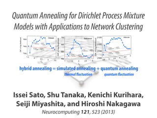
- 1. Quantum Annealing for Dirichlet Process Mixture Models with Applications to Network Clustering Issei Sato, Shu Tanaka, Kenichi Kurihara, Seiji Miyashita, and Hiroshi Nakagawa Neurocomputing 121, 523 (2013)
- 2. Main Results Diff. of log-likelihood Better We considered the efficiency of quantum annealing method for Dirichlet process mixture models. In this study, Monte Carlo simulation was performed. 21300 Wikivote 21200 21100 21000 2.5 3 3.5 4 4.5 5 0 - We constructed a method to apply quantum annealing to network clustering. - Quantum annealing succeeded to obtain a better solution than conventional methods. - The number of classes can be changed. (cf. K. Kurihara et al. and I. Sato et al., UAI2009) K. Kurihara et al., I. Sato et al., Proceedings of UAI2009.
- 3. Background Optimization problem To find the state (best solution) where the real-valued cost function is minimized. If the size of problem is small, we can easily obtain the best solution by brute-force calculation. However... if the size of problem is large, we cannot obtain the best solution by brute-force calculation in practice. We should develop methods to obtain the best solution (at least, better solution) efficiently.
- 4. Background Cost function of most optimization problems can be represented by Hamiltonian of classical discrete spin systems. We can use the knowledge of statistical physics. To find the state where the cost function is minimized. To find the ground state of the Hamiltonian. Simulated annealing (SA) By decreasing the temperature (thermal fluctuation) gradually, the ground state of the Hamiltonian is obtained. S. Kirkpatrick, C. D. Gelatte, and M. P. Vecchi, Science, 220, 671 (1983). SA can be adopted to both stochastic methods such as Monte Carlo method and deterministic method.
- 5. Background Quantum annealing (QA) By decreasing the quantum fluctuation gradually, the ground state of the Hamiltonian is obtained. T. Kadowaki and H. Nishimori, Phys. Rev. E, 58, 5355 (1998). E. Farhi, J. Goldstone, S. Gutmann, J. Lapan, A. Lundgren, and D. Preda, Science, 292, 472 (2001). G. E. Santoro, R. Martonak, E. Tosatti, and R. Car, Science, 295, 2427 (2002). Review articles G. E. Santoro and E. Tosatti, J. Phys. A: Math. Gen., 39, R393 (2006). A. Das and B. K. Chakrabarti, Rev. Mod. Phys., 80, 1061 (2008). S. Tanaka and R. Tamura, Kinki University Series on Quantum Computing Series "Lectures on Quantum Computing, Thermodynamics and Statistical Physics" (2012). QA is better than SA?
- 6. What is CRP?
- 7. Chinese Restaurant Process (CRP) Table (data class) Restaurant (entire set) 1 1 2 3 2 4 5 3 Customer (data point) Chinese Restaurant Process (CRP) assigns a probability for the seating arrangement of the customers.
- 8. Chinese Restaurant Process (CRP) Seating arrangement of the customers: Z = customer i sits at the k-th table: zi = k N {zi }i=1 N: the number of customers When customer i enters a restaurant with K occupied tables at which other customers are already seated, customer i sits at a table with the following probability: (k-th occupied table) +N 1 p(zi |Zzi ; ) Nk +N 1 (new unoccupied table) Nk: the number of customers sitting at the k-th table : hyper parameter of the CRP The log-likelihood of Z is given by p(Z) = K(Z) K(Z) N =1 (N + ) (Nk k=1 1)!
- 10. Quantum annealing for CRP (QACRP) QACRP uses multiple restaurants (m restaurants). customer i sits at the k-th table in the j-th restaurant: zj,i = k Seating arrangement of the customers in the j-th restaurant: Zj = {zj,i } In the j-th restaurant, when customer i enters a restaurant with K occupied tables at which other customers are already seated, customer i sits at a table with the following probability: Nj,k +N 1 /m (k-th occupied table) m pQA (zj,i | {Zd }d=1 {zj,i } ; , ) e (cj,k (i)+c+ (i))f ( , ) j,k /m +N 1 : inverse temperature (thermal fluctuation) : quantum fluctuation (new unoccupied table)
- 11. Quantum annealing for CRP (QACRP) /m Nj,k +N 1 e (cj,k (i)+c+ (i))f ( , ) j,k (k-th occupied table) m pQA (zj,i | {Zd }d=1 {zj,i } ; , ) /m (new unoccupied table) +N 1 c± (i) : the number of customers who sit at the k-th table in the j-th j,k restaurant and share tables with customer i in the (j ± 1)-th restaurant. j-1-th CRP 1 1 2 j+1-th CRP j-th CRP 3 2 4 5 3 1 1 4 3 2 5 3 2 1 3 4 1 2 5 2 The above fact will be proven in the following. 3
- 12. Quantum annealing for CRP (QACRP) Bit matrix representation for CRP A bit matrix B : adjacency matrix of customers 1 1 2 3 1 2 4 3 5 4 5 B Seating conditions ˜ 2 3 4 5 1 1 0 1 0 1 1 0 1 0 0 0 1 0 1 1 1 0 1 0 0 0 1 0 1 = N i=1 N n=1 ˜i,n Bi,n = Bn,i Bi,i = 1 (i = 1, 2, · · · , N ) i, , Bi /|Bi | · B /|B | = 1 or 0 Sitting arrangement can be represented by the Ising model with constraints.
- 13. Quantum annealing for CRP (QACRP) Bit matrix representation for CRP 1 1 2 4 3 2 2 1 2 1 1 0 1 0 0 customers who share a 1 0 table with customer 2. 1 4 3 3 4 5 5 1 1 1 1 0 1 0 0 1 0 0 0 1 1 0 1 1 0 1 0 0 1 0 0 0 0 0 0 a set of the states that customer 2 can take under the seating conditions. 3 4 5 1 1 0 1 0 1 1 0 1 0 0 0 1 0 1 1 1 0 1 0 0 0 1 0 1 1 1 5 2 2 3 4 5 1 0 1 0 0 1 0 1 0 1 0 1 0 1 0 1 2 3 4 5
- 14. Quantum annealing for CRP (QACRP) Density matrix representation for “classical” CRP Hc = diag[E( E( ( ) )= p( ) = (1) ), E( ln p( ( ) (2) ) + T e ), · · · E( ( ) T e Hc =: T ) )] ˜ ( ) Hc (2 N2 ˜ e Hc Zc Sitting arrangement can be represented by the Ising model with constraints.
- 15. Quantum annealing for CRP (QACRP) Formulation for quantum CRP H = Hc + Hq Hc : classical CRP Hq : quantum fluctuation T pQA ( ; , ) = Classical CRP p(˜i | ˜i ) = p(zi |Zzi ; ) e (Hc +Hq ) Te T ˜i e (Hc +Hq ) Hc T e Hc Nk +N 1 (k-th occupied table) +N 1 (new unoccupied table)
- 16. Quantum annealing for CRP (QACRP) Formulation for quantum CRP H = Hc + Hq Hc : classical CRP Hq : quantum fluctuation T pQA ( ; , ) = e (Hc +Hq ) Te Quantum CRP (Hc +Hq ) T pQA (˜i | ˜i ; , ) = ˜i e (Hc +Hq ) Te (Hc +Hq ) Transverse field as a quantum fluctuation N Hq = N x i,n , i=1 n=1 E= 1 0 0 1 , x = 0 1 1 0
- 17. Quantum annealing for CRP (QACRP) Approximation inference for QACRP T pQA ( ; , ) = e (Hc +Hq ) Te = (Hc +Hq ) pQA j (j ST ( , 2) 2, · · · m pQA ST ( 1 , 2, · · · , m; , )= N j+1 ) e , E( j=1 f ( , ) = 2 ln coth s( j , By the Suzuki-Trotter decomposition, pQA can be approximately expressed by the classical CRP. m; , )+O ef ( , )s( Z( , ) j )/m m N (˜j,i,n , ˜j+1,i,n ) = i=1 n=1 2N Z( , ) = sinh m e E( ) m 2 m j , j+1 )
- 18. Experiments Network model & dataset Citeseer citation network dataset for 2110 papers. 527 I. Sato et al. / Neurocomputing 121 (2013) 523–531 . (a) Social network (assortive network), (b) election network (disassortative network) and (c) citation network (mixture of assortative ning CRPs in which sj ðj ¼ 1; …; mÞ ment of the j-th CRP and represents ~ espond Bj;i;n ¼ 1 to s j;i;n ¼ ð1; 0Þ⊤ and means that we can represent Bj as the following121 (2013) 523–531 eurocomputing theorem: (10) is approximated by the Suzuki– ! β2 …; sm ; β; ΓÞ þ O ; m 1 e−β=mEðsj Þ ef ðβ;ΓÞsðsj ;sjþ1 Þ ; ¼ 1 Zðβ; ΓÞ ð15Þ m ∏ ð16Þ Netscience coauthorship network of regarded as a similarity function between the j-th and (j+1)-th bit matrices. If they are the same matrices, then sðs ; s Þ ¼ N . In scientists working on a network Eq. (2), log p ðs Þ corresponds to log e =Z and the regularizer term f Á Rðs ; …; s Þ is log ∏ e ¼ f ðβ; sðs ; s Þ. thatΓÞ∑ inference for scientists. has 1589 Note that we aim at deriving the approximation SA 1 −β=mEðsj Þ j m m f ðβ;ΓÞsðsj ;sjþ1 Þ j¼1 527 j 2 jþ1 m j¼1 j jþ1 pQA ðs i jss i ; β; ΓÞ in Eq. (13). Using Theorem 3.1, we can derive ~ ~ Eq. (4) as the approximation inference. The details of the derivation are provided in Appendix B. Wikivote a bipertite network constructed 4. Experiments using QA to a DPM We evaluated QA in a real application. We applied administrator elections. model for clustering vertices in a network where a seating 7115 Wikipedia users. arrangement of the CRP indicates a network partition. ples of network structures. (a) Social network (assortive network), (b) election network (disassortative network) and (c) citation network (mixture of assortative
- 19. Experiments Annealing schedule m : Trotter number, the number of replicas; m = 16 We tested several schedules of inverse temperature. ln(1 + t) 0 t 0t 0 = 0 = 0.2m, 0.4m, 0.6m t : t-th iteration. = 0.4m t is a better schedule in SA (MAP estimation). T = 0 m t is a schedule of quantum fluctuation. T : Total number of iterations
- 20. Diff. of log-likelihood Better Results 21300 Wikivote 21200 21100 21000 2.5 3 3.5 4 4.5 0 Lmax : the maximum log-likelihood of the beam search Beam Lmax : the maximum log-likelihood of 16 CRPs in SA 16SAs 5
- 21. Diff. of log-likelihood Results Citeseer 1600 1400 1200 Diff. of log-likelihood 1.5 2.5 3 Netscience We consider multiple running CRPs in which sj ðj ¼ 1; …; mÞ indicates the seating arrangement of the j-th CRP and represents ~ the j-th bit matrix Bj . We correspond Bj;i;n ¼ 1 to s j;i;n ¼ ð1; 0Þ⊤ and ⊤ Bj;i;n ¼ 0 to s j;i;n ¼ ð0; 1Þ , which means that we can represent Bj as ~ sj by using Eq. (5). We derive the following theorem: 600 500 1 Theorem 3.1. Sato ðs;al. ΓÞ in Eq. (10) is approximated by the Suzuki– I. pQA et β; / Neurocomputing 121 (2013) 523–531 Trotter expansion as2.5 follows: 3 1.5 2 0 pQA ðs; β; ΓÞ ¼ 21300 1 ⊤ −βðHc þHq Þ s e s Z Wikivote ¼ ∑ pQA−ST ðs; s2 ; …; sm ; β; ΓÞ þ O sj ðj≥2Þ 21200 2 ! β ; m pQA−ST ðs1 ; s2 ; …; sm ; β; ΓÞ 4. Experiments ð16Þ We evaluated QA in a real application. We applied QA to a DP model for clustering vertices in a network where a seati arrangement of the CRP indicates a network partition. 2.5 1 e−β=mEðsj Þ ef ðβ;ΓÞsðsj ;sjþ1 Þ ; Zðβ; ΓÞ j¼1 m ¼ ∏ regarded as a similarity function between the j-th and (j+1)-th matrices. If they are the same matrices, then sðsj ; sjþ1 Þ ¼ N 2 . Eq. (2), log pSA ðsj Þ corresponds to log e−β=mEðsj Þ =Z and the regulari term f Á Rðs1 ; …; sm Þ is log ∏m 1 ef ðβ;ΓÞsðsj ;sjþ1 Þ ¼ f ðβ; ΓÞ∑m 1 sðsj ; sjþ j¼ j¼ Note that we aim at deriving the approximation inference pQA ðs i jss i ; β; ΓÞ in Eq. (13). Using Theorem 3.1, we can der ~ ~ 527 Eq. (4) as the approximation inference. The details of the deriv tion are provided in Appendix B. ð15Þ where we rewrite s as s1 , and 21100 21000 I. Sato et al. / Neurocomputing 121 (2013) 523–531 3.5 Fig. 5. Examples of network structures. (a) Social network (assortive network), (b) election network (disassortative network) and (c) citation network (mixture of assorta and disassortative network). 0 700 400 Diff. of log-likelihood 2 Better solution can be obtained by QA. β Γ ; ð17Þ f ðβ; ΓÞ ¼ 2 Fig. 5. Examples of network structures. (a) Social network (assortive network), (b) election network (disassortative network) and (c) citation netwo log coth m 4.1. Network model and disassortative network). 3 3.5 4 N 4.5 5 N ~ ~ sðsj ; sjþ1 Þ ¼ 0∑ ∑ δðs j;i;n ; s jþ1;i;n Þ; ð18Þ We used the Newman model [17] for network modeling in t
- 22. Diff. of log-likelihood Results Citeseer 1600 SA(T=30,m=1) 13 sec. calc. time QA(T=30,m=16) 15 sec. 1400 16 SAs 1200 1600 SAs beam search QA(m=16) 35 30 57 37 # classes 1.5 2 2.5 3 3.5 Diff. of log-likelihood 0 700 SA(T=30,m=1) calc. time 600 25 sec. 16 SAs 500 400 QA(T=30,m=16) 22 sec. Netscience 1600 SAs beam search QA(m=16) 22 65 61 26 # classes 1 1.5 2 2.5 3 Diff. of log-likelihood 0 21300 SA(T=30,m=1) calc. time 21200 79 sec. 16 SAs 21100 21000 QA(T=30,m=16) 76 sec. Wikivote # classes 2.5 3 3.5 4 0 4.5 5 1600 SAs beam search QA(m=16) 8 8 27 8
- 23. Main Results Diff. of log-likelihood Better We considered the efficiency of quantum annealing method for Dirichlet process mixture models. In this study, Monte Carlo simulation was performed. 21300 Wikivote 21200 21100 21000 2.5 3 3.5 4 4.5 5 0 - We constructed a method to apply quantum annealing to network clustering. - Quantum annealing succeeded to obtain a better solution than conventional methods. - The number of classes can be changed. (cf. K. Kurihara et al. and I. Sato et al., UAI2009) K. Kurihara et al., I. Sato et al., Proceedings of UAI2009.
- 24. Thank you ! Issei Sato, Shu Tanaka, Kenichi Kurihara, Seiji Miyashita, and Hiroshi Nakagawa Neurocomputing 121, 523 (2013)