SlideShare ist ein Scribd-Unternehmen logo
1 von 22
Null Hypothesis: The use of knives in domestic violence incidents has significantly
                                                                changed during 1994 and 1995.

                                                               Research Hypothesis: The use of knives in domestic violence incidents has not
                                                               changed during 1994 and 1995.

                                 Our hypothesis is drawn from a sampling that observed 1994 and 1995 aggravated and non-aggravated assault
                                 charges drawn from the Statistical Crime Data for the State of Maryland, c. 1995. The one-way chi-test can be used
to determine whether the frequencies observed differs significantly from an even distribution (or any other distribution hypothesized).

What should the frequency distribution of correct observances look like if the null hypothesis were true? The charts below demonstrate two
categories with the anticipation that 50% of the reported results should fall in each classification. With 20.378 incidents for 1994 and 24.021 for
1995, we should expect 4.08 occurrences (in 1994) and 4.80 occurrences (in 1995) in each Type of Weapon Category. The expected frequencies are
those frequencies that are expected to occur under the term of the Null Hypothesis.


1994 (In Hundreds)              fo                      fe                    fo - fe               (fo - fe)2              (fo - fe)2
Type of Weapons                                                                                                                 fe

Firearm                        .272                    4.08                   -3.80                  14.44                    3.5

Knife                          .849                    4.08                   -3.23                  10.43                    2.6

Other Dangerous               1.423                    4.08                   -2.66                   7.08                    1.7
Weapons

Hands, Fists, Feet,            .667                    4.08                   -3.41                  11.63                    2.9
etc.

Non-Aggravated                17.167                   4.08                   13.09                  171.3                    41.9

              Total           20.378                                                                                          52.6

1995 (In Hundreds)              fo                      fe                    fo - fe               (fo - fe)2              (fo - fe)2
Type of Weapons                                                                                                                 fe

Firearm                        .252                    4.80                   -2.28                   5.19                    1.1
Knife                          1.074                   4.80                         -3.73               13.91                  2.9

Other Dangerous                1.771                   4.80                         -3.03                9.18                  1.9
Weapons

Hands, Fists, Feet,            .672                    4.80                         -4.13               17.06                  3.6
etc.

Non-Aggravated                20.252                   4.80                         15.45               238.70                49.7

              Total           24.021                                                                                          59.2


                               Null Hypothesis: The use of knives in domestic violence incidents has significantly changed during 1994 and 1995.

                              Research Hypothesis: The use of knives in domestic violence incidents has not changed during 1994 and 1995.

                                                                     (Continued)

The chi-squared method allows us to test the significance of the difference between a set of observed frequencies and expected frequencies.

Based on just the observed and expected frequencies, the formula for chi-square is:

                                                                       (fo - fe)2

                                                                       X2 = Σ fe

where fo = observed frequency in any category

fe = expected frequency in any category

Our next step is to interpret the chi-square value by determining the appropriate degrees of freedom.

                                                                      df = k - 1

where k = number of categories in the observed frequency distribution. Our example shows 5 categories (firearms; knives; other dangerous weapons;
hands, fists, feet, etc.; and non-aggravated) in 1994 and 1995:
df = 5 - 1 = 4

Now by checking The Critical Value of Chi-Square at the .05 and .01 Chart, we look for the .05 significant level to check 4 degrees of freedom. The
value is 9.488. This is the value that we must exceed before we can reject the null hypothesis. Because our calculated chi-square for 1994 is 52.6 and
for 1995 is 59.2, it is larger than the table value, we reject the null hypothesis and accept the research hypothesis. The observed frequencies do differ
significantly from the expected occurrence for an equal distribution under the null hypothesis for knife usage in domestic violence situations.

                 In comparing the chi-squared test to our obtained frequencies, the reported sampling did not indicate a perfectly even distribution
                 (4.08 in 1994 and 4.80 in 1995 for each type of weapon), the degree of unevenness was sufficiently large.

                                       Null Hypothesis: Unknown factors do not play a significant role in
                                       domestic violence occurrences during 1994 and 1995.
                                       Research Hypothesis: Unknown factors do play a significant role in
                                       domestic violence occurrences during 1994 and 1995.
This hypothesis was also taken from a sampling that observed 1994 and 1995 unknown factors in
domestic violence drawn from The Statistical Crime Data for the State of Maryland, c. 1995.
Again, the one-way chi-test will be used to determine whether the frequencies observed differs
significantly from an even distribution (or any other distribution hypothesized).
We want to demonstrate if this frequency distribution for unknown factors shows if the null
hypothesis is true? The charts below demonstrate two categories with the anticipation that 50% of
the reported results should fall in each classification. With 20.378 incidents for 1994 and 24.021
incidents for 1995, we should expect .926 occurrences (in 1994) and 1.091 occurrences (in 1995)
for each year’s Circumstances Category. The expected frequencies are those incidents that are
expected to occur under the term of the Null Hypothesis.

1994 (In                      fo                    fe                  fo - fe                     (fo - fe)2                    (fo - fe)2
Hundreds)
Circumstances                                    fe

Alcohol          2.686   .926   1.76     3.098   3.4

Drugs            .373    .926   -0.553   .306    .3

Food/Cooking     .100    .926   -0.826   .682    .7

Friends          .169    .926   -0.757   .573    .6

Gambling         .005    .926   -0.921   .848    .9

Household        .128    .926   -0.798   .637    .7
Chores

Infidelity       1.055   .926   0.129    .017    0

Employment/Job   .104    .926   -0.822   .676    .7

Mental           .090    .926   -0.836   .699    .8
Imbalance

Money            .817    .926   -0.109   .012    0

Children         .914    .926   -0.012   1.44    1.6

Property         .609    .926   -0.317   .100    .1

Relative         .114    .926   -0.812   .659    .7

Sex              .168    .926   -0.758   .575    .6

Hobby            .011    .926   -0.915   .837    .9

T.V.             .054    .926   -0.872   .760    .8
Separation            .628    .926    -0.298                  .089                  .1

Divorce               .129    .926    -0.797                  .635                  .7

Reconciliation        .030    .926    -0.896                  .803                  .9

Out Late              .398    .926    -0.528                  .279                  .3

Other                3.716    .926    2.79                   7.784                 8.4

Unknown              8.080    .926    7.154                  51.180                55.3

             Total   20.378                                                        78.5

1995 (In               fo      fe     fo - fe   (fo - fe)2            (fo - fe)2
Hundreds)
                                                                          fe
Circumstances

Alcohol              3.139    1.091   2.048      4.194                  3.8

Drugs                 .458    1.091   -.633      .401                    .4

Food/Cooking          .163    1.091   -.928      .861                    .8

Friends               .278    1.091   -.813      .661                    .6

Gambling              .012    1.091   -1.079     1.164                   .1

Household             .162    1.091   -.929      .863                    .8
Chores

Infidelity           1.372    1.091   .281       .079                    .1

Employment/Job        .122    1.091   -.969      .939                    .9
Mental                .110          1.091         -.981         .962                .9
Imbalance

Money                1.043          1.091          .048         2.304               2.1

Children             1.181          1.091          .09           8.1                7.4

Property              .963          1.091         -.128         .016                .0

Relative              .202          1.091         -.889         .790                1.4

Sex                   .224          1.091         -.867         .752                .7

Hobby                 .011          1.091         -1.08         1.166               .1

T.V.                  .061          1.091         -1.03         1.061               .9

Separation            .901          1.091          .19          .036                .0

Divorce               .162          1.091          .929         .863                .8

Reconciliation        .037          1.091         1.054         1.111               1.0

Out Late              .510          1.091         -.581         .338                .3

Other                2.877          1.091         1.786         3.190               2.9

Unknown              10.033         1.091         8.942         79.96              73.29

             Total   24.021                                                       101.29


                              Null Hypothesis: Unknown factors do not play a significant role in
                              domestic violence occurrences during 1994 and 1995.
Research Hypothesis: Unknown factors do play a significant role in
                                      domestic violence occurrences during 1994 and 1995.
                                                                     (Continued)

The chi-squared method allows us to test the significance of the difference between a set of observed frequencies and expected frequencies.

Based on just the observed and expected frequencies, the formula for chi-square is:

                                                                        (fo - fe)2

                                                                       X2 = Σ fe

where fo = observed frequency in any category

fe = expected frequency in any category

Our next step is to interpret the chi-square value by determining the appropriate degrees of freedom.

                                                                       df = k - 1

where k = number of categories in the observed frequency distribution. Our example shows 22 categories (Alcohol, Drugs, Food/Cooking, Friends,
Gambling, Household Chores, Infidelity, Employment/Job, Mental Imbalance, Money, Children, Property, Relative, Sex, Hobby, T.V., Separation,
Divorce, Reconciliation, Out Late, Other and Unknown) in 1994 and 1995:

                                                                   df = 22 - 1 = 21

Now by checking The Critical Value of Chi-Square at the .05 and .01 Chart, we look for the .05 significant level to check 21 degrees of freedom. The
value is 32.671. This is the value that we must exceed before we can reject the null hypothesis. Because our calculated chi-square for 1994 is 78.5
and for 1995 is 101.29, it is larger than the table value, we reject the null hypothesis and accept the research hypothesis. The observed frequencies do
differ significantly from the expected occurrence for an equal distribution under the null hypothesis for unknown factors in domestic violence
situations.

In comparing the chi-squared test to our obtained frequencies, the reported sampling did not indicate a perfectly even distribution (.926 in 1994 and
1.091 in 1995 for each circumstance), the degree of unevenness was sufficiently large.
Null Hypothesis: The morning hours have an effect on domestic violence
                            during 1994 and 1995.
                            Research Hypothesis: The morning hours have no effect on domestic
                            violence during 1994 and 1995.
The above hypothesis was also taken from a sampling that observed domestic violence’s 1994 and
1995 incidents occurring in the morning hours. This sample was also drawn from The Statistical
Crime Data for the State of Maryland, c. 1995. Again, the one-way chi-test will be used to
determine whether the frequencies observed differs significantly from an even distribution (or any
other distribution hypothesized).
We want to demonstrate if this frequency distribution for the morning hours shows if the null
hypothesis is true? The charts below demonstrate two categories with the anticipation that 50% of
the reported results should fall in each classification. With 76.95 incidents for 1994 and 93.57
incidents for 1995, we should expect 6.41 morning occurrences (in 1994) and 7.80 morning
occurrences (in 1995) for each year’s Morning Hours Category. The expected frequencies are those
incidents that are expected to occur under the term of the Null Hypothesis.

1994 (In Hundreds)    fo               fe            fo - fe        (fo - fe)2     (fo - fe)2

Morning Hours                                                                          fe

12:00 A.M.           9.85             6.41           3.44            11.83           1.8

1:00 A.M.            10.6             6.41           4.19            17.56           2.7

2:00 A.M.            8.34             6.41           1.93            3.72             .6

3:00 A.M.            6.38             6.41            -.03              9            1.4
4:00 A.M.            4.33    6.41   -2.08      4.33           .7

5:00 A.M.            2.92    6.41   -3.49      12.18         1.9

6:00 A.M.            3.22    6.41   -3.19      10.17         1.6

7:00 A.M.            3.29    6.41   -3.12      9.73          1.5

8:00 A.M.            4.58    6.41   -1.83      3.35           .5

9:00 A.M.            5.92    6.41   -.49        .24           .0

10:00 A.M.           7.91    6.41    1.5       2.25           .4

11:00 A.M.           9.61    6.41    3.2       10.24         1.6

             Total   76.95                                  14.7

1995 (In Hundreds)    fo      fe    fo - fe   (fo - fe)2   (fo - fe)2

Morning Hours                                                  fe

12:00 A.M.           12.89   7.8    5.09       25.9          3.3

1:00 A.M.            13.17   7.8    5.37       28.8          3.7

2:00 A.M.            10.7    7.8     2.9       8.41          1.1

3:00 A.M.            8.02    7.8     .22        .04          5.1

4:00 A.M.            4.97    7.8    -2.83         8            1

5:00 A.M.            3.79    7.8    -4.01        16          2.1

6:00 A.M.            3.44    7.8    -4.36        19          2.4
7:00 A.M.                       4.17                     7.8                    -3.63                  13.2                   1.7

                8:00 A.M.                       5.45                     7.8                    -2.35                  5.52                    .7

                9:00 A.M.                       7.22                     7.8                     -.58                   .34                    0

                10:00 A.M.                      9.34                     7.8                    1.54                   2.37                    .3

                11:00 A.M.                      10.41                    7.8                    2.61                   6.81                    .9

                               Total            93.57                                                                                         22.3


                                       Null Hypothesis: The morning hours have an effect on domestic violence
                                       occurrences during 1994 and 1995.
                                       Research Hypothesis: The morning hours have no effect on domestic
                                       violence occurrences during 1994 and 1995.
                                                                     (Continued)

The chi-squared method allows us to test the significance of the difference between a set of observed frequencies and expected frequencies.

Based on just the observed and expected frequencies, the formula for chi-square is:

                                                                       (fo - fe)2

                                                                       X2 = Σ fe

where fo = observed frequency in any category

fe = expected frequency in any category

Our next step is to interpret the chi-square value by determining the appropriate degrees of freedom.
df = k - 1

where k = number of categories in the observed frequency distribution. Our example shows 12 categories (from 12:00 a.m. until 11:00 a.m.) in 1994
and 1995:

                                                                   df = 12 - 1 = 11

Now by checking The Critical Value of Chi-Square at the .05 and .01 Chart, we look for the .05 significant level to check 11 degrees of freedom. The
value is 19.675. This is the value that we must exceed before we can reject the null hypothesis. Because our calculated chi-square for 1994 is 14.7
and for 1995 is 22.3, it is smaller than the table value, we accept the null hypothesis and reject the research hypothesis. The observed frequencies do
not differ significantly from the expected occurrence for an equal distribution under the null hypothesis for morning incidents in domestic violence
situations.

In comparing the chi-squared test to our obtained frequencies, the reported sampling did indicate a perfectly even distribution (6.41 in 1994 and 7.8
in 1995 for each circumstance) for the Morning Hours Category in 1994. However, comparing the chi-squared test to our obtained frequencies for the
Morning Hours Category in 1995, the reported sampling did not indicate a perfectly even distribution (6.41 in 1994 and 7.8 in 1995 for each
circumstance) the degree of unevenness was significantly large.

                                      Null Hypothesis: The afternoon hours have an effect on domestic
                                      violence occurrences during 1994 and 1995.
                                      Research Hypothesis: The afternoon hours have no affect on domestic
                                      violence occurrences during 1994 and 1995.
The above hypothesis was also taken from a sampling that observed domestic violence 1994 and
1995 incidents occurring in the afternoon hours. This sample was also drawn from The Statistical
Crime Data for the State of Maryland, c. 1995. Again, the one-way chi-test will be used to
determine whether the frequencies observed differs significantly from an even distribution (or any
other distribution hypothesized).
We want to demonstrate if this frequency distribution for the afternoon hours shows if the null
hypothesis is true? The charts below demonstrate two categories with the anticipation that 50% of
the reported results should fall in each classification. With 76.95 incidents for 1994 and 93.57
incidents for 1995, we should expect 5 morning occurrences (in 1994) and 6 morning occurrences
(in 1995) for each year’s Afternoon Hours Category. The expected frequencies are those incidents
that are expected to occur under the term of the Null Hypothesis.

1994 (In Hundreds)    fo             fe            fo - fe        (fo - fe)2      (fo - fe)2

Afternoon Hours                                                                       fe

12:00 P.M.           8.17          10.57           -2.4            5.76              .5

1:00 P.M.            6.79          10.57           -3.78           14.29            1.4

2:00 P.M.            9.43          10.57           -1.14            1.3              .1

3:00 P.M.            9.89          10.57           -.068            .46               0

4:00 P.M.            9.99          10.57           -.58             .34               0

5:00 P.M.            8.87          10.57           -1.7            2.89              .3

6:00 P.M.             10           10.57           -.57             .32               0

7:00 P.M.            11.58         10.57           1.01            1.02              .1

8:00 P.M.            11.93         10.57           1.36            1.85              .2

9:00 P.M.            12.57         10.57             2                4              .4

10:00 P.M.           13.98         10.57           3.41            11.63            1.1

11:00 P.M.           13.63         10.57           3.06            9.36              .9

             Total   76.95                                                            5

1995 (In Hundreds)    fo             fe            fo - fe        (fo - fe)2      (fo - fe)2
Afternoon Hours

                                                                                       fe

12:00 P.M.           10.42              12.22           -1.8           25.9            .3

1:00 P.M.             8.09              12.22          -4.13           28.8           1.4

2:00 P.M.            10.05              12.22          -2.17           8.41            .4

3:00 P.M.            10.66              12.22          -1.56           .04             .2

4:00 P.M.            10.43              12.22          -1.79            8              .3

5:00 P.M.            10.05              12.22          -2.17           16              .4

6:00 P.M.            11.61              12.22           -.61           19              0

7:00 P.M.            13.21              12.22           .99            13.2            0

8:00 P.M.            14.34              12.22           2.12           5.52            .4

9:00 P.M.            15.23              12.22           3.01           .34             .7

10:00 P.M.           16.08              12.22           3.86           2.37           1.2

11:00 P.M.           16.47              12.22           4.25           6.81            .7

             Total   146.64                                                            6

                              Null Hypothesis: The afternoon hours have an effect on domestic
                              violence occurrences during 1994 and 1995.
                              Research Hypothesis: The afternoon hours have no effect on domestic
                              violence occurrences during 1994 and 1995.
(Continued)

The chi-squared method allows us to test the significance of the difference between a set of observed frequencies and expected frequencies.

Based on just the observed and expected frequencies, the formula for chi-square is:

                                                                       (fo - fe)2

                                                                       X2 = Σ fe

where fo = observed frequency in any category

fe = expected frequency in any category

Our next step is to interpret the chi-square value by determining the appropriate degrees of freedom.

                                                                      df = k - 1

where k = number of categories in the observed frequency distribution. Our example shows 12 categories (from 12:00 p.m. through 11:00 p.m.) in
1994 and 1995:

                                                                   df = 12 - 1 = 11

Now by checking The Critical Value of Chi-Square at the .05 and .01 Chart, we look for the .05 significant level to check 11 degrees of freedom. The
value is 19.675. This is the value that we must exceed before we can reject the null hypothesis. Because our calculated chi-square for 1994 is 5 and
for 1995 is 6, it is smaller than the table value, we accept the null hypothesis and reject the research hypothesis. The observed frequencies do not
differ significantly from the expected occurrence for an equal distribution under the null hypothesis for morning incidents in domestic violence
situations.

In comparing the chi-squared test to our obtained frequencies, the reported sampling did indicate a perfectly even distribution (10.57 in 1994 and
12.22 in 1995 for each circumstance).

                                      Null Hypothesis: The months of the year have an effect on domestic
                                      violence during 1994 and 1995.
Research Hypothesis: The months of the year have no affect on domestic
                             violence during 1994 and 1995.
The above hypothesis was also taken from a sampling that observed domestic violence 1994 and
1995 incidents occurring in the month of the year. This sample was also drawn from The Statistical
Crime Data for the State of Maryland, c. 1995. Again, the one-way chi-test will be used to
determine whether the frequencies observed differs significantly from an even distribution (or any
other distribution hypothesized).
We want to demonstrate if this frequency distribution for the month of the year shows if the null
hypothesis is true? The charts below demonstrate two categories with the anticipation that 50% of
the reported results should fall in each classification. With 20.378 incidents for 1994 and 24.021
incidents for 1995, we should expect 1.7 monthly occurrences (in 1994) and 2 monthly occurrences
(in 1995) for each of the year’s Month of the Year Category. The expected frequencies are those
incidents that are expected to occur under the term of the Null Hypothesis.

1994 (In Hundreds)    fo                fe            fo - fe       (fo - fe)2      (fo - fe)2

Month of Year                                                                           fe

January              1.542              1.7           -.158           .03            .014

February             1.486              1.7           -.214           .05            .027

March                1.734              1.7           .034           .001               0

April                1.710              1.7            .01              0               0

May                  1.690              1.7           -.01              0               0
June                 1.705    1.7   .005          0            0

July                 1.822    1.7   .122        .01            0

August               1.812    1.7   .112        .01            0

September            1.834    1.7   .134        .02            0

October              1.804    1.7   .104        .01            0

November             1.666    1.7   .034       .001            0

December             1.573    1.7   .127        .02            0

            Total    20.378                                 .041

1995 (In Hundreds)     fo     fe    fo - fe   (fo - fe)2   (fo - fe)2

Month of Year                                                  fe

January              1.937    2     -.063      .001         .005

February             1.526    2     -.474      .224         .112

March                1.941    2     -.059      .002         .001

April                1.906    2     -.094      .001         .005

May                  2.128    2     .128        .02          .01

June                 2.046    2     .046       2.12         1.06

July                 2.277    2     .277        .08         .139

August               2.181    2     .181        .03         .015
September                      2.003                     2                          .003                 0                      0

October                        1.986                     2                          -.014                0                      0

November                       1.918                     2                          -.082               .006                  .003

December                       2.172                     2                          .172                .029                  .015

              Total           24.021                                                                                          1.365

                                       Null Hypothesis: The months of the year have an effect on domestic
                                       violence during 1994 and 1995.
                                       Research Hypothesis: The months of the year have no effect on domestic
                                       violence during 1994 and 1995.
                                                                     (Continued)

The chi-squared method allows us to test the significance of the difference between a set of observed frequencies and expected frequencies.

Based on just the observed and expected frequencies, the formula for chi-square is:

                                                                       (fo - fe)2

                                                                       X2 = Σ fe

where fo = observed frequency in any category

fe = expected frequency in any category

Our next step is to interpret the chi-square value by determining the appropriate degrees of freedom.

                                                                      df = k - 1

where k = number of categories in the observed frequency distribution. Our example shows 12 categories (from January through December) in 1994
and 1995:
df = 12 - 1 = 11

Now by checking The Critical Value of Chi-Square at the .05 and .01 Chart, we look for the .05 significant level to check 11 degrees of freedom. The
value is 19.675. This is the value that we must exceed before we can reject the null hypothesis. Because our calculated chi-square for 1994 is .041
and for 1995 is 1.365, it is smaller than the table value, we accept the null hypothesis and reject the research hypothesis. The observed frequencies do
not differ significantly from the expected occurrence for an equal distribution under the null hypothesis for monthly incidents in domestic violence
situations.

In comparing the chi-squared test to our obtained frequencies, the reported sampling did indicate a perfectly even distribution (1.7 in 1994 and 2 in
1995 for each circumstance).

                                      Null Hypothesis: The day of the week has an affect on domestic violence
                                      occurring in 1994 and 1995.
                                      Research Hypothesis: The day of the week has no effect on domestic
                                      violence occurring in 1994 and 1995.
The above hypothesis was also taken from a sampling that observed domestic violence 1994 and
1995 incidents occurring on a certain day of the week. This sample was also drawn from The
Statistical Crime Data for the State of Maryland, c. 1995. Again, the one-way chi-test will be used
                to determine whether the frequencies observed differs significantly from an even
                distribution (or any other distribution hypothesized).
                We want to demonstrate if this frequency distribution for the day of the week shows
                if the null hypothesis is true? The charts below demonstrate two categories with the
                anticipation that 50% of the reported results should fall in each classification. With
20.378 incidents for 1994 and 24.021 incidents for 1995, we should expect 2.911 monthly
occurrences (in 1994) and 3.432 monthly occurrences (in 1995) for each of the year’s Day of the
Week Category. The expected frequencies are those incidents that are expected to occur under the
term of the Null Hypothesis.
1994 (In Hundreds)      fo      fe     fo - fe   (fo - fe)2   (fo - fe)2

Day of Week                                                       fe

Monday                3.017    2.911   .106       .011         .003

Tuesday               2.703    2.911   -.208      .043         .015

Wednesday             2.457    2.911   -.454      .206          .07

Thursday              2.479    2.911   -.432      .187         ..064

Friday                2.846    2.911   -.065      .004         .001

Saturday              3.290    2.911   .379       .144         .049

Sunday                3.586    2.911   .675       .456         .157

              Total   20.378                                   .359

1995 (In Hundreds)      fo      fe     fo - fe   (fo - fe)2   (fo - fe)2

Day of Week                                                       fe

Monday                3.322    3.432   -.11       .012          3.5

Tuesday               3.246    3.432   -.186      .346          .01

Wednesday             3.019    3.432   -.413      .171          .05

Thursday              2.956    3.432   -.476      .227          .07

Friday                3.207    3.432   -.225      .051          .01

Saturday              3.980    3.432   .548         .3          .08
Sunday                         4.291                   3.432                     .859                   .738                      .02

              Total           24.021                                                                                             3.74

                                       Null Hypothesis: The day of the week has an effect on domestic violence
                                       occurring in 1994 and 1995.
                                       Research Hypothesis: The day of the week has no effect on domestic
                                       violence occurring in 1994 and 1995.
                                                                     (Continued)

The chi-squared method allows us to test the significance of the difference between a set of observed frequencies and expected frequencies.

          Based on just the observed and expected frequencies, the formula for chi-square is:

                                                                             (fo - fe)2

                                                                             X2 = Σ fe

where fo = observed frequency in any category

fe = expected frequency in any category

Our next step is to interpret the chi-square value by determining the appropriate degrees of freedom.

                                                                       df = k - 1

where k = number of categories in the observed frequency distribution. Our example shows 7 categories (from Monday through Sunday) in 1994 and
1995:

                                                                     df = 7 - 1 = 6

Now by checking The Critical Value of Chi-Square at the .05 and .01 Chart, we look for the .05 significant level to check 6 degrees of freedom. The
value is 12.592. This is the value that we must exceed before we can reject the null hypothesis. Because our calculated chi-square for 1994 is .359
and for 1995 is 3.74, it is smaller than the table value, we accept the null hypothesis and reject the research hypothesis. The observed frequencies do
not differ significantly from the expected occurrence for an equal distribution under the null hypothesis for day of the week incidents in domestic
violence situations.

In comparing the chi-squared test to our obtained frequencies, the reported sampling did indicate a perfectly even distribution (2.911 in 1994 and
3.432 in 1995 for each circumstance).

                                     INTRODUCTION
The act of domestic violence has no label. It could happen to any gender, at any age and
in any occupation. Domestic violence can also take on the form of mental, physical,
verbal, emotional, and psychological abuse. The ultimate goal of a domestic violence
abuser is to have total control and power over another person. This situation can be
inflicted upon anyone at anytime. Russell Hovan’s perspective states, “There are
situations in life to which the only satisfactory response is a physically violent one. If you
don’t make that response, you continually relive the unresolved situation over and over in
your life.” (b. 1925, U.S. author. Novelists in Interview (ed. by John Haffenden, 1985)).
The scariest account of domestic violence occurs when you do not have to see a scar to
feel one. It’s like a thief in the night, because we don’t think about it until it indirectly or
directly affects us on a personal level. There are many cases that have unknown causes
and probably as many that go unreported. It’s a time bomb waiting to explode, and we will
show the impact of the explosion by reviewing 1994 and 1995 domestic violence data.
Our source was provided through the publication, The Statistical Crime Data for the State
of Maryland. By using the chi-squared test, it will demonstrate if there is a significant or
insignificant trend.
CONCLUSION
As the data shows, domestic violence in the State of Maryland for 1994 and 1995
indicates it is on the rise. We must all take steps to neutralize this time bomb. Because
everybody is a victim as long as the abuse continues. In addition, everyone must begin to
take an active and responsible role to curve this silent offense. As long as we continue to
allow these abuses to perpetuate, we are threatening our own futures. If the trend
continues to rise as it has been reported in 1994 and 1995, our children’s behaviors may
grow more vicious in nature.

Weitere ähnliche Inhalte

Empfohlen

AI Trends in Creative Operations 2024 by Artwork Flow.pdf
AI Trends in Creative Operations 2024 by Artwork Flow.pdfAI Trends in Creative Operations 2024 by Artwork Flow.pdf
AI Trends in Creative Operations 2024 by Artwork Flow.pdfmarketingartwork
 
PEPSICO Presentation to CAGNY Conference Feb 2024
PEPSICO Presentation to CAGNY Conference Feb 2024PEPSICO Presentation to CAGNY Conference Feb 2024
PEPSICO Presentation to CAGNY Conference Feb 2024Neil Kimberley
 
Content Methodology: A Best Practices Report (Webinar)
Content Methodology: A Best Practices Report (Webinar)Content Methodology: A Best Practices Report (Webinar)
Content Methodology: A Best Practices Report (Webinar)contently
 
How to Prepare For a Successful Job Search for 2024
How to Prepare For a Successful Job Search for 2024How to Prepare For a Successful Job Search for 2024
How to Prepare For a Successful Job Search for 2024Albert Qian
 
Social Media Marketing Trends 2024 // The Global Indie Insights
Social Media Marketing Trends 2024 // The Global Indie InsightsSocial Media Marketing Trends 2024 // The Global Indie Insights
Social Media Marketing Trends 2024 // The Global Indie InsightsKurio // The Social Media Age(ncy)
 
Trends In Paid Search: Navigating The Digital Landscape In 2024
Trends In Paid Search: Navigating The Digital Landscape In 2024Trends In Paid Search: Navigating The Digital Landscape In 2024
Trends In Paid Search: Navigating The Digital Landscape In 2024Search Engine Journal
 
5 Public speaking tips from TED - Visualized summary
5 Public speaking tips from TED - Visualized summary5 Public speaking tips from TED - Visualized summary
5 Public speaking tips from TED - Visualized summarySpeakerHub
 
ChatGPT and the Future of Work - Clark Boyd
ChatGPT and the Future of Work - Clark Boyd ChatGPT and the Future of Work - Clark Boyd
ChatGPT and the Future of Work - Clark Boyd Clark Boyd
 
Getting into the tech field. what next
Getting into the tech field. what next Getting into the tech field. what next
Getting into the tech field. what next Tessa Mero
 
Google's Just Not That Into You: Understanding Core Updates & Search Intent
Google's Just Not That Into You: Understanding Core Updates & Search IntentGoogle's Just Not That Into You: Understanding Core Updates & Search Intent
Google's Just Not That Into You: Understanding Core Updates & Search IntentLily Ray
 
Time Management & Productivity - Best Practices
Time Management & Productivity -  Best PracticesTime Management & Productivity -  Best Practices
Time Management & Productivity - Best PracticesVit Horky
 
The six step guide to practical project management
The six step guide to practical project managementThe six step guide to practical project management
The six step guide to practical project managementMindGenius
 
Beginners Guide to TikTok for Search - Rachel Pearson - We are Tilt __ Bright...
Beginners Guide to TikTok for Search - Rachel Pearson - We are Tilt __ Bright...Beginners Guide to TikTok for Search - Rachel Pearson - We are Tilt __ Bright...
Beginners Guide to TikTok for Search - Rachel Pearson - We are Tilt __ Bright...RachelPearson36
 
Unlocking the Power of ChatGPT and AI in Testing - A Real-World Look, present...
Unlocking the Power of ChatGPT and AI in Testing - A Real-World Look, present...Unlocking the Power of ChatGPT and AI in Testing - A Real-World Look, present...
Unlocking the Power of ChatGPT and AI in Testing - A Real-World Look, present...Applitools
 
12 Ways to Increase Your Influence at Work
12 Ways to Increase Your Influence at Work12 Ways to Increase Your Influence at Work
12 Ways to Increase Your Influence at WorkGetSmarter
 

Empfohlen (20)

AI Trends in Creative Operations 2024 by Artwork Flow.pdf
AI Trends in Creative Operations 2024 by Artwork Flow.pdfAI Trends in Creative Operations 2024 by Artwork Flow.pdf
AI Trends in Creative Operations 2024 by Artwork Flow.pdf
 
Skeleton Culture Code
Skeleton Culture CodeSkeleton Culture Code
Skeleton Culture Code
 
PEPSICO Presentation to CAGNY Conference Feb 2024
PEPSICO Presentation to CAGNY Conference Feb 2024PEPSICO Presentation to CAGNY Conference Feb 2024
PEPSICO Presentation to CAGNY Conference Feb 2024
 
Content Methodology: A Best Practices Report (Webinar)
Content Methodology: A Best Practices Report (Webinar)Content Methodology: A Best Practices Report (Webinar)
Content Methodology: A Best Practices Report (Webinar)
 
How to Prepare For a Successful Job Search for 2024
How to Prepare For a Successful Job Search for 2024How to Prepare For a Successful Job Search for 2024
How to Prepare For a Successful Job Search for 2024
 
Social Media Marketing Trends 2024 // The Global Indie Insights
Social Media Marketing Trends 2024 // The Global Indie InsightsSocial Media Marketing Trends 2024 // The Global Indie Insights
Social Media Marketing Trends 2024 // The Global Indie Insights
 
Trends In Paid Search: Navigating The Digital Landscape In 2024
Trends In Paid Search: Navigating The Digital Landscape In 2024Trends In Paid Search: Navigating The Digital Landscape In 2024
Trends In Paid Search: Navigating The Digital Landscape In 2024
 
5 Public speaking tips from TED - Visualized summary
5 Public speaking tips from TED - Visualized summary5 Public speaking tips from TED - Visualized summary
5 Public speaking tips from TED - Visualized summary
 
ChatGPT and the Future of Work - Clark Boyd
ChatGPT and the Future of Work - Clark Boyd ChatGPT and the Future of Work - Clark Boyd
ChatGPT and the Future of Work - Clark Boyd
 
Getting into the tech field. what next
Getting into the tech field. what next Getting into the tech field. what next
Getting into the tech field. what next
 
Google's Just Not That Into You: Understanding Core Updates & Search Intent
Google's Just Not That Into You: Understanding Core Updates & Search IntentGoogle's Just Not That Into You: Understanding Core Updates & Search Intent
Google's Just Not That Into You: Understanding Core Updates & Search Intent
 
How to have difficult conversations
How to have difficult conversations How to have difficult conversations
How to have difficult conversations
 
Introduction to Data Science
Introduction to Data ScienceIntroduction to Data Science
Introduction to Data Science
 
Time Management & Productivity - Best Practices
Time Management & Productivity -  Best PracticesTime Management & Productivity -  Best Practices
Time Management & Productivity - Best Practices
 
The six step guide to practical project management
The six step guide to practical project managementThe six step guide to practical project management
The six step guide to practical project management
 
Beginners Guide to TikTok for Search - Rachel Pearson - We are Tilt __ Bright...
Beginners Guide to TikTok for Search - Rachel Pearson - We are Tilt __ Bright...Beginners Guide to TikTok for Search - Rachel Pearson - We are Tilt __ Bright...
Beginners Guide to TikTok for Search - Rachel Pearson - We are Tilt __ Bright...
 
Unlocking the Power of ChatGPT and AI in Testing - A Real-World Look, present...
Unlocking the Power of ChatGPT and AI in Testing - A Real-World Look, present...Unlocking the Power of ChatGPT and AI in Testing - A Real-World Look, present...
Unlocking the Power of ChatGPT and AI in Testing - A Real-World Look, present...
 
12 Ways to Increase Your Influence at Work
12 Ways to Increase Your Influence at Work12 Ways to Increase Your Influence at Work
12 Ways to Increase Your Influence at Work
 
ChatGPT webinar slides
ChatGPT webinar slidesChatGPT webinar slides
ChatGPT webinar slides
 
More than Just Lines on a Map: Best Practices for U.S Bike Routes
More than Just Lines on a Map: Best Practices for U.S Bike RoutesMore than Just Lines on a Map: Best Practices for U.S Bike Routes
More than Just Lines on a Map: Best Practices for U.S Bike Routes
 

Chi Test

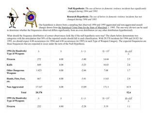
  • 1. Null Hypothesis: The use of knives in domestic violence incidents has significantly changed during 1994 and 1995. Research Hypothesis: The use of knives in domestic violence incidents has not changed during 1994 and 1995. Our hypothesis is drawn from a sampling that observed 1994 and 1995 aggravated and non-aggravated assault charges drawn from the Statistical Crime Data for the State of Maryland, c. 1995. The one-way chi-test can be used to determine whether the frequencies observed differs significantly from an even distribution (or any other distribution hypothesized). What should the frequency distribution of correct observances look like if the null hypothesis were true? The charts below demonstrate two categories with the anticipation that 50% of the reported results should fall in each classification. With 20.378 incidents for 1994 and 24.021 for 1995, we should expect 4.08 occurrences (in 1994) and 4.80 occurrences (in 1995) in each Type of Weapon Category. The expected frequencies are those frequencies that are expected to occur under the term of the Null Hypothesis. 1994 (In Hundreds) fo fe fo - fe (fo - fe)2 (fo - fe)2 Type of Weapons fe Firearm .272 4.08 -3.80 14.44 3.5 Knife .849 4.08 -3.23 10.43 2.6 Other Dangerous 1.423 4.08 -2.66 7.08 1.7 Weapons Hands, Fists, Feet, .667 4.08 -3.41 11.63 2.9 etc. Non-Aggravated 17.167 4.08 13.09 171.3 41.9 Total 20.378 52.6 1995 (In Hundreds) fo fe fo - fe (fo - fe)2 (fo - fe)2 Type of Weapons fe Firearm .252 4.80 -2.28 5.19 1.1
  • 2. Knife 1.074 4.80 -3.73 13.91 2.9 Other Dangerous 1.771 4.80 -3.03 9.18 1.9 Weapons Hands, Fists, Feet, .672 4.80 -4.13 17.06 3.6 etc. Non-Aggravated 20.252 4.80 15.45 238.70 49.7 Total 24.021 59.2 Null Hypothesis: The use of knives in domestic violence incidents has significantly changed during 1994 and 1995. Research Hypothesis: The use of knives in domestic violence incidents has not changed during 1994 and 1995. (Continued) The chi-squared method allows us to test the significance of the difference between a set of observed frequencies and expected frequencies. Based on just the observed and expected frequencies, the formula for chi-square is: (fo - fe)2 X2 = Σ fe where fo = observed frequency in any category fe = expected frequency in any category Our next step is to interpret the chi-square value by determining the appropriate degrees of freedom. df = k - 1 where k = number of categories in the observed frequency distribution. Our example shows 5 categories (firearms; knives; other dangerous weapons; hands, fists, feet, etc.; and non-aggravated) in 1994 and 1995:
  • 3. df = 5 - 1 = 4 Now by checking The Critical Value of Chi-Square at the .05 and .01 Chart, we look for the .05 significant level to check 4 degrees of freedom. The value is 9.488. This is the value that we must exceed before we can reject the null hypothesis. Because our calculated chi-square for 1994 is 52.6 and for 1995 is 59.2, it is larger than the table value, we reject the null hypothesis and accept the research hypothesis. The observed frequencies do differ significantly from the expected occurrence for an equal distribution under the null hypothesis for knife usage in domestic violence situations. In comparing the chi-squared test to our obtained frequencies, the reported sampling did not indicate a perfectly even distribution (4.08 in 1994 and 4.80 in 1995 for each type of weapon), the degree of unevenness was sufficiently large. Null Hypothesis: Unknown factors do not play a significant role in domestic violence occurrences during 1994 and 1995. Research Hypothesis: Unknown factors do play a significant role in domestic violence occurrences during 1994 and 1995. This hypothesis was also taken from a sampling that observed 1994 and 1995 unknown factors in domestic violence drawn from The Statistical Crime Data for the State of Maryland, c. 1995. Again, the one-way chi-test will be used to determine whether the frequencies observed differs significantly from an even distribution (or any other distribution hypothesized). We want to demonstrate if this frequency distribution for unknown factors shows if the null hypothesis is true? The charts below demonstrate two categories with the anticipation that 50% of the reported results should fall in each classification. With 20.378 incidents for 1994 and 24.021 incidents for 1995, we should expect .926 occurrences (in 1994) and 1.091 occurrences (in 1995) for each year’s Circumstances Category. The expected frequencies are those incidents that are expected to occur under the term of the Null Hypothesis. 1994 (In fo fe fo - fe (fo - fe)2 (fo - fe)2 Hundreds)
  • 4. Circumstances fe Alcohol 2.686 .926 1.76 3.098 3.4 Drugs .373 .926 -0.553 .306 .3 Food/Cooking .100 .926 -0.826 .682 .7 Friends .169 .926 -0.757 .573 .6 Gambling .005 .926 -0.921 .848 .9 Household .128 .926 -0.798 .637 .7 Chores Infidelity 1.055 .926 0.129 .017 0 Employment/Job .104 .926 -0.822 .676 .7 Mental .090 .926 -0.836 .699 .8 Imbalance Money .817 .926 -0.109 .012 0 Children .914 .926 -0.012 1.44 1.6 Property .609 .926 -0.317 .100 .1 Relative .114 .926 -0.812 .659 .7 Sex .168 .926 -0.758 .575 .6 Hobby .011 .926 -0.915 .837 .9 T.V. .054 .926 -0.872 .760 .8
  • 5. Separation .628 .926 -0.298 .089 .1 Divorce .129 .926 -0.797 .635 .7 Reconciliation .030 .926 -0.896 .803 .9 Out Late .398 .926 -0.528 .279 .3 Other 3.716 .926 2.79 7.784 8.4 Unknown 8.080 .926 7.154 51.180 55.3 Total 20.378 78.5 1995 (In fo fe fo - fe (fo - fe)2 (fo - fe)2 Hundreds) fe Circumstances Alcohol 3.139 1.091 2.048 4.194 3.8 Drugs .458 1.091 -.633 .401 .4 Food/Cooking .163 1.091 -.928 .861 .8 Friends .278 1.091 -.813 .661 .6 Gambling .012 1.091 -1.079 1.164 .1 Household .162 1.091 -.929 .863 .8 Chores Infidelity 1.372 1.091 .281 .079 .1 Employment/Job .122 1.091 -.969 .939 .9
  • 6. Mental .110 1.091 -.981 .962 .9 Imbalance Money 1.043 1.091 .048 2.304 2.1 Children 1.181 1.091 .09 8.1 7.4 Property .963 1.091 -.128 .016 .0 Relative .202 1.091 -.889 .790 1.4 Sex .224 1.091 -.867 .752 .7 Hobby .011 1.091 -1.08 1.166 .1 T.V. .061 1.091 -1.03 1.061 .9 Separation .901 1.091 .19 .036 .0 Divorce .162 1.091 .929 .863 .8 Reconciliation .037 1.091 1.054 1.111 1.0 Out Late .510 1.091 -.581 .338 .3 Other 2.877 1.091 1.786 3.190 2.9 Unknown 10.033 1.091 8.942 79.96 73.29 Total 24.021 101.29 Null Hypothesis: Unknown factors do not play a significant role in domestic violence occurrences during 1994 and 1995.
  • 7. Research Hypothesis: Unknown factors do play a significant role in domestic violence occurrences during 1994 and 1995. (Continued) The chi-squared method allows us to test the significance of the difference between a set of observed frequencies and expected frequencies. Based on just the observed and expected frequencies, the formula for chi-square is: (fo - fe)2 X2 = Σ fe where fo = observed frequency in any category fe = expected frequency in any category Our next step is to interpret the chi-square value by determining the appropriate degrees of freedom. df = k - 1 where k = number of categories in the observed frequency distribution. Our example shows 22 categories (Alcohol, Drugs, Food/Cooking, Friends, Gambling, Household Chores, Infidelity, Employment/Job, Mental Imbalance, Money, Children, Property, Relative, Sex, Hobby, T.V., Separation, Divorce, Reconciliation, Out Late, Other and Unknown) in 1994 and 1995: df = 22 - 1 = 21 Now by checking The Critical Value of Chi-Square at the .05 and .01 Chart, we look for the .05 significant level to check 21 degrees of freedom. The value is 32.671. This is the value that we must exceed before we can reject the null hypothesis. Because our calculated chi-square for 1994 is 78.5 and for 1995 is 101.29, it is larger than the table value, we reject the null hypothesis and accept the research hypothesis. The observed frequencies do differ significantly from the expected occurrence for an equal distribution under the null hypothesis for unknown factors in domestic violence situations. In comparing the chi-squared test to our obtained frequencies, the reported sampling did not indicate a perfectly even distribution (.926 in 1994 and 1.091 in 1995 for each circumstance), the degree of unevenness was sufficiently large.
  • 8. Null Hypothesis: The morning hours have an effect on domestic violence during 1994 and 1995. Research Hypothesis: The morning hours have no effect on domestic violence during 1994 and 1995. The above hypothesis was also taken from a sampling that observed domestic violence’s 1994 and 1995 incidents occurring in the morning hours. This sample was also drawn from The Statistical Crime Data for the State of Maryland, c. 1995. Again, the one-way chi-test will be used to determine whether the frequencies observed differs significantly from an even distribution (or any other distribution hypothesized). We want to demonstrate if this frequency distribution for the morning hours shows if the null hypothesis is true? The charts below demonstrate two categories with the anticipation that 50% of the reported results should fall in each classification. With 76.95 incidents for 1994 and 93.57 incidents for 1995, we should expect 6.41 morning occurrences (in 1994) and 7.80 morning occurrences (in 1995) for each year’s Morning Hours Category. The expected frequencies are those incidents that are expected to occur under the term of the Null Hypothesis. 1994 (In Hundreds) fo fe fo - fe (fo - fe)2 (fo - fe)2 Morning Hours fe 12:00 A.M. 9.85 6.41 3.44 11.83 1.8 1:00 A.M. 10.6 6.41 4.19 17.56 2.7 2:00 A.M. 8.34 6.41 1.93 3.72 .6 3:00 A.M. 6.38 6.41 -.03 9 1.4
  • 9. 4:00 A.M. 4.33 6.41 -2.08 4.33 .7 5:00 A.M. 2.92 6.41 -3.49 12.18 1.9 6:00 A.M. 3.22 6.41 -3.19 10.17 1.6 7:00 A.M. 3.29 6.41 -3.12 9.73 1.5 8:00 A.M. 4.58 6.41 -1.83 3.35 .5 9:00 A.M. 5.92 6.41 -.49 .24 .0 10:00 A.M. 7.91 6.41 1.5 2.25 .4 11:00 A.M. 9.61 6.41 3.2 10.24 1.6 Total 76.95 14.7 1995 (In Hundreds) fo fe fo - fe (fo - fe)2 (fo - fe)2 Morning Hours fe 12:00 A.M. 12.89 7.8 5.09 25.9 3.3 1:00 A.M. 13.17 7.8 5.37 28.8 3.7 2:00 A.M. 10.7 7.8 2.9 8.41 1.1 3:00 A.M. 8.02 7.8 .22 .04 5.1 4:00 A.M. 4.97 7.8 -2.83 8 1 5:00 A.M. 3.79 7.8 -4.01 16 2.1 6:00 A.M. 3.44 7.8 -4.36 19 2.4
  • 10. 7:00 A.M. 4.17 7.8 -3.63 13.2 1.7 8:00 A.M. 5.45 7.8 -2.35 5.52 .7 9:00 A.M. 7.22 7.8 -.58 .34 0 10:00 A.M. 9.34 7.8 1.54 2.37 .3 11:00 A.M. 10.41 7.8 2.61 6.81 .9 Total 93.57 22.3 Null Hypothesis: The morning hours have an effect on domestic violence occurrences during 1994 and 1995. Research Hypothesis: The morning hours have no effect on domestic violence occurrences during 1994 and 1995. (Continued) The chi-squared method allows us to test the significance of the difference between a set of observed frequencies and expected frequencies. Based on just the observed and expected frequencies, the formula for chi-square is: (fo - fe)2 X2 = Σ fe where fo = observed frequency in any category fe = expected frequency in any category Our next step is to interpret the chi-square value by determining the appropriate degrees of freedom.
  • 11. df = k - 1 where k = number of categories in the observed frequency distribution. Our example shows 12 categories (from 12:00 a.m. until 11:00 a.m.) in 1994 and 1995: df = 12 - 1 = 11 Now by checking The Critical Value of Chi-Square at the .05 and .01 Chart, we look for the .05 significant level to check 11 degrees of freedom. The value is 19.675. This is the value that we must exceed before we can reject the null hypothesis. Because our calculated chi-square for 1994 is 14.7 and for 1995 is 22.3, it is smaller than the table value, we accept the null hypothesis and reject the research hypothesis. The observed frequencies do not differ significantly from the expected occurrence for an equal distribution under the null hypothesis for morning incidents in domestic violence situations. In comparing the chi-squared test to our obtained frequencies, the reported sampling did indicate a perfectly even distribution (6.41 in 1994 and 7.8 in 1995 for each circumstance) for the Morning Hours Category in 1994. However, comparing the chi-squared test to our obtained frequencies for the Morning Hours Category in 1995, the reported sampling did not indicate a perfectly even distribution (6.41 in 1994 and 7.8 in 1995 for each circumstance) the degree of unevenness was significantly large. Null Hypothesis: The afternoon hours have an effect on domestic violence occurrences during 1994 and 1995. Research Hypothesis: The afternoon hours have no affect on domestic violence occurrences during 1994 and 1995. The above hypothesis was also taken from a sampling that observed domestic violence 1994 and 1995 incidents occurring in the afternoon hours. This sample was also drawn from The Statistical Crime Data for the State of Maryland, c. 1995. Again, the one-way chi-test will be used to determine whether the frequencies observed differs significantly from an even distribution (or any other distribution hypothesized). We want to demonstrate if this frequency distribution for the afternoon hours shows if the null hypothesis is true? The charts below demonstrate two categories with the anticipation that 50% of the reported results should fall in each classification. With 76.95 incidents for 1994 and 93.57
  • 12. incidents for 1995, we should expect 5 morning occurrences (in 1994) and 6 morning occurrences (in 1995) for each year’s Afternoon Hours Category. The expected frequencies are those incidents that are expected to occur under the term of the Null Hypothesis. 1994 (In Hundreds) fo fe fo - fe (fo - fe)2 (fo - fe)2 Afternoon Hours fe 12:00 P.M. 8.17 10.57 -2.4 5.76 .5 1:00 P.M. 6.79 10.57 -3.78 14.29 1.4 2:00 P.M. 9.43 10.57 -1.14 1.3 .1 3:00 P.M. 9.89 10.57 -.068 .46 0 4:00 P.M. 9.99 10.57 -.58 .34 0 5:00 P.M. 8.87 10.57 -1.7 2.89 .3 6:00 P.M. 10 10.57 -.57 .32 0 7:00 P.M. 11.58 10.57 1.01 1.02 .1 8:00 P.M. 11.93 10.57 1.36 1.85 .2 9:00 P.M. 12.57 10.57 2 4 .4 10:00 P.M. 13.98 10.57 3.41 11.63 1.1 11:00 P.M. 13.63 10.57 3.06 9.36 .9 Total 76.95 5 1995 (In Hundreds) fo fe fo - fe (fo - fe)2 (fo - fe)2
  • 13. Afternoon Hours fe 12:00 P.M. 10.42 12.22 -1.8 25.9 .3 1:00 P.M. 8.09 12.22 -4.13 28.8 1.4 2:00 P.M. 10.05 12.22 -2.17 8.41 .4 3:00 P.M. 10.66 12.22 -1.56 .04 .2 4:00 P.M. 10.43 12.22 -1.79 8 .3 5:00 P.M. 10.05 12.22 -2.17 16 .4 6:00 P.M. 11.61 12.22 -.61 19 0 7:00 P.M. 13.21 12.22 .99 13.2 0 8:00 P.M. 14.34 12.22 2.12 5.52 .4 9:00 P.M. 15.23 12.22 3.01 .34 .7 10:00 P.M. 16.08 12.22 3.86 2.37 1.2 11:00 P.M. 16.47 12.22 4.25 6.81 .7 Total 146.64 6 Null Hypothesis: The afternoon hours have an effect on domestic violence occurrences during 1994 and 1995. Research Hypothesis: The afternoon hours have no effect on domestic violence occurrences during 1994 and 1995.
  • 14. (Continued) The chi-squared method allows us to test the significance of the difference between a set of observed frequencies and expected frequencies. Based on just the observed and expected frequencies, the formula for chi-square is: (fo - fe)2 X2 = Σ fe where fo = observed frequency in any category fe = expected frequency in any category Our next step is to interpret the chi-square value by determining the appropriate degrees of freedom. df = k - 1 where k = number of categories in the observed frequency distribution. Our example shows 12 categories (from 12:00 p.m. through 11:00 p.m.) in 1994 and 1995: df = 12 - 1 = 11 Now by checking The Critical Value of Chi-Square at the .05 and .01 Chart, we look for the .05 significant level to check 11 degrees of freedom. The value is 19.675. This is the value that we must exceed before we can reject the null hypothesis. Because our calculated chi-square for 1994 is 5 and for 1995 is 6, it is smaller than the table value, we accept the null hypothesis and reject the research hypothesis. The observed frequencies do not differ significantly from the expected occurrence for an equal distribution under the null hypothesis for morning incidents in domestic violence situations. In comparing the chi-squared test to our obtained frequencies, the reported sampling did indicate a perfectly even distribution (10.57 in 1994 and 12.22 in 1995 for each circumstance). Null Hypothesis: The months of the year have an effect on domestic violence during 1994 and 1995.
  • 15. Research Hypothesis: The months of the year have no affect on domestic violence during 1994 and 1995. The above hypothesis was also taken from a sampling that observed domestic violence 1994 and 1995 incidents occurring in the month of the year. This sample was also drawn from The Statistical Crime Data for the State of Maryland, c. 1995. Again, the one-way chi-test will be used to determine whether the frequencies observed differs significantly from an even distribution (or any other distribution hypothesized). We want to demonstrate if this frequency distribution for the month of the year shows if the null hypothesis is true? The charts below demonstrate two categories with the anticipation that 50% of the reported results should fall in each classification. With 20.378 incidents for 1994 and 24.021 incidents for 1995, we should expect 1.7 monthly occurrences (in 1994) and 2 monthly occurrences (in 1995) for each of the year’s Month of the Year Category. The expected frequencies are those incidents that are expected to occur under the term of the Null Hypothesis. 1994 (In Hundreds) fo fe fo - fe (fo - fe)2 (fo - fe)2 Month of Year fe January 1.542 1.7 -.158 .03 .014 February 1.486 1.7 -.214 .05 .027 March 1.734 1.7 .034 .001 0 April 1.710 1.7 .01 0 0 May 1.690 1.7 -.01 0 0
  • 16. June 1.705 1.7 .005 0 0 July 1.822 1.7 .122 .01 0 August 1.812 1.7 .112 .01 0 September 1.834 1.7 .134 .02 0 October 1.804 1.7 .104 .01 0 November 1.666 1.7 .034 .001 0 December 1.573 1.7 .127 .02 0 Total 20.378 .041 1995 (In Hundreds) fo fe fo - fe (fo - fe)2 (fo - fe)2 Month of Year fe January 1.937 2 -.063 .001 .005 February 1.526 2 -.474 .224 .112 March 1.941 2 -.059 .002 .001 April 1.906 2 -.094 .001 .005 May 2.128 2 .128 .02 .01 June 2.046 2 .046 2.12 1.06 July 2.277 2 .277 .08 .139 August 2.181 2 .181 .03 .015
  • 17. September 2.003 2 .003 0 0 October 1.986 2 -.014 0 0 November 1.918 2 -.082 .006 .003 December 2.172 2 .172 .029 .015 Total 24.021 1.365 Null Hypothesis: The months of the year have an effect on domestic violence during 1994 and 1995. Research Hypothesis: The months of the year have no effect on domestic violence during 1994 and 1995. (Continued) The chi-squared method allows us to test the significance of the difference between a set of observed frequencies and expected frequencies. Based on just the observed and expected frequencies, the formula for chi-square is: (fo - fe)2 X2 = Σ fe where fo = observed frequency in any category fe = expected frequency in any category Our next step is to interpret the chi-square value by determining the appropriate degrees of freedom. df = k - 1 where k = number of categories in the observed frequency distribution. Our example shows 12 categories (from January through December) in 1994 and 1995:
  • 18. df = 12 - 1 = 11 Now by checking The Critical Value of Chi-Square at the .05 and .01 Chart, we look for the .05 significant level to check 11 degrees of freedom. The value is 19.675. This is the value that we must exceed before we can reject the null hypothesis. Because our calculated chi-square for 1994 is .041 and for 1995 is 1.365, it is smaller than the table value, we accept the null hypothesis and reject the research hypothesis. The observed frequencies do not differ significantly from the expected occurrence for an equal distribution under the null hypothesis for monthly incidents in domestic violence situations. In comparing the chi-squared test to our obtained frequencies, the reported sampling did indicate a perfectly even distribution (1.7 in 1994 and 2 in 1995 for each circumstance). Null Hypothesis: The day of the week has an affect on domestic violence occurring in 1994 and 1995. Research Hypothesis: The day of the week has no effect on domestic violence occurring in 1994 and 1995. The above hypothesis was also taken from a sampling that observed domestic violence 1994 and 1995 incidents occurring on a certain day of the week. This sample was also drawn from The Statistical Crime Data for the State of Maryland, c. 1995. Again, the one-way chi-test will be used to determine whether the frequencies observed differs significantly from an even distribution (or any other distribution hypothesized). We want to demonstrate if this frequency distribution for the day of the week shows if the null hypothesis is true? The charts below demonstrate two categories with the anticipation that 50% of the reported results should fall in each classification. With 20.378 incidents for 1994 and 24.021 incidents for 1995, we should expect 2.911 monthly occurrences (in 1994) and 3.432 monthly occurrences (in 1995) for each of the year’s Day of the Week Category. The expected frequencies are those incidents that are expected to occur under the term of the Null Hypothesis.
  • 19. 1994 (In Hundreds) fo fe fo - fe (fo - fe)2 (fo - fe)2 Day of Week fe Monday 3.017 2.911 .106 .011 .003 Tuesday 2.703 2.911 -.208 .043 .015 Wednesday 2.457 2.911 -.454 .206 .07 Thursday 2.479 2.911 -.432 .187 ..064 Friday 2.846 2.911 -.065 .004 .001 Saturday 3.290 2.911 .379 .144 .049 Sunday 3.586 2.911 .675 .456 .157 Total 20.378 .359 1995 (In Hundreds) fo fe fo - fe (fo - fe)2 (fo - fe)2 Day of Week fe Monday 3.322 3.432 -.11 .012 3.5 Tuesday 3.246 3.432 -.186 .346 .01 Wednesday 3.019 3.432 -.413 .171 .05 Thursday 2.956 3.432 -.476 .227 .07 Friday 3.207 3.432 -.225 .051 .01 Saturday 3.980 3.432 .548 .3 .08
  • 20. Sunday 4.291 3.432 .859 .738 .02 Total 24.021 3.74 Null Hypothesis: The day of the week has an effect on domestic violence occurring in 1994 and 1995. Research Hypothesis: The day of the week has no effect on domestic violence occurring in 1994 and 1995. (Continued) The chi-squared method allows us to test the significance of the difference between a set of observed frequencies and expected frequencies. Based on just the observed and expected frequencies, the formula for chi-square is: (fo - fe)2 X2 = Σ fe where fo = observed frequency in any category fe = expected frequency in any category Our next step is to interpret the chi-square value by determining the appropriate degrees of freedom. df = k - 1 where k = number of categories in the observed frequency distribution. Our example shows 7 categories (from Monday through Sunday) in 1994 and 1995: df = 7 - 1 = 6 Now by checking The Critical Value of Chi-Square at the .05 and .01 Chart, we look for the .05 significant level to check 6 degrees of freedom. The value is 12.592. This is the value that we must exceed before we can reject the null hypothesis. Because our calculated chi-square for 1994 is .359 and for 1995 is 3.74, it is smaller than the table value, we accept the null hypothesis and reject the research hypothesis. The observed frequencies do
  • 21. not differ significantly from the expected occurrence for an equal distribution under the null hypothesis for day of the week incidents in domestic violence situations. In comparing the chi-squared test to our obtained frequencies, the reported sampling did indicate a perfectly even distribution (2.911 in 1994 and 3.432 in 1995 for each circumstance). INTRODUCTION The act of domestic violence has no label. It could happen to any gender, at any age and in any occupation. Domestic violence can also take on the form of mental, physical, verbal, emotional, and psychological abuse. The ultimate goal of a domestic violence abuser is to have total control and power over another person. This situation can be inflicted upon anyone at anytime. Russell Hovan’s perspective states, “There are situations in life to which the only satisfactory response is a physically violent one. If you don’t make that response, you continually relive the unresolved situation over and over in your life.” (b. 1925, U.S. author. Novelists in Interview (ed. by John Haffenden, 1985)). The scariest account of domestic violence occurs when you do not have to see a scar to feel one. It’s like a thief in the night, because we don’t think about it until it indirectly or directly affects us on a personal level. There are many cases that have unknown causes and probably as many that go unreported. It’s a time bomb waiting to explode, and we will show the impact of the explosion by reviewing 1994 and 1995 domestic violence data. Our source was provided through the publication, The Statistical Crime Data for the State of Maryland. By using the chi-squared test, it will demonstrate if there is a significant or insignificant trend. CONCLUSION
  • 22. As the data shows, domestic violence in the State of Maryland for 1994 and 1995 indicates it is on the rise. We must all take steps to neutralize this time bomb. Because everybody is a victim as long as the abuse continues. In addition, everyone must begin to take an active and responsible role to curve this silent offense. As long as we continue to allow these abuses to perpetuate, we are threatening our own futures. If the trend continues to rise as it has been reported in 1994 and 1995, our children’s behaviors may grow more vicious in nature.