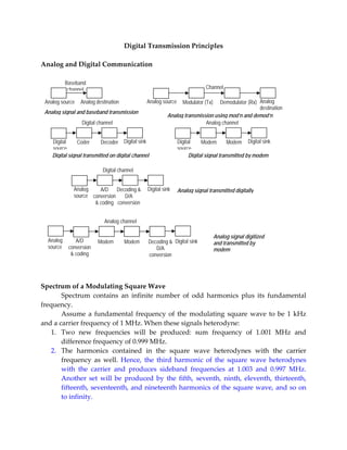
1. Digital Transmission Principles
Analog and Digital Communication
Baseband
channel Channel
Analog source Analog destination Analog source Modulator (Tx)Demodulator (Rx) Analog
destination
Analog signal and baseband transmission
Analog transmission using mod’n and demod’n
Digital channel Analog channel
Digital Coder Decoder Digital sink Digital Modem Modem Digital sink
source source
Digital signal transmitted on digital channel Digital signal transmitted by modem
Digital channel
Analog A/D Decoding & Digital sink Analog signal transmitted digitally
source conversion D/A
& coding conversion
Analog channel
Analog signal digitized
Analog A/D Modem Modem Decoding & Digital sink and transmitted by
source conversion D/A modem
& coding conversion
Spectrum of a Modulating Square Wave
Spectrum contains an infinite number of odd harmonics plus its fundamental
frequency.
Assume a fundamental frequency of the modulating square wave to be 1 kHz
and a carrier frequency of 1 MHz. When these signals heterodyne:
1. Two new frequencies will be produced: sum frequency of 1.001 MHz and
difference frequency of 0.999 MHz.
2. The harmonics contained in the square wave heterodynes with the carrier
frequency as well. Hence, the third harmonic of the square wave heterodynes
with the carrier and produces sideband frequencies at 1.003 and 0.997 MHz.
Another set will be produced by the fifth, seventh, ninth, eleventh, thirteenth,
fifteenth, seventeenth, and nineteenth harmonics of the square wave, and so on
to infinity.

2. Spectrum distribution when modulating with a square wave.
The first set of sidebands is directly related to the amplitude of the square wave.
The second set of sidebands is related to the third harmonic content of the square wave
and is 1/3 the amplitude of the first set. The third set is related to the amplitude of the
first set of sidebands and is 1/5 the amplitude of the first set. This relationship will
apply to each additional set of sidebands.
Various square‐wave modulation levels with frequency‐spectrum carrier and
sidebands.
Observations: (carrier modulated with a square wave)
1. As the amplitude of the modulating square wave is increased, the RF peaks
increases in amplitude during the positive alternation of the square wave and
decrease during the negative half of the square wave.
2. For the frequency spectrum, the carrier amplitude remains constant, but the
sidebands increase in amplitude in accordance with the amplitude of the
modulating square wave.
3. In view (C) the amplitude of the square wave of voltage is equal to the peak
voltage of the unmodulated carrier wave. This is 100% modulation, just as in
conventional AM.
4. In the frequency spectrum, the sideband distribution is also the same as in AM.
The total sideband power is 1/2 of the total power when the modulator signal is a
square wave. This is in contrast to 1/3 of the total power with sine‐wave
modulation.
5. In view (D), the increase of the square‐wave modulating voltage is greater in
amplitude than the unmodulated carrier. The sideband distribution does not

3. change; but, as the sidebands take on more of the transmitted power, so will the
carrier.
In pulse modulation, the same general rules apply as in AM.
Pulse Timing
Some pulse‐modulation systems modulate a carrier in the manner of increasing
or decreasing the amplitude of the modulating square wave. Others produce no RF
until pulsed; that is, RF occurs only during the actual pulse. If we allow oscillations to

4. occur for a given period of time only during selected intervals, as in view (B), we are
PULSING the system.
Pulse Transmission
Note: The pulse transmitter is gated on and off instead of being modulated by a square
wave.
Varying pulse‐modulating waves
Note: Carrier frequencies in pulse systems can vary.
The carrier frequency is not the only frequency we must concern ourselves with
in pulse systems. We must also note the frequency that is associated with the repetition
rate of groups of pulses.
Pulse‐repetition time (PRT) ‐ the total time of one complete pulse cycle of operation
(rest time plus pulse width)
Pulse‐repetition frequency (PRF) — the rate, in pulses per second, that the pulse occurs

5. Pulse‐repetition time (prt) and pulse‐repetition frequency (prf)
Figure 2-34.—Pulse cycles.
Pulse width — the duration of time RF frequency is transmitted
Rest time — the time the transmitter is resting (not transmitting)
.
Pulse width and rest time
The pulse width is the time that the transmitter produces RF oscillations and is
the actual pulse transmission time. During the nonpulse time, the transmitter produces
no oscillations and the oscillator is cut off.
Power in a Pulse System
Peak power ‐ the maximum value of the transmitted pulse
Average power ‐ peak power value averaged over the pulse‐repetition time.
Peak power is very easy to see in a pulse system.

6. Duty Cycle ‐ ratio of actual transmitting time to transmitting time plus rest time. To
establish the duty cycle, divide the pulse width by the pulse repetition time of the
system.
Digital transmission – transmission of digital signals between two or more points in a
communication system
Advantages of Digital Transmission
1. Noise immunity, since it is not necessary to evaluate the precise amplitude,
frequency or phase to ascertain logic condition. A simple determination is made
whether the pulse is above or below a prescribed level.
2. Digital signals are better suited than analog signals for processing and
multiplexing. It is easier to store digital signals and the transmission rate can be
varied to adapt different environments and to interface with different types of
equipment.
3. More resistant to analog systems to additive noise because they use signal
regeneration rather than signal amplification.
4. Simpler to measure and evaluate than analog signals
Advantages of Digital Transmission
1. Transmission of digitally encoded analog signals requires significantly more
bandwidth than simply transmitting the original analog signal.
2. Analog signals must be converted to digital pulses prior to transmission and
converted back to analog form at the receiver, thus requiring additional encoding
and decoding circuitry
3. Requires precise time synchronization between the clocks in the transmitters and
receivers
4. Some digital transmission systems are incompatible with older analog
transmission systems.
Communications Pulse Modulators
To transmit intelligence using pulse modulation, one must provide a method to
vary some characteristic of the pulse train in accordance with the modulating signal.
The characteristics of these pulses that can be varied are amplitude, pulse width, pulse‐
repetition time, and the pulse position as compared to a reference. In addition to these
three characteristics, pulses may be transmitted according to a code to represent the
different levels of the modulating signal.
Pulse‐Amplitude Modulation

7. Pulse‐amplitude modulation (PAM) in which the amplitude of each pulse is
controlled by the instantaneous amplitude of the modulating signal at the time of each
pulse.
• The simplest form of pulse modulation.
• Generated in much the same manner as analog‐amplitude modulation.
• The timing pulses are applied to a pulse amplifier in which the gain is controlled
by the modulating waveform.
• Since these variations in amplitude actually represent the signal, this type of
modulation is basically a form of AM. The only difference is that the signal is
now in the form of pulses.
• Have the same built‐in weaknesses as any other AM signal ‐ high susceptibility
to noise and interference.
• The reason for susceptibility to noise is that any interference in the transmission
path will either add to or subtract from any voltage already in the circuit (signal
voltage). Thus, the amplitude of the signal will be changed. Since the amplitude
of the voltage represents the signal, any unwanted change to the signal is
considered a SIGNAL DISTORTION. For this reason, PAM is not often used.
When PAM is used, the pulse train is used to frequency modulate a carrier for
transmission.
Demodulating PAM: Peak detection uses the amplitude of a PAM signal or the duration
of a PWM signal to charge a holding capacitor and restore the original waveform. This
demodulated waveform will contain some distortion because the output wave is not a
pure sine wave. However, this distortion is not serious enough to prevent the use of
peak detection.

8. Pulse‐Time Modulation
Time characteristics of pulses may also be modulated with intelligence
information. Two time characteristics may be affected:
1. the time duration of the pulses, referred to as pulse‐duration modulation
(PDM) or pulse‐width modulation (PWM)
2. the time of occurrence of the pulses, referred to as pulse‐position
modulation (PPM)
A special type of pulse‐time modulation (PTM) referred to as pulse‐frequency
modulation (PFM) may also be employed.
Pulse‐time modulation (PTM) ‐ PDM.

9. Pulse‐time modulation (PTM) ‐ PPM
Pulse‐time modulation (PTM) ‐ PPM
Pulse‐duration modulation (pulse‐width modulation)
• The width of each pulse in a train is made proportional to the instantaneous
value of the modulating signal at the instant of the pulse. Either the leading
edges, the trailing edges, or both edges of the pulses may be modulated to
produce the variation in pulse width.
• PWM is often used because it is of a constant amplitude and is, therefore, less
susceptible to noise.
Generating PWM: Add the modulating signal to a repetitive sawtooth waveform. The
resulting waveform is then applied to a one‐shot multivibrator circuit which changes
state when the input signal exceeds a specific threshold level. The action produces
pulses with widths that are determined by the length of time that the input waveform
exceeds the threshold level.
Demodulating PWM: The peak detector circuit may also be used for PWM. To detect
PWM, modify the peak detector so that the time constant for charging C1 through CR1
is at least 10 times the maximum received pulse width. This may be done by adding a
resistor in series with the cathode or anode circuit of CR1. The amplitude of the voltage
to which C1 charges, before being discharged by the negative pulse, will be directly
proportional to the input pulse width. A longer pulse width allows C1 to charge to a
higher potential than a short pulse. This charge is held, because of the long time
constant of R1 and C1, until the discharge pulse is applied to diodes CR2 and CR3 just
prior to the next incoming pulse. These charges across C1 result in a wave shape similar
to the output shown for PAM detection.
Comparing PWM with PPM

10. Disadvantage: Varying pulse, width and therefore, of varying power content. This
means that the transmitter must be powerful enough to handle the maximum‐width
pulses, although the average power transmitted is much less than peak power.
Advantage: PWM will still work if the synchronization between the transmitter and
receiver fails; in PPM it will not,
Pulse‐position modulation
— The amplitude and width of the pulse is kept constant in the system. The position of
each pulse, in relation to the position of a recurrent reference pulse, is varied by each
instantaneous sampled value of the modulating wave.
Generating PPM: Apply PWM pulses to a differentiating circuit. This provides positive‐
and negative‐polarity pulses that correspond to the leading and trailing edges of the
PWM pulses. The position of the leading edge is fixed, whereas the trailing edge is not.
After differentiation, the negative pulses are position‐modulated in accordance with the
modulating waveform. Both the negative and positive pulses are then applied to a
rectification circuit. This application eliminates the positive, non‐modulated pulses and
develops a PPM pulse train
Demodulating PPM: PPM, PFM and PCM are most easily demodulated by first
converting them to either PWM or PAM. The trigger pulses must be synchronized with
the unmodulated position of the PPM pulses, but with a fixed time delay from these
pulses. As the position‐modulated pulse is applied to the flip‐flop, the output is driven
positive. After a period of time, the trigger pulse is again generated and drives the flip‐
flop output negative and the pulse ends. Because the PPM pulses are constantly varying
in position with reference to the unmodulated pulses, the output of the flip‐ flop also
varies in duration or width. This PWM signal can now be applied to either a peak
detector or low‐pas filter for demodulation.
Comparing PPM with PWM
Advantage: requires constant transmitter power since the pulses are of constant
amplitude and duration
Disadvantage: depends on transmitter‐receiver synchronization
Pulse‐frequency modulation (PFM)
• PFM is a method of pulse modulation in which the modulating wave is
used to frequency modulate a pulse‐generating circuit. For example, the
pulse rate may be 8,000 pulses per second (pps) when the signal voltage is
0. The pulse rate may step up to 9,000 pps for maximum positive signal
voltage, and down to 7,000 pps for maximum negative signal voltage.

11. • This method of modulation is not used extensively because of complicated
PFM generation methods. It requires a stable oscillator that is frequency
modulated to drive a pulse generator. Since the other forms of PTM are
easier to achieve, they are commonly used.
Pulse‐Code Modulation
• Invented by Alec Reeves in 1937
• Most commonly used digital communications technique
• Form of pulse modulation where samples of the analog input are
converted to binary coded pulses
Block Diagram of a PCM Transmission System
Bandpass filter – limits the frequency of the analog signal to the voice band frequency
range
Sample‐and‐hold circuit – periodically samples the analog input signal and converts the
samples to multilevel PAM signal
ADC – converts the PAM samples to parallel PCM codes
Parallel‐to‐serial converter – converts the parallel PCM codes to serial digital pulses

12. Forms of Sampling
Natural sampling – tops of the sample pulses retain their original shape during the
sample interval
Flat‐top sampling – sampling of an analog signal using a sample‐and‐hold circuit, such
that the sample has the same amplitude for its whole duration
The sampling process alters the frequency spectrum and introduces aperture
error, which is when the amplitude of the sampled signal changes during the sample
time.
Sampling Theorem
For an analog receiver to be fully reconstructed at the receiver’s output, the rate
at which an analog input signal should be sampled must at least be twice the highest
audio frequency component present.
fs ≥ 2fa
Aliasing or foldover distortion – results when the signal is undersampled; distortion
created by using too low a sampling rate when coding an analog signal for digital
transmission
falias = fs – fa
Quantization – process of converting samples of the analog input as a number of
discrete values.
Quantization interval or quantum – magnitude difference between adjacent steps

13. Overload distortion or peak limiting – occurs if the magnitude of the sample exceeds
the highest quantization interval
Resolution – magnitude of a quantum; also equal to the voltage of the minimum step
size
Quantization range – (+) or (‐) one‐half the resolution
Quantization noise or quantization error – results when the sampled analog signal is
rounded off to the closest available code.
Max Qe = ½ Resolution
Dynamic Range – ratio of the largest possible magnitude to the smallest possible
magnitude that can de decoded by the DAC at the receiver.
V V
DR = max = max = 2 n − 1
Vmin Resn
Expressing DR in dB:
Vmax V
DR (dB) = 20 log = 20 log max = 20 log ( 2 n − 1) ≈ 6.02n
Vmin Resn
Coding Efficiency – a numerical indication of how efficiently a PCM code is utilized.
min. no. of bits (inc. sign bit)
Coding Eff = * 100
actual no. of bits (inc. sign bit)
Signal‐to‐Quantization Noise Ratio for Linear PCM codes (or SNR)
v2 / R
SQR (dB) = 10 log 2
(q / 12) / R
where: R = resistance (ohms) v2/R = ave. signal power (watts)
v = rms signal voltage (volts) (q2/12)/R = ave. quant. noise power (watts)
q = quantization interval (volts)
v2 v
Assuming equal resistances: SQR (dB) = 10 log 2 = 10.8 + 20 log
(q / 12) q
Alternatively:
SNRpk = 3M2 M = number of symbols or levels
Noting that M = 2 n (n = number of bits), SNRpk in dB is also:
SNRpk (dB) = 4.77 + 6.02n
If the ratio of the peak to mean signal power v2peak/v2ave be denoted by α, then the
average SNR is
SNR = 3 (22n) (1/ α)

14. Expressing in dB:
SNR (dB) = 4.77 + 6.02n – αdB
Note: For sinusoidal signals, α = 2 (or 3 dB), for Gaussian random signals, α = 16
(or 12 dB), and for speech, α = 16 (or 12 dB)
PCM Bit Rate = nfs
Note: CD systems use a standard sampling rate of 44.1 KHz.
Idle channel noise – random thermal noise quantized by the ADC when inputted at the
PCM sampler.
Nonlinear PCM
With voice transmission, low‐amplitude signals are more likely to occur than
large‐amplitude signals. As a result, there would be fewer codes available for higher
amplitudes, thereby increasing quantization error for larger‐amplitude signals. This
technique is called nonlinear encoding.
Companding Techniques (compressing then expanding)
With companded systems, higher‐amplitude signals are compressed (amplified
less than the lower‐amplitude signals prior to transmission) and then expanded
(amplified more than lower‐amplitude signals) in the receiver.
Analog Companding
I. μ‐law companding – North American standard for voice compression
V
ln (1 + μ in )
Vmax
Vout = Vmax
ln (1 + μ)
where: Vmax = max. uncompressed analog input amplitude (V)
Vin = amplitude of the input signal at a particular instant of time (V)
μ = parameter used to define the amount of compression
Vout = compressed output amplitude
Indicators: The higher the μ value, the higher the compression. For μ = 0, the curve is
linear (no compression). Most recent PCM systems use an 8‐bit code with μ = 255.
II. A‐law companding
AVin /Vmax V 1
Vout = Vmax 0 ≤ in ≤
1 + ln A Vmax A
1 + ln (AVin /Vmax ) 1 Vin
= ≤ ≤ 1
1 + ln A A Vmax

15. ITU Recommendation G.711 – recognizes A‐law and μ‐law as the international toll
quality standard for digital coding of voice frequency signals; uses a sampling rate of 8
kHz and 8 encoding law of 8 binary digits per sample.
Bandwidth Reduction Techniques
1. Differential Pulse Code Modulation ‐ the difference in the amplitude between
two successive samples is transmitted rather than the actual samples. The
adjacent samples derived from most naturally generated information signals are
not usually independent but correlated.
2. Adaptive Differential Pulse Code Modulation – a more sophisticated version of
DPCM; adopted by the ITU as the reduced bit rate standard. The ADPCM
encoder takes a 64‐kbps companded PCM signal (G.711) and converts it to a 32‐
kbps ADPCM signal (G.721). Other specifications are defined by the ITU‐T,
G.726 and G.727 for ADPCM with transmission rates of 16 kbps to 40 kbps.
3. Delta Modulation – uses a single‐bit PCM code to achieve digital transmission of
analog signals. (Algorithm: If the current sample is smaller than the previous
sample, a logic 0 is transmitted. If the current sample is larger than the previous
sample, a logic 1 is transmitted)
Problems Encountered on Delta Modulation
• Slope overload – The slope of the analog signal is greater than what the
delta modulator can maintain. To reduce slope overload, increase the
magnitude of the minimum step size.
• Granular noise – The reconstructed signal has variations that were not
present in the original signal. It can be reduced by decreasing the step
size.
4. Adaptive Delta Modulation – In conventional DM, the problem of keeping both
quantization noise and slope overload acceptably low is solved by oversampling
(keeping the DM size and sampling many times the Nyquist rate). The penalty
incurred is loss of some bandwidth savings, which is expected of DM. An
alternative strategy is to make the DM size variable, making it larger during
periods when slope overload would otherwise dominate and smaller when
granular noise might dominate. Such systems are called adaptive DM systems.
Digital companding
The analog signal is first sampled and converted to linear PCM code, after which
the code will be digitally compressed. In the receiver, the compressed PCM code is
expanded, then decoded (back to analog). Most recent PCM systems use a 12‐bit linear
PCM code and an 8‐bit compressed PCM code.
Problems:

16. 1. For a sample rate of 20 kHz, determine the maximum analog input frequency.
2. Determine the alias frequency for a 14‐kHz sample rate and an analog input
frequency of 8 kHz.
3. Find the Nyquist interval for a signal defined as 5 cos1000πt cos 4000πt
4. Determine the dynamic range for a 12‐bit sign‐magnitude PCM code
5. Determine the minimum number of bits required in a PCM code for a dynamic
range of 80 dB. What is the coding efficiency?
6. For a resolution of 0.04 V, determine the voltages for the following linear seven‐
bit magnitude PCM codes: (a) 0110101; (b) 1000001
7. Determine the range of an 8‐bit sign magnitude PCM code given as 10111000 if
its resolution is 0.1 V.
8. Determine the resolution and quantization error for an 8‐bit linear sign‐
magnitude PCM code for a maximum decoded voltage of 1.27 V.
9. Determine the SQR for a 2‐Vrms signal and a quantization interval of 0.2 V.
10. A digital communications system is to carry a single voice signal using linearly
quantized PCM. What bit rate will be required if an ideal anti‐aliasing filter with
a cut‐off frequency of 3.4 kHz is used at the transmitter at the SNR is to be kept
above 50 dB?
11. Given μ = 255, Vmax = 1 V and Vin = 0.75 V, determine the compressor gain.
12. A 12‐bit linear sign‐magnitude PCM code is digitally compressed into 8 bits. For
a resolution of 0.016 V, determine the following quantities for an input voltage of
‐6.592V (a) 12‐bit linear PCM code; (b) 8‐bit compressed PCM code; (c) decoded
12‐bit code; (d) decoded voltage; (e) percentage error
Motion Pictures Experts Group (MPEG) Compression Standards
MPEG‐1 – a lossy compression system, which is capable of achieving transparent,
perceptually lossless compression of stereophonic audio signals at high sampling rates.
Subjective listening tests performed by the MPEG Audio Committee, under very
difficult listening conditions, have shown that even with a 6‐to‐1 compression ratio, the
coded and original audio signals are perceptually identical. The MPEG‐1 coding
standard exploits two psychoacoustic characteristic of the auditory systems:
Critical Bands
Human ear – responds to incoming acoustical waves. It has three main parts:
Outer ear – aids in sound collection
Middle ear – provides an acoustical impedance match between the air and the cochlea
fluids, thereby conveying the vibrations of the tympanic membrane (eardrum) due to
incoming sounds to the inner ear in an efficient manner
Inner ear – converts the mechanical vibrations from the middle ear to an
electrochemical or neural signal for transmission to the brain for processing

17. The inner ear represents the power spectra of incoming signals on a nonlinear
scale in the form of limited frequency bands called the critical bands. The audible
frequency band, extending up to 20 kHz, is covered by 25 critical bands, whose
individual bandwidths increase with frequency. The auditory system may be viewed as
a band‐pass filter bank, consisting of 25 overlapping band‐pass filters with bandwidths
less than 100 Hz for the lowest audible frequencies and up to 5 kHz for the highest
audible frequencies.
Auditory Masking (noise masking) – frequency‐domain phenomenon that arises when
a low‐level signal (the maskee) and a high‐level signal (masker) occur simultaneously
and are close enough to each other in frequency. If the low‐level signal lies below a
masking threshold, it is made inaudible (masked) by the stronger signal. The auditory
masking is most pronounced when both signals lie in the same critical band, and less
effective when they lie in neighboring bands.
MPEG Audio Coding System
Transmitter
Digital (PCM) Encoded bit stream
audio signal Time-to-
frequency Quantizer Frame-packing
mapping and coder unit
network
Psychoacoustic
model
Encoded bit stream Digital (PCM)
Freq-sample Frequency-to- audio signal
Frame reconstruction time mapping
Unpacking unit network network
Receiver

18. Encoder Functions
Time‐to‐frequency mapping network – decompose the audio input signal into multiple
subbands for coding
The mapping is performed in three layers, labeled I, II and III, which are of
increasing complexity, delay and subjective perceptual performance.
Algorithm in Layer I – uses a band‐pass filter bank that divides the audio signal into 32
constant‐width subbands; this filter bank is also found in layers II and III. The design of
this filter bank is a compromise between computational efficiency and perceptual
performance.
Algorithm in Layer II – a simple enhancement of Layer I; it improves the compression
performance by coding the data in larger groups.
Algorithm in Layer III – much more refined and is designed to achieve frequency
resolutions closer to the partitions between the critical bands.
Psychoacoustic model – analyzes the spectral content of the audio input signal and
computes the signal‐to‐mask ratio for each subband in each of the three layers.
The information is, in turn, used by the quantizer‐coder to decide how to
apportion the available number of bits for the quantization of the subband signals. This
dynamic allocation of bits is performed so as to minimize the audibility of the
quantization noise.
Frame packing unit‐ assembles the quantized audio samples into a decodable bit
stream.