MSc assignment looking at natural ventilation through ventilation stack comparing results from different sized inlets and analyzing CFD results.

1. VENTILATION AND AIRFLOW MODELLING
COURSEWORK ASSIGNMENT B:
AIRFLOW MODELLING OF A MULTI-STOREY OFFICE BUILDING.
BY ROBERT ATHERTON
MAY 2008
1.0 EXECUTIVE SUMMARY
The performance of natural ventilation under buoyancy only and combined wind and buoyancy is effective
with low level inlets and high level outlets. Increasing the ventilation openings provides significant
improvement in the airflow to the spaces. All options provide the required 10 litres/second/person, but
cooling potential is achieved with larger ventilation openings.
A further analysis for Option 4 confirmed that using 1% for the ground floor, 1.5% for the first floor and 2%
for the second floor can balance the ventilation requirements for the whole building and achieve the
cooling potential in 3 of the hottest months to the second floor. This could be utilised by effectively
controlling the external openings to the 2% model to deal with changes in occupancy and internal
environmental conditions on other floors.
The CFD modelling confirmed the ventilation flow in buoyancy driven stack ventilation works with typical
internal temperatures with effective stratification confirming good buoyancy drivers. With the hottest day,
the external temperature increased in excess of the internal temperature reversing the airflow on the
lower floors. An initial analysis reveals that a solar chimney would be beneficial in mitigating these effects
but requires further research.
CONTENTS PAGE
1.0 EXECUTIVE SUMMARY 1
2.0 INTRODUCTION 2
3.0 MODELLING TECHNIQUES 2
4.0 ASSUMPTIONS AND BOUNDARY CONDITIONS 3
5.0 INITIAL VENTILATION OPENING DESIGN 4
6.0 RESULTS FROM ZONAL NETWORK MODEL 6
7.0 RESULTS FROM CFD SIMULATION 12
8.0 CONCLUSIONS 21
9.0 REFERENCES 22
10.0 APPENDIX A – ASSUMPTIONS 22
11.0 APPENDIX B – INITIAL DESIGN ANALYSIS DATA 25
12.0 APPENDIX C – ZONAL MODEL DATA 28
13.0 APPENDIX D – CFD DATA 30
Page 1 of 33

2. 2.0 INTRODUCTION
The position and type of ventilation openings will be analysed and incorporated into the building design to
provide effective ventilation utilising the stack as the outlet. The effect of different size external ventilation
openings on ventilation flows and temperature stratification with buoyancy driven and combined wind and
buoyancy driven ventilation. It will also anal
The total opening size is based on 1%, 1.5% and 2% of each floor level. A further Option 4 was analysed
which combined the various ventilation opening sizes to simulate control effects on the 2% opening area
model.
Further analysis will examine air velocity and temperature stratification utilising computational fluid
dynamics (CFD) on the 1% model on the hottest day and a typical day with an internal temperature of
21 oC. Measures to deal with negative effects will be recommended.
Conclusions will be drawn from the data to identify the main influences for natural ventilation and advise
on the best arrangement to maximise the ventilation and cooling potential.
3.0 MODELLING TECHNIQUES
An initial envelope flow model was carried out to assess the basic arrangement of the inlet and outlet to
ensure the Neutral Pressure Level (NPL) was not below the top inlet on a typical steady state model. This
was confirmed in Table A5, Appendix A.
The ventilation openings were then input into IES as doors set to open at designated times, (see
boundary conditions) using an annual profile with winter and summer time opening profiles. The stack
openings were added to the vertical faces of the stack. Refer to Table 1 for opening sizes.
Using Macroflo (Zonal Network Model), the windows were set to open an 08:00 and close at 18:00 for the
duration of the occupancy. During the summer time, night ventilation was applied. For buoyancy driven
ventilation simulation, the window was set as internal. With the combined simulation, the west elevation
was exposed and the remainder of the elevations were sheltered. Advantages and disadvantages of
using Zonal Network Models are contained within Appendix A
This data was put into Apache and heating and cooling profiles were turned off. The occupancy profiles
were added as per table A1, Appendix A and Table 2 below.
The simulations were ran for the whole year and the data was extracted from Vista and imported and
analysed in Microsoft Excel. The results represented the Zonal Network Model results.
Using the data produced, boundary conditions were exported for the chosen times and dates into Microflo
CFD. The occupants, computers and lighting components were added as components to each floor as
per the requirements. The supply and extract openings were refined to match the data provided by
Macroflo.
When positioned, a mesh was formed and refined to achieve a minimum mesh ratio. Refer to Appendix
D, figures D1-D6 for mesh conditions. The simulation was ran for 50 iterations to ensure there were no
obvious problems. If passed, the simulation was ran for a total of 500 iterations.
The data was analysed using the slice and model tool in the CFD package to provide graphical output for
temperature, velocity and pressure distribution through the model at significant areas.
Further studies for the solar chimney were carried out by using fixed glazing and Suncast in the IES suite
to provide solar gains data.
Page 2 of 33

3. 4.0 ASSUMPTIONS AND BOUNDARY CONDITIONS
The ventilation openings are set to open for each weekday between 08:00 and 18:00 for 100% of their
opening. Night ventilation is provided between the 1st May and 31 st August between the hours of 18:00
and 08:00 with the external openings open 10% during this evening period.
The stack ventilation opening is equal to the sum of the combined inlet openings:
Table 1: External Ventilation Opening Areas
Opening Area
MODEL GF (m2) FF (m2) SF (m2) Stack (m2)
1% 1 1 1 3
1.5% 1.5 1.5 1.5 4.5
2% 2 2 2 6
Option 4 1 1.5 2 4.5
Option 4 was developed to provide an alternative ventilation model that will more ventilation where it is
required for cooling and higher occupancy on the second floor and represents a controlled ventilation
strategy using 2% external opening areas.
Occupancy, lighting and equipment profiles are indicated in Table A1, Appendix A. The computers are left
on for the lunchtime period. The lighting is left on all of the time during the occupied period.
Table 2 below summarises the internal occupancy, equipment and lighting and the potential internal heat
gains that result from these. The second floor has significantly higher heat loads than the ground and first
floor and must therefore consider cooling options. CIBSE guide A, Table 1.5 states 75W sensible heat
gains from office workers
Table 2: Occupancy and internal heat gains
Heat Gain per Total Heat Heat Gain per
Quantity
Floor item (W) Gain (W) m2 (W/m2)
GROUND
750 7.5
10 75
People
100 12 1200 12
Lighting (W/m2)
TOTAL 1950 19.5
FIRST
750 7.5
10 75
People
1200 12
100 12
Lighting (W/m2)
TOTAL 1950 19.5
SECOND
1500 15
20 75
People
1200 12
100 12
Lighting (W/m2)
1300 13
20 65
Computers
20 70 1400 14
Monitors
TOTAL 5400 54
Using the above data, further steady state analysis was carried out to determine the required air flow
rates to respond to high internal heat gains. The required ventilation flow rate for occupancy is indicated
in table 2. Refer to Appendix A, table A3 for required ventilation flow rates for cooling potential.
Page 3 of 33

4. Table 3: Occupancy ventilation flow rate requirements
Cooling Cooling required Shortfall
Floor Occupants L/sec/person Litres/sec m3/sec m3/hour ach
potential (W) (W) (W)
360.00 1.20 360.00 1950.00 1590.00
10
Ground 100
10 0.1
360.00 1.20 360.00 1950.00 1590.00
10
First 100
10 0.1
720.00 2.40 720.00 5400.00 4680.00
20 200
10 0.2
Second
The external wind speed, Dry-Bulb Temperature (DBT) and wind direction are indicated in figure 1 below
and is a summary of weekly data of the occupied hours:
Figure 1: External wind speed, wind direction and DBT
External Wind Speed, Direction and DBT
300 25
250 20
200 15
150 10 Wind direction
Wind Speed (m/s)
100 5
DBT (Degrees C)
50 0
0 -5
The temperature frequency distribution chart is found in Appendix A, Figure A1.
Flow rates, temperature and wind data is based on data analysed during occupied periods only. Flow
rates represent inflow rates unless otherwise stated.
5.0 INITIAL VENTILATION OPENING DESIGN
The ventilation opening are designed to be 50mm high x length = required area so;
On the 1% of floor area then we need a 20metre strip to achieve 1m 2.
On the second floor, with larger ventilation inlet openings to the West elevation, the ventilation opening
height is 100mm for 1%, 150mm high for 1.5% and 200mm high for 2% and is set at 125mm from Second
Floor finished floor level.
The summary of the building ventilation design is summarised in Diagram 1. The initial design was
confirmed by an Envelope Flow Model, Appendix A, Table A2 and then in Appendix B through some
basic Zonal Network Models.
Page 4 of 33

5. Diagram 1: Ventilation arrangement diagram.
Figure B1 indicates the basic
ventilation strategy for the building
ventilation. Low level vents to the
NORTH
North, West and South elevations
INLETS
WEST form the inlets to the Ground and
First Floor. These are 75mm from
Finished Floor Level (FFL).
INLETS
OUTLETS To the Second Floor, the inlet vent
is positioned 125mm from FFL and
runs along the West elevation only
to optimize the positive wind
pressure.
The Stack vents are positioned at
the top and are exposed only to the
OUTLETS OUTLETS
sheltered elevations of the North,
East and South. This helps protect
the stack from the exposed West
elevation.
INLETS EAST Refer to Appendix A, Table A2 for
SOUTH typical data on ventilation opening
positions
Figure 2 Figure 3
NORTH
WEST EAST
SOUTH
PROPOSED PLAN WITH ORIENTATION DESIGN 2 – REVISED PROPOSAL
The current plan with orientation is indicated in figure 2 and the proposed model and chosen scheme is
indicated in figure 3. Ventilation openings are contained at 75mm from FFL to the Ground and First Floor
to the North, West and East Elevations through continuous ventilation strips. The Second Floor has a
continuous ventilation strip across the West Elevation only at a height of 125mm from FFL.
Page 5 of 33

6. 6.0 RESULTS FROM ZONAL NETWORK MODEL
A comparison of the results from the airflow network simulation is displayed below in tables 4, 5 and 6.
Table 7 indicates the average inflow ventilation flow rate in m3/sec for the whole year with buoyancy
driven ventilation only.
Table 4: Average ventilation flow rate for year in m3/sec for buoyancy
Buoyancy - m3/sec comparison for year
1.200
average m3/sec
1.000
0.800
0.600
0.400
0.200
0.000
1% 1.5% 2% Option 4
GF 0.623 0.809 0.970 0.575
FF 0.480 0.616 0.727 0.643
SF 0.400 0.544 0.670 0.771
The ventilation flow rate increases as the opening area increases. This is the same pattern in table 5
which indicates the flow rate in air changes per hour (AC/H).
Table 5: Average ventilation flow rate for year in air changes per hour (AC/H) for buoyancy
Buoyancy - AC/H for year
14.00
12.00
10.00
AC/H
8.00
6.00
4.00
2.00
0.00
1% 1.5% 2% Option 4
GF 7.48 9.71 11.64 6.90
FF 5.76 7.39 8.72 7.71
SF 4.80 6.53 8.04 9.25
The air change rates achieve high levels, particularly on the ground floor where we need 1.2 AC/H for
ventilation and 6.5 AC/H for cooling. The first floor meets the ventilation requirement for the year of 10
litres/sec/person with 1.2 AC/H (see table 3) which is also confirmed in the monthly analysis in table 9.
However, in the 1% opening results do not achieve the required 6.5 AC/H (refer to Appendix A table A3)
to achieve the cooling potential with natural ventilation.
nd
Option 4 provides a balanced performance with 15% higher levels of ventilation to the 2 floor than the
2% model, while also achieving the required 6.5 AC/H for cooling to the ground and first floor.
Page 6 of 33

7. Table 6: Average monthly ventilation flow rate (AC/H) for buoyancy for First floor
FF- Buoyancy Average AC/H per month
12.00
10.00
8.00
6.00
4.00
2.00
0.00
Jan Feb Mar Apr May Jun Jul Aug Sep Oct Nov Dec
1% AC/H 5.98 6.14 5.30 5.94 5.20 4.99 5.66 5.31 6.21 6.13 5.97 6.25
1.5% AC/H 7.73 7.99 6.88 7.67 6.54 6.29 7.15 6.68 8.05 7.87 7.81 8.05
2% AC/H 9.19 9.52 8.18 9.08 7.59 7.30 8.30 7.74 9.57 9.28 9.33 9.56
Table 6 shows the slight fluctuation in ventilation flow rates which dip in the warmer summer months
which would require extra flow rates to provide passive cooling.
Table 7: Average ventilation flow rate for year in litres/sec/person for buoyancy
Buoyancy - litres/sec/person for year
120.0
average litres/sec/person
100.0
80.0
60.0
40.0
20.0
0.0
1% 1.5% 2% Option 4
GF 62.3 80.9 97.0 57.5
FF 48.0 61.6 72.7 64.3
SF 20.0 27.2 33.5 38.5
Table 7 shows the results for the litres/second/person indicate adequate ventilation flow rates to achieve
the requires 10 litres/second/person in each case with a significant reduction for the second floor due to
the higher occupancy and reduced air flow. Refer to Table C2, Appendix C for a monthly analysis of the
second floor ventilation flow rates for each of the opening sizes.
The percentage of the increase between the opening size of inlets are indicated in table 8 for the 1%,
1.5% and 2%. Arrangement of the openings is indicated in Appendix B, figure B1.
Table 8: Increase in air flow rate between opening areas for buoyancy
1% to 1.5% 1.5% to 2% 1% to 2%
GF 29.75% 19.86% 55.52%
FF 28.42% 17.95% 51.47%
SF 36.02% 23.09% 67.43%
Page 7 of 33

8. The most significant single increase is between 1% and 1.5% opening for all storeys but the second floor
experiences a significantly higher increase. This is due to higher internal temperatures combining with
larger external openings driving the ventilation air flow at a faster rate.
In figures 4 and 5, the scatter plots indicates the relationship between the temperature difference between
the internal and external temperature. This is based on the internal temperature being higher than the
external. The higher the temperature difference, the higher the stack pressure based on the distance in
height from the NPL.
Figure 4 Figure 5
1% FF Temp vs Airflow 1% SF Temp vs Airflow
4.00 8.00
Temp Diff degrees C
Temp Diff degrees C
6.00
2.00
4.00
0.00
2.00
0.00 0.20 0.40 0.60 0.80
0.00
-2.00
0.00 0.10 0.20 0.30 0.40 0.50
-4.00
Airflow rate m3/sec Airflow rate m3/sec
Figure 4 shows the first floor from the 1% analysis and shows a greater spread of results with lower
temperature differences than the second floor, but higher flow rates due to an increased distance from the
NPL. Figure 4 shows a steeper trendline indicating a more direct effect of the temperature increase on the
flow rate.
Figure 6 indicates the relationship of the temperature difference and the ventilation flow rate over the 52
weeks of the year.
Figure 6: Temperature difference vs Air Flow Rate
Temperature Difference vs Vent Flow Rate
7.00 0.90
6.00 0.80
5.00 0.70 GF Diff
4.00
0.60 FF Diff
3.00
Degrees C
0.50 SF Diff
2.00
0.40 GF m3/s
1.00
0.30 FF m3/s
0.00
0.20 SF m3/s
-1.00 1 35 7 9 11 13 15 17 19 21 23 25 27 29 31 33 35 37 39 41 43 45 47 49 51
0.10
-2.00
-3.00 0.00
As the temperature difference in week 20 increases, then so does the ventilation flow rate. Likewise in
week 49, the temperature difference drops below 0 oC and causes are significant decrease in average
flow rates. An example for the week of the 9-16 June is indicated in Tables D1 and D2, Appendix D to
show what can occur when the external temperature exceeds the internal temperature.
Page 8 of 33

9. For the combined wind and buoyancy driven ventilation (referred to as combined), we see similar
patterns but with the influence of the wind and the additional exposed opening area to the second floor,
the results differ to the buoyancy driven ventilation simulation. Table 9 shows the ventilation flow rate in
m3/sec over the year for the different external opening size options:
Table 9: Average ventilation flow rate for year in m3/sec for combined wind and buoyancy
Combined - m3/sec for year
1.600
1.400
1.200
m3/sec
1.000
0.800
0.600
0.400
0.200
0.000
1% 1.5% 2% Option 4
GF 0.689 0.929 1.261 0.652
FF 0.623 0.855 1.180 0.803
SF 0.763 0.996 1.317 1.454
The ground floor storey has higher flow rates than the first floor as expected due to the increase stack
pressure. However, with the second floor having a larger opening area to the exposed west elevation, this
collect more wind driven ventilation than the ground and first floor. As discussed, this allows a better flow
rate to deal with higher occupancy and heat gains on the top floor. This is the same pattern as indicated
in Table 10 which shows the air change rate:
Table 10: Average ventilation flow rate for year in AC/H combined wind and buoyancy
Combined - AC/H for year
20.00
15.00
AC/H
10.00
5.00
0.00
1% 1.5% 2% Option 4
GF 8.27 11.15 15.13 7.83
FF 7.48 10.25 14.16 9.64
SF 9.15 11.95 15.81 17.45
Compared with the buoyancy only driven ventilation, the results from this analysis indicate higher rates of
AC/H and when the First Floor is broken down into monthly data as indicated in Table 11, we see the
increase to the required ventilation flow rate of 6.5 AC/H to achieve the cooling potential.
For the second floor, the 2% and Option 4 flow rates are significantly higher with Option 4 just below the
18 AC/H required for passive cooling. This is 10% higher than the 2% option.
Page 9 of 33

10. Table 11: Average monthly ventilation flow rate in air changes per hour (AC/H) combined wind and
buoyancy for the First Floor
FF - Combined Average AC/H per month
18.00
16.00
14.00
12.00
10.00
8.00
6.00
4.00
2.00
0.00
Jan Feb Mar Apr May Jun Jul Aug Sep Oct Nov Dec
1% AC/H 7.79 7.97 6.90 7.69 6.78 6.50 7.37 6.90 8.05 7.96 7.74 8.13
1.5% AC/H 11.30 8.75 8.82 10.19 10.15 10.29 10.84 10.21 10.78 9.41 10.04 12.24
2% AC/H 16.21 11.11 11.89 14.60 13.71 14.31 15.23 14.88 14.56 13.12 14.35 15.96
It is also noticeable of the significant increase on increasing the ventilation inlet openings to 2% of the
floor area which is summarised in table 13 below: What is interesting is that the increase in external open
area is to the sheltered North and South Elevations. Refer to Appendix C, Table C3 for the Option 4 AC/H
monthly rates which confirm when the cooling potential is achieved in June, July & August.
Table 12: Average ventilation flow rate for year in litres/sec/person for Combined
Combined - litres/sec/person for year
140.00
120.00
100.00
average litres/sec/person
80.00
60.00
40.00
20.00
0.00
1% 1.5% 2% Option 4
GF 68.91 92.94 126.11 65.25
FF 62.35 85.45 118.01 80.33
SF 38.13 49.78 65.86 72.71
We see a large ventilation flow rate increase when using combined wind and buoyancy to drive the
ventilation, with the 2% floor area opening model providing significant increases in ventilation, particularly
to the first floor as indicated in table 13.
Table 13: Increase in air flow rate between opening areas for Combined
1% to 1.5% 1.5% to 2% 1% to 2%
GF 34.86% 35.70% 83.01%
FF 37.05% 38.11% 89.28%
SF 30.58% 32.30% 72.75%
Page 10 of 33

11. The temperature is still an influencing factor, but looking at wind as a major contributor to the increase in
ventilation flow rates, we examine the relationship between the wind and the flow rate pattern. We first
looked at the ventilation rates relationship to the increase in wind speed and wind direction as indicated
by the scatter plots in figures 7 and 8.
Figure 7 Figure 8
Wind Direction vs Inflow Rate Wind Speed vs Inflow Rate
0.35 0.35
Inflow rate (m3/sec)
0.3 0.3
Inflow (m3/sec)
0.25 0.25
0.2 0.2
0.15 0.15
0.1 0.1
0.05 0.05
0 0
0 50 100 150 200 250 300 0 2 4 6 8
Wind Direction (Degrees) Wind Speed (m/s)
Figure 7 indicates the linear relationship between direction of the wind and the increase in ventilation
inflow rates due to positive pressure applied by the wind. Wind direction between 0 - 180 degrees would
produce negative pressure to the west elevation, whereas wind from the direction of 180-360 degrees
would provide positive pressure to provide ventilation. Figure 8 indicates a wider scatter of data with a
general tendency to increase inflow rates as the wind speed increase, but this relies upon the wind
direction as indicated in figure 7. Referring to Appendix A, figure A2 indicates the highest proportion of
wind from 210-270 degrees which optimises the western inlets.
Figure 9 indicates the effect of the wind direction on the flow direction and rates. The chart is based on
weekly data.
Figure 9: Wind direction effect on ventilation flow
Wind Direction Effect on Ventilation Flow
0.35 300
0.3 250
0.25 200
0.2
150
0.15
100
0.1
50
0.05
0 0
Flow In (m3/sec) Flow Out (m3/sec) Wind direction
As indicated, when the wind direction is over 180 degrees, the inflow rate increases, and likewise, when
the wind direction falls below 180 degrees, the outflow increases. The building has been designed to
maximise the exposed west elevation, particularly on the second floor to provide extra ventilation to aid
passive cooling.
Page 11 of 33

12. 6.1 SUMMARY OF RECOMMENDATIONS OF ZONAL NETWORK MODEL RESULTS
Low level ventilation inlets in combination with high level stack outlets are effective at providing adequate
ventilation flow rates. Providing ventilation openings at 2% of the floor area and controlling them as
demonstrated using Option 4 indicates the potential change in flow rates to benefit all floors dependant on
their use and change in environmental conditions. This can be manually controlled to suit the users
and/or linked to a Building Management System (BEMS) that controls the inlet opening through reacting
to CO2 and temperature sensors. Wind speed sensors are also recommended to prevent high velocity
draughts.
7.0 RESULTS FROM CFD SIMULATION
The CFD simulations were carried out on a typical day when internal temperatures were around 21oC
together with one of the hottest times of the year. The dates and times are summarised below in table C1:
Table C1: Chosen dates
CFD SIMULATION DATE TIME
o
21 C Day 13 June 15:30
Hottest Day 14 May 17:30
Refer to Appendix D, tables D1 and D2 for the ventilation flow rates at the external openings for each of
the days. Figures D1 to D6 in Appendix D indicate the mesh ratio, convergence and mesh issues
encountered. The first simulation is the 21oC day and is illustrated in figures C1 to C4.
Figure C1: Velocity Vector Diagram from West to East. – 21oC Day
Figure C2
Figure C1 indicates the air velocity and direction as the air passes over the building occupants. The air
accelerates as it hits the occupant and rapidly warms and rises in the heat plume and is distributed in
both directions as it hits the ceiling. The area in the dashed box is enlarged in figure C2.
Page 12 of 33

13. o
Figure C2: Velocity Vector Diagram from West to East Close Up. – 21 C Day
Figure C2 indicates the inflow of air at rapid velocity at low level which runs at low level across the
ground. The air that hits the occupant rises and accelerates once it reaches the top of the occupants and
their heat plume and rises rapidly to the ceiling. The air that distributes to the left towards the external wall
mixes with the incoming air as it circulates round.
Figure C3: Temperature Diagram from West to East – 21oC day
As indicates by figure C1, there are heat plumes coming off the building occupants which causes the
acceleration of air velocity as the air warms rapidly around the heat source. The temperature is evenly
distributed on the ground and first floor but stratification is more apparent on the second floor.
Page 13 of 33

14. o
Figure C4: Pressure Diagram Close Up from West to East – 21 C day
NPL
Figure C5: Pressure Diagram Close Up from West to East – Hottest Day
NPL
Page 14 of 33

15. In figure C4, the pressure change diagram confirms that stratification has occurred indicating buoyancy
drivers. The difference in pressure between the ground floor and stack outlet is in the region of 1.749 Pa.
When looking at the second floor, the diagram illustrates the neutral pressure level is achieved at around
800mm above finished floor level (seated occupants are 1400mm high). This confirms the neutral
pressure level was above the top inlet, but not significantly.
This compares with the same diagram from the hottest day indicated in figure C5. The NPL has dropped
due to the external air being hotter than the internal air on the ground and first floor. This causes the NPL
to drop and reverse the flow of air movement. This is further demonstrated in figure C6 and C7 in the air
velocity diagram.
Figure C9
Figure C6: Velocity Vector Diagram from West to East. – Hottest Day
Figure C8
Figure C10
Figure C7
Figure C6 indicates a rapid flow of air within the stack itself which slows significantly in the office space,
particularly around the ground and first floor. Refer to figure C11 for comparative temperature distribution
diagram. The areas of interest are indicates at larger scale in figures C7-C10 below.
Page 15 of 33

16. Figure C7: Velocity Vector Diagram from West to East Ground Floor. – Hottest Day
Figure C7 shows the downward flow of air at the back of the stack to the base of the ground floor, as the
air leaves the ground floor space at the top of the opening to mix with the air in the stack.
Figure C8: Velocity Vector Diagram from West to East Upper Floors. – Hottest Day
A similar pattern occurs in figure C8 with more circulation and mixing of air as the air travelling in both
directions mixes around the opening and creates slower velocity air streams.
Page 16 of 33

17. Figure C9: Velocity Vector Diagram from West to East Top of Stack. – Hottest Day
Figure C9 shows the top of the ventilation stack. The air rapidly flows through the ventilation opening and
down the ventilation stack encourage by the increase in external air temperature over the internal air
temperature.
Figure 10 below shows the flow of air going out of the first floor low level outlet with reduced air speed
velocity around the building occupants. This is for North to South axis.
Figure C10: Velocity Vector Diagram from North to South First Floor Inlet – Hottest Day
Page 17 of 33

18. The air speed accelerates over the light fittings which enhance the air flow across the ceiling.
Figure C11 shows the temperature distribution at the same level as the velocity and pressure diagrams in
figures C5 to C10. Referring back to figure C6, we see that the downward flow of air in the stack follows
the cooler gradient to the back of the stack, with the rising air following the warm air gradient.
Figure C11: Temperature Diagram from West to East – Hottest Day
Figure C12 indicates the hottest day (May 14) temperature range over the 24 hours. The external DBT
exceeds the ground and first floor temperatures from 11:30 to 19:30, but does not exceed the second
floor. This would be due to higher heat gains on the top floor and temperature stratification.
Figure C12: May 14 Temperature Figure C13: June 13 Temperature
May 14 - Hottest Day June 13 - 21 Degrees C Day
30 30
25 25
Temp (Degrees C)
Temp (Degrees C)
20 20
GF GF
15 15
FF FF
10 10
SF SF
5 5
DBT DBT
0 0
This is in comparison with the 21 oC day on the 13 June where the internal temperatures stay above the
external temperature as indicated in figure C13.
Ventilation in the stack could be promoted with a solar stack which will heat the air inside the stack and
promote airflow up. Alternatively use a fan contained within the stack.
Page 18 of 33

19. 7.1 SUMMARY OF CFD RECOMMENDATIONS
Considering the flow reversal on the 14 May with the high external temperatures and the possible
stagnation of air flow due to neutral pressure between the inside and outside, further analysis should be
undertaken to determine methods of mitigating these effects. The following methods should be
considered:
1. Solar Chimney – Creating a vertical stack with glazing or glass blocks that take advantage of the
suns orientation in the summer to heat the chimney and therefore increase the stack temperature.
This would assist in making this part of the building higher in temperature than the outside
temperature without affecting the internal temperatures significantly. This would promote air flow
by increasing the temperature difference and drawing cooler air in from low level. Refer to
Appendix D, figure D7 for image.
2. Fan within the stack – A fan could be added within the stack to be operated to draw air up the
stack should the external temperature exceed the internal air temperature causing stagnation of
air movement. This leads to some increased energy use.
3. Provide higher occupancy and heat loads to the ground floor to increase the temperature in this
zone which has the best ventilation potential and is generally the coolest in the summer period
due to stratification of temperature occurring at higher levels.
Figure C14 shows the 14 May days with the ventilation outflow from the stack reducing as the external
temperature increases over the internal temperature as also shown in figure C12.
Figure C14: East Stack outlet from current stack on 14 May – Hottest Day
1100 30
1000
25
900
20
800
700 15
Temperature (°C)
Volume flow (l/s)
600
10
500
5
400
300
0
200
-5
100
0 -10
00:00 06:00 12:00 18:00 00:00
Date: Wed 14/May
Volume flow in: (External door) Volume flow out: (External door) Dry-bulb temperature: (KEW.FWT)
Witht he introduction of glazing above roof level to the East, South and West elevation of the stack, and
carrying out a Suncast simulation to determine internal solar gains, the following results are obtained to
indicate the effectiveness of solar gain on improving air flow. This is indicated in figure C15.
Page 19 of 33

20. Figure C15: East Stack outlet from Solar Chimney on 14 May – Hottest Day
1100 30
1000
25
900
20
800
700 15
Temperature (°C)
Volume flow (l/s)
600
10
500
5
400
300
0
200
-5
100
0 -10
00:00 06:00 12:00 18:00 00:00
Date: Wed 14/May
Volume flow in: (External door) Volume flow in: (External window) Volume flow out: (External door) Volume flow out: (External window) Dry-bulb temperature: (KEW.FWT)
The original effect on 14 May of the ground floor West elevation inlet is indicated in figure C16
Figure C16: Ground Floor West Elevation original ventilation flow rates and direction for the 14
May – Hottest day
30 550
500
25
450
20
400
350
15
Temperature (°C)
Volume flow (l/s)
300
10
250
5 200
150
0
100
-5
50
-10 0
00:00 06:00 12:00 18:00 00:00
Date: Wed 14/May
Dry-bulb temperature: (KEW.FWT) Volume flow in: (External door) Volume flow out: (External door)
As already indicated in the CFD simulations, air flow was reversed as inducated due to the external
temperature being higher than the internal temperature. Referring now to figure C17, we see that with the
introduction of solar gain within the chimney, this has helped maintain inflow to the ground floor inlet.
Page 20 of 33

21. Figure C17: Ground Floor West Elevation Solar chimney ventilation flow rates and direction for
the 14 May – Hottest day
30 1200
1100
25
1000
20 900
800
15
Temperature (°C)
700
Volume flow (l/s)
10 600
500
5
400
0 300
200
-5
100
-10 0
00:00 06:00 12:00 18:00 00:00
Date: Wed 14/May
Dry-bulb temperature: (KEW.FWT) MacroFlo external vent: ground_floor (1m2_sun2.aps) Air temperature: ground_floor (1m2_sun2.aps)
These initial studies into the use of a solar chimney confirm the effectiveness but advise that careful
design needs to be considered to prevent internal over-heating.
8.0 CONCLUSIONS
The low level inlet strips provide a good distribution of airflow to all levels in combination with high level
outlets in the stack.
The MacroFlo simulations confirm the effectiveness of the larger external opening area for ventilation on
the air changes of the internal space and ventilation provision for building occupants and passive cooling.
With a combination of the opening areas indicated in Option 4, there is a 15% increase in ventilation to
the 2nd floor with buoyancy only over the 2% opening model which confirms that careful control of external
openings can determine appropriate flow rates where required in the building. This control should be
linked to a Building Management System that is linked to CO2 and temperature readers to control the
ventilation air flow throughout the whole building. Option 4 was an example of how this works and
recommend 2% of the floor area for opening sizes to provide optimum control over internal airflows.
The Zonal Network Model simulations also confirmed the most significant increase in ventilation
performance was from the 1% to the 1.5% opening area with buoyancy driven ventilation whereas with
combined wind and buoyancy, the figures were very similar.
Passive cooling was achieved to the ground floor in all simulations but the first floor relied on an opening
area of 1.5% floor area and the second floor fell just short when utilising Option 4.
The necessity of internal and external temperature difference on buoyancy driven stack ventilation was
confirmed using scatterplots and CFD models which show the positive effect of higher internal
temperatures pushing the NPL above the top inlet, compared with higher external temperatures which
reverse the air flow and uses the stack as an inlet for airflow. Further analysis was carried out into the use
of solar gains to promote air flow and was initially confirmed as useful measures to help mitigate reveral
of air flow or stagnation.
Air stratification was effectively achieved, although not above head height as desired, but confirmed the
effective drivers were in place for buoyancy driven stack ventilation.
Page 21 of 33

22. 9.0 REFERENCES
1. BRAHAM, D. Et al (2006) Environmental Design, CIBSE Guide A, 7 th Edition, Published by The
Chartered Institution of Building Services Engineers, London
2. Irving, S., Ford, B. Etheridge, D. (2007) Natural ventilation in non-domestic buildings, AM10:2005,
Published by The Chartered Institution of Building Services Engineers, London
3. Thomas, R. (1999) Environmental Design, An Introduction for Architects and Engineers, Second
Edition, Published by Spon Press
WORD COUNT: 4558
10.0 APPENDIX A – ASSUMPTIONS, BOUNDARY CONDITIONS AND DESIGN FACTORS
Table A1
OCCUPANCY TIME PERIOD
8am-9am 9am-12pm 12pm-2pm 2pm-5pm 5pm-6pm
20% 100% 20% 100% 20%
Occupants
100% 100% 100% 100% 100%
Lighting
Computers 20% 100% 100% 100% 20%
Temperature Kelvin degrees C
Int temp 297.15 24
Ext Temp 294.15 21
Item Heights
0.075
Inlet GF 1 m
3.075
Inlet FF 2 m
6.125
Inlet SF 3 m
Outlet Height 12.3 m
Top inlet height 6.125 m
NPL 9.2125 m
Table A2: Envelope flow model for Buoyancy driven ventilation for openings 1% floor area
Stack
Height Req flow
Cd x A
Area (m2) Pressure
Opening from NPL Cd (.) rate
(m2)
•p (Pa)
(m) (m3/s)
GF 1 1.00 0.61 0.61
9.14 1.09 0.82
FF 2 1.00 0.61 0.61
6.14 0.73 0.68
SF 3 1.00 0.61 0.61
3.09 0.37 0.48
3.00 1.83 0.61
Outlet 3.09 0.37 1.44
Table A3: Cooling requirements for ventilation air flow rates
Cooling req (W) ach req m3/hour m3/sec l/s
Floor
1950.00 6.5 1950 0.56 557.14
Ground
1950.00 6.5 1950 0.56 557.14
First
Second 5400.00 18 5400 1542.86
1.54
Page 22 of 33

23. Figure A1: External DBT Frequency Distribution Histogram
External DBT Distribution Histogram
1200 120.00%
1000 100.00%
800 80.00%
Frequency
600 60.00%
400 40.00%
200 20.00%
0 0.00%
-4 -2 0 2 4 6 8 10 12 14 16 18 20 22 24 26 28
Temperature (Degrees C)
Figure A2: Wind Direction Frequency Distribution Histogram
Wind Direction Frequency Histogram
1800 120.00%
1600
100.00%
1400
1200 80.00%
Frequency
1000
60.00%
800
600 40.00%
400
20.00%
200
0 0.00%
30 60 90 120 150 180 210 240 270 300 330 360
Direction (Degrees)
Page 23 of 33

24. ADVANTAGES & DISADVANTAGES
MACROFLO OR ZONAL NETWORK MODEL
MacroFlo provides a Zonal Network Model that calculates air flow rates between each zone based on the
boundary conditions set out. This provides hourly data based on the internal and external environmental
changes such as temperature, wind speed, internal heat gains. This provides a quick and accurate
mathematical data to analyse.
However, the data is not graphical apart from the graph output from the data and provides information on
the whole zone rather than an individual part of the zone so cannot detect air movement around
occupants for example. Care should be taken to select the correct data such as external wind speed to
provide the most accurate model possible.
Computational Fluid Dynamics (CFD)
Computational Fluid Dynamics provides mathematical and graphical representation of air flow, air
pressure and temperature amongst other variables for the user to demonstrate how these environmental
conditions are performing at a given point in time. The space is broken down into individual cells that link
with each other and provide detailed analysis of the whole domain rather than one reading.
CFD is very accurate and very good at demonstrating changes in airflows or temperature around objects
and occupants due to heat and friction for instance. The graphical output is easy to read and represents
an accurate and informed picture of what could potentially occur under the same conditions in a real
building.
The CFD software is very expensive and a high level of training is required to input data and read and
check results. The hardware required to drive the models, particularly large models needs to be of a very
high standard. Wind turbulence is still an issue with CFD and requires validation from wind tunnel
modelling if the building type is reliant on this performance.
Page 24 of 33

25. 11.0 APPENDIX B – INITIAL DESIGN ANALYSIS
INITIAL ANALYIS OF VENTILATION DESIGN
Considering the allowable opening sizes of 1%, 1.5% and 2%, the following three elements were initially
analysed:
1. Inlets as low as possible, and outlets to stack as high as possible to increase stack pressure to
improve the potential location of the neutral pressure level (NPL) above the top inlet.
2. Protecting the ventilation stack facade facing exposed side by putting the ventilation outlets on
the north, east and south facades that are sheltered. This will help prevent the wind from the
exposed facade causing excessive backflow into the building and help the outflow through the
other openings.
3. Increasing the second floor inlet to the exposed west elevation to maximise the positive pressure
from the wind when analysed under combined wind/buoyancy effect. This would help overcome
the higher ventilation rates required for higher occupancy and heat gains to the second floor.
These 3 main factors were therefore considered and analyzed and summarise as follows:
Low level ventilation slots were positioned around the building to maximise the distance between the
ventilation inlet and the stack outlet to enhance the stack pressure. This is summarised in Table A2,
Appendix A in an envelope flow model and confirms the ventilation flow will work under steady state
conditions to allow us to proceed with a full simulation.
The stack was then analyzed to establish if there was an advantage to not having an opening to the
exposed West elevation. The 3-Side stack has ventilation openings to the North, East and South
elevations that are sheltered. The 4-Side stack has openings to all 4 elevations. A summary of the results
from the stack ventilation openings are indicated in Table B1 below using combined wind and buoyancy
conditions:
Table B1: Ventilation flow rates from the ventilation stack with 1% opening
1% Combined Stack flowrates - 3 sided vs 4 sided
0.900
0.800
flowrate m3/sec
0.700
0.600
0.500
0.400
0.300
0.200
0.100
0.000
Jan Feb Mar Apr May Jun Jul Aug Sep Oct Nov Dec
3-SIDE OUT 0.774 0.514 0.525 0.699 0.635 0.682 0.753 0.699 0.676 0.641 0.625 0.799
4-SIDE OUT 0.788 0.574 0.591 0.701 0.663 0.662 0.736 0.676 0.684 0.659 0.634 0.765
3-SIDE IN 0.372 0.390 0.411 0.186 0.309 0.253 0.210 0.173 0.232 0.206 0.249 0.334
4-SIDE IN 0.496 0.405 0.444 0.322 0.388 0.342 0.333 0.290 0.330 0.301 0.341 0.380
There is very little difference between the 3 and 4 stack arrangements for outflow of air with the 1.5%
more outflow for the 4-stack outflow, however the inflow for the stack is 32% higher for the 4-stack which
is a result of the exposed elevation with more influence from the wind causing backflow into the stack.
This also has an effect on the ventilation flow of the floor as indicated in table B2. This shows the second
floor ventilation flow rate for the 3-stack and 4-stack arrangement.
Page 25 of 33

26. Table B2: Ventilation flow rates for the second floor with 1% opening
1% SF Combined flow rates 3 sided vs 4 sided stack
0.300
0.250
0.200
m3/sec
0.150
0.100
0.050
0.000
Jan Feb Mar Apr May Jun Jul Aug Sep Oct Nov Dec
SF 3 Side Out 0.154 0.149 0.157 0.091 0.133 0.101 0.102 0.079 0.109 0.093 0.104 0.123
SF 4 Side Out 0.162 0.134 0.143 0.111 0.133 0.111 0.117 0.096 0.117 0.100 0.111 0.122
SF 3 Side In 0.267 0.171 0.175 0.239 0.220 0.226 0.252 0.228 0.229 0.206 0.203 0.248
SF 4 Side Out 0.240 0.169 0.171 0.216 0.204 0.202 0.222 0.201 0.210 0.190 0.183 0.219
The 4-stack increases the outflow through the second floor inlets and decreases the inflow. The 3-stack
reduces the impact of the wind from the exposed western elevation and allows for more inflow and
reduces the outflow. We therefore went with the 3 sided stack arrangement.
We then looked at increasing the air flow through the second floor as this has the highest occupancy and
heat gains. To do this, the inlet opening was positioned to the west elevation only. The simulation was ran
on combined wind and buoyancy with 1% opening and the results are summarised in Table B3 below:
Table B3: Ventilation flow rates 1% opening with comparison to second floor with wind scoops.
1% Combined Standard Opening vs SF Wind Scoop -
Inflow
0.400
Inflow rate m3/sec
0.350
0.300
0.250
0.200
0.150
0.100
0.050
0.000
Jan Feb Mar Apr May Jun Jul Aug Sep Oct Nov Dec
GF 0.281 0.196 0.200 0.266 0.249 0.250 0.282 0.256 0.263 0.246 0.233 0.283
FF 0.263 0.178 0.182 0.240 0.226 0.228 0.256 0.230 0.237 0.215 0.209 0.255
SF 0.267 0.171 0.175 0.239 0.220 0.226 0.252 0.228 0.229 0.206 0.203 0.248
SF WS 0.347 0.153 0.191 0.323 0.248 0.269 0.319 0.311 0.268 0.267 0.272 0.272
The SF WS signifies the second floor with the 1% opening to the exposed west elevation only. This
results in a 22% increase in inflow of air and an 18% decrease in outflow rates. See Table B4.
The exposed inlet to the second floor is therefore incorporated into the design to maximise the positive
wind pressure to the West elevation
Page 26 of 33

27. Table B4: Wind scoop vs standard opening monthly outflow ventilation rates
1% Combined Standard Opening vs SF Wind Scoop
- Outflow
0.180
0.160
Inflow rate m3/sec
0.140
0.120
0.100
0.080
0.060
0.040
0.020
0.000
Jan Feb Mar Apr May Jun Jul Aug Sep Oct Nov Dec
GF 0.149 0.133 0.145 0.093 0.127 0.103 0.092 0.078 0.101 0.086 0.099 0.109
FF 0.157 0.140 0.151 0.101 0.132 0.109 0.102 0.086 0.108 0.095 0.106 0.117
SF 0.154 0.149 0.157 0.091 0.133 0.101 0.102 0.079 0.109 0.093 0.104 0.123
SF WS 0.116 0.171 0.164 0.058 0.131 0.069 0.061 0.034 0.096 0.070 0.082 0.091
Page 27 of 33

28. 12.0 APPENDIX C – ZONAL MODEL DATA
Table C1: Ground Floor Buoyancy Average AC/H per month
GF - Buoyancy Average AC/H per month
14.00
12.00
10.00
8.00
6.00
4.00
2.00
0.00
Jan Feb Mar Apr May Jun Jul Aug Sep Oct Nov Dec
1% AC/H 7.79 7.97 6.90 7.69 6.78 6.50 7.37 6.90 8.05 7.96 7.74 8.13
1.5% AC/H 10.18 10.44 9.05 10.03 8.62 8.30 9.41 8.79 10.52 10.35 10.20 10.61
2% AC/H 12.28 12.63 10.95 12.07 10.17 9.80 11.13 10.35 12.69 12.42 12.36 12.79
The 1% opening data indicates the ground floor achieves ventilation flow rates that will provide
passive cooling in accordance with Table 3 of the report which requires 6.5 AC/H to meet the
cooling demand.
Table C2: Second Floor Buoyancy Average AC/H per month
SF - Buoyancy Average AC/H per month
9.00
8.00
7.00
6.00
5.00
4.00
3.00
2.00
1.00
0.00
Jan Feb Mar Apr May Jun Jul Aug Sep Oct Nov Dec
1% AC/H 4.89 4.92 4.60 4.87 4.59 4.48 4.78 4.63 4.97 4.95 4.85 5.08
1.5% AC/H 6.67 6.71 6.31 6.63 6.22 6.07 6.46 6.25 6.76 6.73 6.62 6.92
2% AC/H 8.21 8.26 7.82 8.17 7.63 7.46 7.93 7.66 8.33 8.29 8.17 8.52
Table C1 shows the summary of data for the second floor comparing the alternative external
ventilation opening sizes and indicates the significant improvement made by increasing the
external opening to the second floor inlets.
Page 28 of 33

29. Table C3: Option 4 Second floor AC/H rates per month.
Option 4 AC/H
25.0
20.0
15.0
AC/H
10.0
5.0
0.0
Jan Feb Mar Apr May Jun Jul Aug Sep Oct Nov Dec
ach 21.3 10.0 12.7 19.9 15.8 17.9 19.9 21.4 16.8 17.1 19.3 17.2
Page 29 of 33

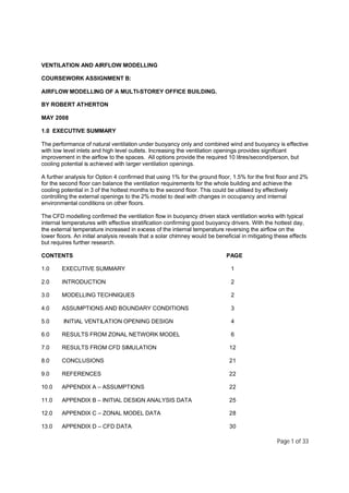
30. 13.0 APPENDIX D – CFD DATA
The ventilation flow rates for the 21 degree day, June 13 at 15:30 are indicated in Table D1
Table D1: Ventilation flow rates at openings
13 June at 15:30
North East South West
GF (m3/s) 0.1132 0.1132 0.2265
FF (m3/s) 0.0863 0.0863 0.1726
SF (m3/s) 0.3619
Stack (m3/s) -0.3496 -0.4661 -0.3496
The ventilation flow rates for the hottest day, May 14 at 17:30 are indicated in Table D2
Table D2: Ventilation flow rates at openings
14 May at 17:30
North East South West
GF (m3/s) -0.1057 -0.1057 -0.2113
FF (m3/s) -0.0905 -0.0905 -0.1813
SF (m3/s) 60.5
Stack (m3/s) 0.2019 0.2692 0.2019
o
Figure D1: CFD Grid Statistics for 21 C Day
Page 30 of 33

31. o
Figure D1: MicroFlo Monitor Output for 21 C Day
Figure D3: Mesh layout for both times prior to simulation
Note the thin horizontal line from left to right generated by the partition. This is enlarged in figure D4
below:
Page 31 of 33

32. Figure D4: Enlarged Mesh layout around partition
Figure D5: CFD Grid Statistics for Hottest Day
Page 32 of 33

33. Figure D6: MicroFlo Monitor Output for Hottest day
Figure D7: Image of solar chimney
Page 33 of 33