1. 1
Power At Sea: A Naval Power Dataset, 1865-2011
Brian Crisher
bcrisher@gmail.com
Florida State University
Mark Souva
msouva@fsu.edu
Florida State University
Abstract
Naval power is a crucial element of state power, yet existing naval datasets are limited to a small
number of states and ship types. Here we present 146 years of naval data on all the world’s
navies from 1865 to 2011. The creation of this country-year dataset focuses on warships that can
use kinetic force to inflict damage on other structures or peoples. As such, the dataset captures
naval power in terms of ship types and available firepower. This paper introduces the country-
year data, describes variables of interest that can be used in either country-year studies or dyadic
studies, and suggests potential questions of interest that scholars could explore using the naval
power dataset.
Word Count: 6537
2. 2
“A good navy is not a provocation to war. It is the surest guaranty of peace.”
– President Theodore Roosevelt, 2 December 1902, Second State of the Union
Section 1: Introduction
Strong states have the ability to project power beyond their own borders. When the
United States wishes to flex its military muscles abroad it sends a Carrier Strike Group
consisting of an aircraft carrier, at least one cruiser, two or more destroyers/frigates, submarines,
and logistical ships. Such a display of naval power is troubling for those whom are targeted by it,
but it is also the envy of other states who wish to have similar capabilities. As such, the
development of a formidable naval force plays a key role in power projection.
While the United States has enjoyed an unprecedented dominance of the world’s oceans
since the end of World War II, other states are beginning to devote more resources to the
development of naval strength. India has launched a nuclear attack submarine it bought from
Russia (INS Chakra), has a domestically produced nuclear ballistic submarine undergoing sea
trials (INS Arihant), is preparing to launch an aircraft carrier purchased from Russia (INS
Vikramaditya), and is also domestically building another aircraft carrier (INS Vikrant). The
launching of China’s first aircraft carrier, the ex-Soviet carrier Varyag, has increased tensions in
the South China Sea. Additionally, the British are constructing two new aircraft carriers – the
HMS Queen Elizabeth and HMS Prince of Wales. Moreover, ever vigilante of keeping their
place as the top naval power in the world, the US is currently developing a new class of aircraft
carriers set to replace the aging Nimitz class carriers, with the USS Gerald R. Ford set to launch
in 2015. As we move deeper into the 21st
Century, naval strength remains a key focus in the
plans of great and aspiring powers alike.
3. 3
Despite the prominence of naval power and its importance for understanding foreign
policy and international interactions, the academic community lacks a dataset on each state’s
naval capabilities. The foremost academic source of naval data comes from the work of
Modelski and Thompson (1988), yet this data is limited to the great powers, only includes the
most important warships in a given period, and ends in 1993.1
Rather than focusing on the
strongest states in the system and the strongest naval ships of the time, we have collected data on
all the world’s navies and all ships that have the capability of inflicting significant damage on
both land and sea targets for the period 1865 to 2011. The data we introduce here includes five
variables: state naval strength, aircraft carriers, battleships, submarines, and ballistic missile
submarines. Each is measured annually from 1865-2011.
The naval data we present here has numerous applications. For instance, the study of
arms races is a popular topic in international relations, and a few studies have focused
particularly on naval arms races (Bolks and Stoll 2000; Levy and Thompson 2010). Yet, these
studies only focus on the major powers. Even minor states are concerned about the naval strength
of enemies that are not traditionally considered major powers: witness the reaction of Israel to
the entrance of an Iranian destroyer into the Mediterranean Sea in February 2012. This dataset
could also help explain the likelihood of non-contiguous conflict. While the study of why
neighbors fight remains a popular topic (Vasquez 1995; Reed and Chiba 2010), fighting beyond
ones immediate borders is quite difficult (Bueno de Mesquita 1981). As such, a dataset whose
primary focus is on military capabilities that can be used to project power over great distances
will be useful to exploring the links between distance and conflict. Arms races and non-
contiguous conflict are only two of many topics for which this data will prove useful.
1
While the data presented by Modelski and Thompson (1988) ends in 1993, the last five years of data are actually
estimates based on knowledge of construction plans in 1988 (see Modelski and Thompson 1988, 90).
4. 4
Section 2: Measuring State Naval Power
Our primary concept of interest is state naval power, which we define as a state's ability
to use sea-based weapons to inflict physical damage on other states' people, territory, structures,
and weapons systems. There are several possible approaches to creating a single indicator of
each state’s naval power. One possibility is to focus on displacement. Here, one would sum the
displacement (in terms of tonnage) of all ships in a state’s inventory. While the largest ships –
that is, those with the most displacement – tend to have the most firepower, over time the
relationship between displacement and firepower becomes weak.2
Another option is to focus
more directly on weapons systems. To this end, one might sum the number of guns on all ships
in a state’s inventory. However, basing a measure solely on the number of guns fails to
acknowledge that not all guns are equal. Around the turn of the twentieth century, for example,
one would find that some ships have 12-inch guns while others have 8-inch guns. The
introduction of the submarine and aircraft carrier also make an exclusive focus on the number of
guns less useful.
Ideally, a measure of naval power would count every ship and have a perfect assessment
of each ship’s ability to inflict damage on an adversary’s territory or weapons systems. Such an
assessment would consider a ship’s displacement, weapons systems, total firepower, speed,
armor, and maneuverability. Unfortunately, this is not practical. The variation among the many
warships that have sailed the world’s waters in the last two centuries is too great to permit such
an assessment. As the primary purpose of a warship is to employ kinetic force to inflict damage
2
For example, in 1908 the Germans launched the SMS Blücher with a displacement of 17,250 tons and in 1909 the
Austro-Hungarian Navy launched the SMS Radetsky with a displacement of 15,847 tons. Based on displacement
alone, one might think the Blücher was the more powerful ship. However, the Blücher had 8.5-inch primary guns
while the Radetsky had 12-inch primary guns.
5. 5
on other structures or people, we opt for a measure that focuses on ship types and firepower.
Specifically, we classify all ships into a tier and record the number of ships in each tier for each
state. We propose a six-step-process to determine a state's sea power.
Data Sources
Prior to the discussion of the six-steps we should note that our primary source for data is
'Conway’s All the World’s Fighting Ships’ (Chesnau and Kolesnik 1979; Chesnau, 1980;
Gardiner and Gray, 1985; Gardiner, Chumbley, and Budzbon, 1995). We have also examined
Modelski and Thompson (1988), who draw primarily on Conway for the post 1865 period. The
Conway series ends in 1995. After 1995, our primary data source is “The Military Balance”
published by the Institute for Strategic Studies. There are two options for recording the first year
of a ship, the launch date and the service date. For a large portion of the ships included in the
Conway series, the launch date rather than the service date is available. As such we opt for the
launch date because of data availability. The primary difference between the two sources of data
deals with determining the first year a ship is active. While we use the launch date from the
Conway series, the Military Balance uses the service date (i.e., when a ship is commissioned).3
This results in some disparity between the two sources of data as we transition from the Conway
series in 1995, to the Military Balance journal in 1996. However, the disparity is minimal and is
resolved in the data within a few years.
Step 1: Distinguishing Naval Periods
3
For instance, the USS John C. Stennis - a Nimitz-class aircraft carrier - was launched in 1993, but commissioned in
1995. Therefore, based on the Conway series, we would consider the ship active in 1993 and 1994, but the Military
Balance journal would not consider the ship active until 1995. However, by 1995, the two sources of data would be
in agreement. Hence, the disparity is rather short lived.
6. 6
Naval technology has changed dramatically over time. For example, a pre-Dreadnought
battleship is not the most capable ship type in 1910 (the super-Dreadnaught class battleships are)
but compared to the premier warships twenty years earlier, it is at least as capable. Further, as we
previously noted, no single dimension allows for a perfect distinction between warships. Because
of changes in naval technology and the multiple dimensions that comprise warship capability, we
distinguish between different naval periods. A new naval period occurs with the emergence of a
new war fighting technology that gives the actor with the technology a significant military
advantage in head-to-head combat. In other words, a new naval period occurs when the most
dominant type of warship in the previous year is no longer dominant in the current year. Drawing
on the Conway series and Modelski and Thompson (1988), we identify five naval periods.
Our first period extends from 1860 to 1879. This is a transitional period as ship designers
began coming to grips with the technological leaps in terms of hulls, guns, and munitions. Hulls
were made thicker, sometimes out of iron and sometimes out of wood. For instance, the HMS
Agamemnon was launched in 1879 and displaced 8,510 tons. The Agamemnon’s relatively large
displacement was due both to the increase in armor she carried, and also the four 12.5 inch
muzzle-loading guns mounted in two separate turrets. Nevertheless, while heavier guns with
longer ranges and more explosive shells were placed on board in other ships, maneuverability
was greatly compromised due to poor ship design making them easy targets for faster ships with
heavy weapons.
Around 1880, the pre-Dreadnought emerges as the dominant warship. This begins our
second period that extends through 1905. An example of a pre-Dreadnought from the period is
the British HMS Royal Sovereign launched in 1891. Whereas the Agamemnon displaced 8,510
tons, the Royal Sovereign displaced 15,580 tons. Additionally, the primary guns of the Royal
7. 7
Sovereign were four 13.5 inch breech-loading guns capable of firing a 1,250 pound shell 12,000
yards, while the guns of the Agamemnon could only reach 6,500 yards. Lastly, despite being
vastly heavier than the Agamemnon, the Royal Sovereign had a maximum speed of 15.7 knots:
2.7 knots faster than the Agamemnon. In sum, the pre-Dreadnoughts were faster, heavier, and
more powerful than the battleships of the preceding period.
Period three covers the years 1906 to 1945. The launch of the HMS Dreadnought in 1906
ushered in the era of the battleship. The Dreadnought at its launching was the fastest battleship
in the world and could reach a speed of 21 knots (roughly 24 mph). Additionally, she displaced
over 20,000 tons when fully loaded and was armed with ten 12-inch guns. Another notable
battleship of this period was the German battleship Bismarck. At the time of its launch in 1939,
the Bismarck displaced over 50,000 tons and carried eight 15-inch guns. These 15-inch guns
were capable of firing 1,800 pound shells. Clearly, during this time battleships became bigger
and more powerful.
While this period marks the height of the battleships, other developments begin to alter
the naval landscape. The first development is the improvement of torpedo technology. In the
Russo-Japanese War, the torpedo played a prominent role for the first time in naval history. The
Russian battleship, Knyaz Suvorov became the first ever battleship to be sunk by torpedoes.
Torpedoes would also sink two armored cruisers and two destroyers during the war.
Additionally, torpedoes in various naval battles would damage dozens of other warships.
Similarly, the Kaiserliche Marine found that the improvement of torpedoes along with the
development of submarines were an effective weapon in the North Atlantic during World War I.
This period also saw the development of the aircraft carrier, which began to displace the
battleship as the capital warship during World War II. The worth of the aircraft carrier was
8. 8
shown during the sinking of the Bismarck. In a battle with the HMS Hood, one of Great Britain’s
major battle cruisers, the Bismarck sank the Hood and proceeded to head back to port for repairs.
However, torpedo-bombers launched from the HMS Royal Ark intercepted the Bismarck and
badly damaged her rudders, making her virtually unmaneuverable. This allowed other British
battleships to catch up, and eventually sink the Bismarck.
Period four is the first post-World War II period and extends from 1946 to 1958. As the
primary naval power in this period, the US Navy focused on projecting power inland. This leads
to an era where technological advances in armaments outpace advances in ship design – notably
the improvement in missile technology. For instance, in the early 1950s, the US developed the
Terrier as an effective medium-range surface-to-air missile that could be used to defend against
air attacks using radar guidance systems. Shortly afterwards, the Soviet’s launched their first
naval surface-to-air missile with the Berkut. These developments began the trend of missiles
replacing the traditional anti-aircraft guns that were the primary form of air defense during
World War II.
Lastly, period five deals with warships between 1959 and 2011. Two major technological
innovations mark the beginning of this final period. Both of these innovations highlight the US
Navy’s focus on using the navy to project power inland in the post-WWII world. The first occurs
in 1959 with the launching of the George Washington class nuclear submarines. These are the
first submarines to carry Polaris nuclear missiles. Additionally, the launch of the USS Enterprise
in 1960 marked the launch of the first nuclear powered aircraft carrier. Ships could now inflict an
incredible amount of damage on an enemy state and stay afloat or submerged as long as they had
the necessary supplies to sustain their crew. These innovations create a natural cut-off point to
mark the late period of naval technology.
9. 9
Step Two: Recording Individual Ships
After establishing the naval periods, we record all ships and their respective ship type that
meet minimum criteria. Periods one (1865-1879) and two (1880-1905) involve the least variation
among the types of warships available to all the world’s navies. As such, our minimum criterion
for recording a ship is straightforward for these two periods. In period one, we record all ships if
they displace at least 1,000 tons. For period two we add a gun size requirement and record all
ships if they displace at least 2,000 tons and have a 5-inch primary gun or greater. Due to the
lack of variation in ship types in these periods, we only record a ship’s displacement, not their
ship type.
By period three (1906-1947), as we noted previously, the landscape of naval technology
had been dramatically altered. Because of this, there was a need to alter our minimum criteria for
recording ships as well. In particular, we have minimum criteria for aircraft carriers, non-carrier
warships, and submarines. We record all aircraft carriers that are designated as such. However,
when recording the ship type for these carriers, we make a distinction between major and minor
aircraft carriers.4
Major aircraft carriers have at least 10,000 tons displacement while minor
aircraft carriers have less than 10,000 tons displacement. Next we record all submarines that are
designated as such. In this case we consider submarines that displace at least 1,000 tons
submerged and have four torpedo tubes as major, while submarines that displace less than 1,000
tons submerged are considered minor. Lastly, we record all non-carrier warships that have at
least 2,000 tons displacement and 5-inch guns, or ships with 1,000 tons of displacement and at
4
The Conway series makes a similar distinction for other types of ships. For example, armored cruisers are either
classified as an armored cruiser or as light armored cruisers. Essentially, we are making the same distinction among
ship types as the Conway series but applying it to more ship types, (e.g., battleships, aircraft carriers, and
submarines).
10. 10
least 3 torpedo tubes. Among non-carrier warships we do distinguish between major and minor
battleships. Ships that are designated as battleships and have at least 20,000 tons of displacement
and 12-inch guns are considered major battleships, while battleships that do not meet these
requirements are considered minor battleships.
We record ships in period four (1947-1958) similar to period three. We have minimum
criteria for aircraft carriers, non-carrier warships, and submarines while making some additional
distinctions among certain ship types. Because there was little development in ship design during
this period, the coding system is similar that of period three, but with some increases in the
minimum displacements. Ships designated as aircraft carriers are recorded as a major aircraft
carrier if they displace at least 20,000 tons and have at least 10 jet fighters. Aircraft carriers with
less than 20,000 tons of displacement are considered minor aircraft carriers. Submarines with at
least 2,000 tons displacement submerged and four torpedo tubes are considered major
submarines, while submarines with less than 2,000 tons of displacement are considered minor.
Lastly, we record non-carrier warships that have at least 2,000 tons of displacement and 5-inch
guns or six torpedo tubes.5
In period five (1959-2011) we record aircraft carriers with at least 30,000 tons of
displacement and 10 jet fighters as major aircraft carriers, while minor aircraft carriers are those
with less than 30,000 tons of displacement. For non-carrier warships we record ships that have at
least 3,000 tons of displacement and 5-inch guns, at least 6 torpedo tubes, or missile capability.
In terms of submarines, we consider those submarines that are capable of launching nuclear-
ballistic missiles separately from other submarines. However, conventional submarines with at
least 3,000 tons of displacement submerged and four torpedo tubes are classified as major
5
We drop the distinction between major and minor battleships in this period as no battleships were launched in this
period.
11. 11
submarines, while submarines with between 2,000-3,000 tons displacement submerged and four
torpedo tubes are minor submarines.
Step Three: Calculating Per Salvo Payloads for each Ship Type
The next step in calculating state naval power is to calculate the potential per salvo
payload for each type of ship identified in step two. Specifically, for each ship type identified
(i.e., battleship, destroyer, submarine…etc) we calculate that ship’s potential per salvo payload
in pounds. Table 1 provides an example. For period three, one of the ship types identified is
major battleships, with the USS Arizona being a typical battleship of the period. She had at her
disposal twelve 14-inch guns each capable of firing a 1,500 pound shell. In addition, she had
twenty-two 5-inch guns each capable of firing a 55 pound shell, and two torpedo tubes each
capable of firing a torpedo with a 900 pound warhead. Taken together, the USS Arizona could
fire 20,100 pounds of destructive power with a given salvo. Accordingly, we argue that a typical
major battleship in period three could fire 20,110 pounds per salvo.6
We perform this calculation
for every ship type identified in step two.
[Table I in here]
Step Four: The Period-Tier System
We address the multidimensionality challenge by classifying ships into tiers within a
naval period. This will allow us to weight some ships more than others. Table 2 shows the five
6
It would be ideal to do this for every ship that is classified as a major battleship in period three, but the amount of
time that would be required to complete the task makes it impractical.
12. 12
time periods and one of the representative ship types we use to calculate the average potential
per salvo payload for each tier from step three.7
Next, we explain our tier demarcation choices.
Period one (1865-1879) is the most difficult era to code. Indeed, Modelski and Thompson
(1988: 74) write that, “Even the strongest navy of the period has been described as being
composed of twenty-five different types of battleships. Such circumstances pose nearly-
overwhelming odds against quantification and comparison both then and now.” We distinguish
between two tiers of ships in this period. Tier 1 ships are the major war-fighting ships of the era.
We contend that tier 1 ships in this period are those with a displacement of at least 5,500 tons.
Ships with a displacement between 1,000-4,499 tons are considered tier 2 ships. This is by no
means the most appealing solution to the problem of this period, but it is the best realistic
solution. Moreover, an examination of volume 1 of the Conway series suggests this is the criteria
the editors use to classify ‘capital ships.’
[Table II in here]
In period two (1880-1905) we also create two tiers of ships, but now tier 1 ships must
meet two criteria, displacement and gun size. Generally, tier 1 ships at this time are pre-
Dreadnoughts. While they vary in displacement and gun size, a majority of pre-Dreadnoughts
had at least 8,500 tons of displacement and guns that were a minimum of 12 inches in bore
diameter. This serves as our criteria for a tier 1 in this period. We added gun size here because
there are a number of ships that displace more than 8,500 tons, but their firepower and armor
were inferior to the pre-Dreadnoughts. For instance, near the end of the period states began to
develop armored cruisers such as the USS Washington that sought a balance between speed and
firepower. The USS Washington was an armored cruiser that displaced 15,712 tons, had 10-inch
7
Readers will note the absence of ballistic nuclear missile submarines from this table. They are not included in this
particular classification as we are interested in quantifying conventional forces. Nevertheless, the dataset includes a
binary variable indicating whether a state has ballistic missile submarines in a given year.
13. 13
primary guns, and had a maximum speed of 22 knots. Yet, the Washington did not have the
firepower for a one-on-one battle with a pre-Dreadnought. Hence, tier 2 warships must meet
minimum criteria of 2,000 tons displacement and carry guns that are at least 5-inches in bore
diameter. Many ships that do not meet the tier 2 minimums were not meant to travel beyond
rivers (paddleboats) or beyond shallow coastal waters (shallow-draft monitors). Other ships not
meeting the tier 2 thresholds lacked the armor to withstand an attack from even minor ships, or
the necessary gun size to go on the offensive against other minor ships. We do not record ships
below the tier 2 cutoffs.
For periods three through five we propose a system that creates a hierarchy of ships based
on the available firepower for a given ship calculated in step three. Such a system is
advantageous as there is more variation among ships types in these periods. For instance, in these
periods the aircraft carrier and submarines must be taken into account. For these periods, we take
the potential per salvo payload for every ship type calculated in step three and rank the ships
from greatest to least in terms of salvo payload. From here, we place each ship type into one of
six tiers. After doing this for the years 1906-2011, we have six total tiers in each respective
period.
Step Five: The Multiplier System
The tier system allows us to weight some ships more than others. The weight, or
multiplier, for each tier is its percentage of the total average period payload. Specifically, we
divide the average payload for a given tier by the total average payload in that period calculated
in step three. Note that for this it is necessary to calculate an average per salvo payload for each
tier. In other words, for each tier we average the payloads, calculated in step three, across all the
14. 14
ship types placed in said tier. After this, we sum the averages for all six tiers to calculate the
average period payload. For example, in period five, we calculate the average payload for a tier 1
ship as 411,740 pounds and the total average payload for all tiers in period five as 621,002.
Dividing the first into the second gives 0.66. This means that, generally speaking, tier 1 ships
account for 66% of the global naval firepower in period five. We multiply this number by 10 and
get a multiplier for individual ships in this tier: in this case it is 6.6. We calculate multipliers for
each tier for each period.
Step Six: Recording the Total Number of Active Ships in Each Tier
Next, we need a count of the total number of active warships in each tier for each state in
a given year. The difficulty of creating such a count is that our period demarcations are artificial,
yet a ship’s life can span multiple periods. For instance, we make a distinction between 1860-
1879 and 1880-1905. If a ship is coded as a tier 1 ship in the former period, what is its status in
the latter period? Modelski and Thompson (1988) simply drop the ship from consideration; a tier
1 ship in 1879 would drop out of the data set in 1880. We believe there is an alternative way for
dealing with this issue. A warship still in commission can serve as a military asset even if it is
slightly outdated. Additionally, one must consider that it takes time for older technology to phase
out as states incorporate the latest technology into their ship designs. However, there does
become a time when ships are outclassed to the point that they no longer serve a military purpose
and frequently these ships are hulked, stripped of useful parts, or converted into trainer ships.
Our task is made slightly more difficult as the data structure for periods one and two are
different from the data structures for periods three through five. In periods one and two, we only
have the designation of tier 1 and 2 ships, while the other periods have the six tier system as
15. 15
described above. As such, our solution to the overlap problem is unique to each transition period
with ships dropping in tier rankings dependent upon their potential payload calculated in step
three. A full outline of the transition rules can be found in the online appendix.
Section 3: Key Variables
The primary variable of interest in this data is state naval strength. In addition, we include binary
variables for a variety of noteworthy ship types: aircraft carrier, battleship, nuclear ballistic
missile submarine, and submarine. Each of these is equal to one in a given year if a state
possesses this type of warship, zero otherwise.
3.1 Naval Strength
To create a measure of state naval strength, we draw on the calculations performed in
steps one to six. The variable Naval Strength equals the sum of the number of ships in each tier
(stage five) multiplied by their respective multiplier. As an example, we calculate the Naval
Strength for the US in 1995. In 1995, the US had 14 tier 1, 40 tier 3, 89 tier 4, 104 tier 5, and 1
tier 6 ships. Hence, for the US in 1995, Naval Strength = (14*6.6) + (40*0.9) + (89*0.49) +
(104*0.08) + (1*0.01), which equals 180.74. The advantage of the multiplier system is that it
gives greater weight to the more powerful naval ships. In other words, the multipliers allow the
more powerful ships to have a greater influence on a state’s total naval strength.
3.2 Naval Proportion
We can use the Naval Strength variable to create an additional variable that gives insight
into a state’s naval power. By taking into consideration the total naval strength available in the
international system in a given year, we can calculate what proportion of naval power a state’s
16. 16
navy accounts for in that particular year. The calculation is quite similar to how the Correlates of
War Composite Indicator of National Capability (COW CINC) is calculated (Singer, Bremer,
and Suckey, 1972). As such, Naval Proportion is calculated as:
, where i = state, and j = year (1)
This variable results in a value between 0 and 1 and represents a state’s percentage of world
naval capability for a given year. For instance, in 1957 and 1958 the US accounted for a
staggering 70% of the world’s naval power. As a state develops a larger navy in relation to other
states, this number will rise. However, as other states develop their navies this value could drop
if a state is not building more ships to maintain its advantage. This measure, then, not only
allows us to track how powerful a state’s navy is, but also how powerful it is in relation to the
other navies of the world.
Section 4: Discussion of Data
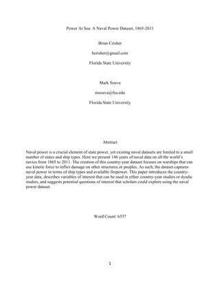
Who are the strongest navies in the world system between 1865 and 2011? From our
measures of naval power we can rank the world’s navies from strongest to weakest. Not
surprisingly, one of two states has always ranked as the strongest navy: Great Britain and the
United States. Figure 1 shows the top five powers based on Naval Proportion for selected years
from 1870 to 2010. The rankings of the top five powers by decade can be found in Table 6 in the
appendix.
Figure 1 not only lists the five most powerful navies for selected years, it shows the gap
that can exist even among the most powerful navies. For instance, in the 1870s and 1880s the
French navy was not much weaker than the British. However, by the turn of the century, the
17. 17
British navy was clearly the strongest, nearly doubling France's percentage of the world’s naval
power. However, by the signing of the Washington Naval Treaty in 1922, the United States was
the world’s strongest naval power. Just like in the case of the British, here we can see a gap
growing between the US and the rest of the world’s navies – particularly during the post-World
War II period.
Figure 1: Top 5 Naval Powers based on Naval Proportion
We can verify this trend by plotting the power of the British and US navies. Figure 2
shows Naval Proportion for the US and Britain from 1865 to 2011. Leading into World War I,
the British were at the height of their naval power. Yet, Figure 2 shows that by the signing of the
Washington Naval Treaty the power of the US navy had surpassed that of the British navy. The
figure also shows that in the second half of the twentieth century, the US enjoyed preeminence in
naval power that the British could only dream about in the nineteenth century.
Netherlands
Russia
USA
France
UK
1870
%
0.00
0.05
0.10
0.15
0.20
0.25
USA
Russia
Germany
France
UK
1900
%
0.00
0.05
0.10
0.15
0.20
0.25
0.30
Italy
France
Japan
UK
USA
1930
%
0.00
0.05
0.10
0.15
0.20
0.25
0.30
Netherlands
France
UK
Russia
USA
1960
%
0.0
0.1
0.2
0.3
0.4
India
UK
France
Russia
USA
1990
%
0.0
0.1
0.2
0.3
0.4
UK
France
China
Russia
USA
2010
%
0.0
0.1
0.2
0.3
0.4
0.5
18. 18
Figure 2: US and UK Naval Proportion 1865-2011
One of the most popular measures of military capability is the Composite Indicator of
National Capabilities (CINC) from the Correlates of War (COW) project. How well does our
measure of naval strength correlate with the COW composite capabilities components? Figure 4
shows the correlations between our measures of naval power and the COW capability
components. From 1865 to 2011, naval strength correlates at 0.73 with the COW indicator of
military power.8
This highlights that the strongest states in the world tend to have large and
technologically advanced navies. We argue that the less than perfect correlation between naval
strength and COWCINC is to be expected and may suggest that naval strength is a better
measure if one wants to explore certain theoretically interesting questions, such as the
determinants of non-contiguous conflict.
8
Readers should also note the rather weak correlation between our measures of naval strength and military
expenditure. This suggests military expenditures can be applied to a wide range of military systems. A more
nuanced understanding of arms races would require direct measures of military capabilities. Our measure of naval
strength could help to achieve such an understanding.
0
.2.4.6.8
NavalProportion
1870 1890 1910 1930 1950 1970 1990 2010
1921
Year
UK USA
UK vs USA
Changing of the Guards
19. 19
Figure 3: Correlations
What these figures suggest is that the COWCINC might not be the appropriate measure
of military power in all situations. For questions that need a valid measure of naval power, the
COWCINC scores should not be used as a proxy. COWCINC does not directly measure
capabilities; it measures factors that influence the production of military capabilities. This makes
COWCINC a latent measure of military power. Naval strength is a direct measure of a particular
military capability. As such, it should not correlate perfectly with the COWCINC. If the decision
to militarily threaten or attack another state abroad is more a function of one’s present naval
capabilities than one’s military potential, then naval strength may well be a better indicator for
understanding the onset and initiation of militarized disputes.
Section 5: Application: Explaining Non-Contiguous Militarized Conflict, 1865-2000
20. 20
One use for this data is to explain the occurrence of militarized conflict between states,
particularly conflicts between non-contiguous states as contiguous states can, of course, inflict
harm on each other even if they lack naval power. We estimated four models of non-contiguous
MIDs, two with the COW CINC power ratio and two with our naval power ratio.9
Figure 7
shows the maximum likelihood estimates and confidence intervals. We find that generally there
is a positive relationship between power and MID onset. However, the naval power ratio has a
larger substantive influence on the likelihood of a non-directed dyad experiencing a MID than
the CINC power ratio. To fully appreciate the differing influence of these variables, Clarify
simulations (King, Tomz, and Wittenberg, 2000) were ran to see how increasing the respective
variable from the 5th
to 95th
percentile would influence the likelihood of conflict using the 1865-
2000 models. A change from a CINC power ratio score at the 5th
percentile to one at the 95th
percentile increases the likelihood of a MID initiation by about 88%. A similar change for the
naval power ratio increases the likelihood of a MID initiation by 2346%! States with more naval
power are much more likely to initiate MIDs against states with weaker navies. The naval ratio
coefficients show that the strong tend to pick on the weak.10
9
The full results for all models can be found in the online appendix. The variable was calculated in a similar fashion
as the COW CINC power ratio – it’s construction can also be found in the online appendix.
10
For a more realistic example, we ran simulations for the likelihood of conflict based on the current naval strengths
of China and Indonesia and the likelihood of conflict for when China's aircraft carrier becomes active. In the
simulations, China having an active aircraft carrier increased the likelihood that this dyad experiences conflict by
50% - a substantively significant increase.
21. 21
Figure 4: Non-Directed Dyad Model Results
Figure 7 also displays estimates and confidence intervals for this relationship in the post-
World War II period. Here we also find an interesting result. We see that in the post-WWII
period, there is no statistical relationship between the CINC power ratio variable and the onset of
a MID. However, our variable, Navy Power Ratio is statistically and positively associated with a
MID. As this ratio increases, meaning the balance of power in the dyad becomes more uneven,
the likelihood of a MID increases. The positive relationship between the Naval Power Ratio and
the onset of a MID is particularly noteworthy as the standard finding in empirical research on
interstate conflict is that conflict is more likely under the condition of power parity than power
preponderance. At least when it comes to naval power and non-contiguous conflict, we find the
opposite.11
Section 6: Conclusion
11
The correlation between the COW power ratio and the naval power ratio variables is 0.24 for non-contiguous
dyads and 0.4 for contiguous ones.
-2 0 2 4 6 8
Power Ratio
Navy Ratio
Non-contiguous MID Initiation
-2 0 2 4 6 8
1865-2000
1946-2000
22. 22
The naval power dataset we present here includes five variables—state naval strength
(continuous), aircraft carriers (binary), battleships (binary), submarines (binary), ballistic missile
submarines (binary)—measured annually from 1865-2011. We believe scholars will find this
data applicable to numerous topics in international relations and foreign policy. In section four
we argued that our naval data is substantively different from the COW CINC scores. We
emphasized this point in section five while exploring one potential application of the naval data –
understanding non-contiguous conflict. Not only was our measure of naval balance of power a
more powerful predictor of conflict onset, it remained positive and significant in the post-World
War II period while the CINC power ratio measure was insignificant. This finding represents just
one potential area of research that could benefit from the dataset presented in this study.
23. 23
Bibliography
Bolks, Sean, and Richard J. Stoll. 2000. "The Arms Acquisition Process: The Effect of Internal
and External Constraints on Arms Race Dynamics." Journal of Conflict Resolution 44(5):
580-603.
Bueno de Mesquita, Bruce. 1981. The War Trap. Yale: Yale University Press.
Chesneau, Roger, and Eugene M. Kolesnik. 1979. Conway’s All the World’s Fighting Ships,
1860-1905. London: Conway Maritime Press.
Chesneau, Roger. 1980. Conway’s All the World’s Fighting Ships, 1922-1946. London: Conway
Maritime Press.
Gardiner, Robert, Randal Gray. 1985. Conway’s All the World’s Fighting Ships, 1906-1921.
London: Conway Maritime Press.
Gardiner, Robert, Stephen Chumbley, and Przemysaw Budzbon. 1995. Conway’s All the World’s
Fighting Ships, 1947-1995. Annapolis: Naval Institute Press.
Levy, Jack S. and William R. Thompson. 2010. "Balancing on Land and Sea: Do States Ally
Against the Leading Global Power?" International Security 35(1): 7-43.
Massie, Robert K. 1991. Dreadnought: Britain, Germany, and the Coming of the Great War.
New York: Ballantine Books.
Modelski, George and William R. Thompson. 1988. Seapower in Global Politics, 1494-1993.
Seattle: University of Washington Press.
Reed, William and Daina Chiba. 2010. "Decomposing the Relationship Between Contiguity and
Militarized Conflict." American Journal of Political Science 54(1): 61-73.
Singer, J. David, Stuart Bremer, and John Stuckey. 1972. “Capability Distribution,
Uncertainty, and Major Power War, 1820-1965.” in Bruce Russett (ed) Peace, War, and
Numbers, Beverly Hills: Sage, 19-48.
Vasquez, John A. 1995. "Why Do Neighbors Fight? Proximity, Interaction, or Territoriality."
Journal of Peace Research 32(3): 277-293.
24. 24
Table I: Break Down of the USS Arizona
Ship
Base
Primary
Gun
Secondary
Gun
Size of
Salvo
(lbs)
Torpedo Tubes Warhead
Weight
Per salvo
payload
Battleship Arizona 14in x 12 5in x 22 19210 2 900 20110
Table II: Period and Tier System Overview
Period Tier Characteristic Ship*
1 (1865-1879) 1 Battleship
2 Corvette
2 (1880-1905) 1 Pre-dreadnought
2 Cruiser
3 (1906-1946) 1 Battleship
2 Battlecruiser
3 Cruiser
4 Submarine (major)
5 Monitor
6 Torpedo Boat
4 (1947-1958) 1 Aircraft Carrier (major)
2 Aircraft Carrier (minor)
3 Cruiser
4 Submarine (major)
5 Submarine (minor)
6 Command Ship
5 (1959-2011) 1 Aircraft Carrier (major)
2 Air Capable Ship
3 Cruiser
4 Submarine (major)
5 Destroyer
6 ---
* In any given tier there may be more than one type of ship. See Appendix for a list of all ships
in tiers 3, 4, and 5.
27. 27
Section B: Transition Rules
The transition rules are as follows:
Period 1 to Period 2:
Tier 1 Ships – A tier 1 ship will remain so for an additional five years. After that,
it will be considered a tier 2 ship for another ten years, or it is decommissioned,
whichever comes first.
Tier 2 Ships – A tier 2 ship will remain so for an additional ten years, or it is
decommissioned, whichever comes first.
Period 2 to Period 3:
Tier 1 Ships – A tier 1 ship will be considered a tier 3 ship for a period of five
years, then a tier 4 ship for five years, and finally a tier 5 ship for five years. If the
ship is still in commission after these fifteen years, it is dropped from the data
set.12
Tier 2 Ships – A tier 2 ship will be considered a tier 5 ship for a period of five
years, and then a tier 6 ship for another five years. If the ship is still in
commission after these ten years, it is dropped from the data set.
Period 3 ships to Period 4 and Period 5:13
Tier 1 Ships – These ships will be considered a tier 2 ship in period four, and a
tier 3 ship in period five.
Tier 2 Ships – These ships will be considered a tier 3 ship in period four, and a
tier 4 ship in period five.
Tier 3 Ships – These ships will be considered a tier 4 ship in period four, and a
tier 5 ship in period five.
Tier 4 Ships – These ships will be considered a tier 5 ship in period four, and a
tier 6 ship in period five.
Tier 5 Ships – Same as tier 4 Ships.
Tier 6 Ships – These ships will be considered a tier 6 ship in period four, and
dropped from the data set in period five.
12
The transition of a tier 1 ship in period two to a tier 3 ship in period three is based on the average payload. The
average payload for a period two tier 1 ship is 4140 pounds, which translates roughly to a tier 3 ship in period three
that has an average payload of 5543 pounds. A similar evaluation was made for period three tier 2 ships.
13
Similar to the transitions from period three to period four, the decisions to drop a ship from any given tier to
another during the overlap period is based on average payload.
28. 28
Period 4 ships to Period 5:
Tier 1 Ships – These ships will remain tier 1 ships in period five.
Tier 2 Ships – These ships will remain tier 2 ships in period five.
Tier 3 Ships – These ships will be considered a tier 4 ship in period five.
Tier 4 Ships – These ships will be considered a tier 5 ship in period five.
Tier 5 Ships – These ships will be considered a tier 6 ship in period five.
Tier 6 Ships – Same as tier 5 Ships.
To see how this transition scheme operates, we can track a ship that is consider a tier 1
ship in period two, but drops to a lower tier in period three. On July 23, 1903, the Royal British
Navy launched the HMS King Edward VII. She had 17,800 tons of displacement and had four
12-inch primary guns each capable of firing an 850 pound shell. Shortly afterwards, the British
launched the HMS Dreadnaught with her ten 12-inch guns, increased speed, and thicker armor.
Virtually overnight, the King Edward VII became obsolete.14
That being said, she still had
military worth. After all, there were still plenty of ships patrolling the seas that would want to
avoid being at the wrong end of her 12-inch guns. As such, we would consider the King Edward
VII to be a tier 3 ship for five years in period three. However, by 1910 the British launched the
HMS Orion to be the lead ship in their first class of super-dreadnoughts. The Orion had the same
speed as the Dreadnought, but heavier armor and ten 13.5-inch primary guns each capable of
firing a 1,400 pound shell. By 1911, the King Edward VII was no match for the latest class of
battleships that the British were producing. Yet still, we would consider her to be a tier 4 ship for
five years (starting in 1911), and a tier 5 ship for a further five years. If after this point (1920),
14
Not everyone in the British Admiralty was excited about the launching of the Dreadnaught. Admiral of the Fleet
Sir Frederick Richards argued that her launching meant that “The whole British Fleet was…morally scrapped and
labeled obsolete at the moment when it was at the zenith of its efficiency and equal not to two but practically to all
the other navies of the world combined.” (quoted in Massie (1991: 487))
29. 29
the ship was still in commission, it would be dropped from the data set. However, in this case,
the King Edward VII, sunk after being mined in 1916.15
We can also track a ship that was a tier 4 ship in period three, but drops to a tier 5 ship in
period four. During World War II, the US Navy launched the Gato-class submarines. They had a
submerged displacement of 2,090 tons and had 10 torpedo tubes. By the late 1940s the US had
launched the Tang-class submarines that incorporated state-of-the-art submarine technology.
These submarines had a submerged displacement of nearly 3,000 tons and had 8 torpedo tubes.
While the Tang-class had fewer torpedoes than the Gato-class, the Tang-class submarines could
dive up to 700 feet while the Gato-class could only dive up to 300 feet. Perhaps the most
important difference is that the Gato-class submarines could only make 9 knots submerged,
while the Tang-class could make 18.3 knots submerged. Hence, the Tang-class submarines could
dive deep and travel faster than the Gato-class submarines. Again, however, we feel that the
Gato-class submarines could serve a purpose despite being outdated and we would consider
them a tier 5 ship in period four.
15
The fate of the King Edward VII shows that even the British no longer considered her a major ship. These types of
ships often served at the head of the fleet in order to spot mines or strike them first in order to protect the higher
rated battleships.
30. 30
Section C: Top 5 Naval Powers by Decade
Country
Navy
Proportion
Naval
Strength Country
Navy
Proportion
Naval
Strength Country
Navy
Proportion
Naval
Strength
1870 1920 1970
United
Kingdom 0.26 374.4
United
Kingdom 0.32 446.76
United
States 0.42 186.17
France 0.21 311.6
United
States 0.26 372.48 Russia 0.25 105.45
United
States 0.12 186 Germany 0.1 137.26
United
Kingdom 0.08 32.12
Russia 0.07 95.1 France 0.09 123.23 France 0.07 27.34
Netherlands 0.05 68.2 Japan 0.08 106.99 Netherlands 0.02 7.1
1880 1930 1980
United
Kingdom 0.26 547.5
United
States 0.33 400.83
United
States 0.42 170.5
France 0.21 434.5
United
Kingdom 0.22 271.51 Russia 0.35 140.36
United
States 0.08 164.5 Japan 0.15 186.49 France 0.06 22.4
Germany 0.07 152.5 France 0.09 115.15
United
Kingdom 0.04 16.76
Russia 0.07 138 Italy 0.06 74.15 India 0.01 5.07
1890 1940 1990
United
Kingdom 0.29 315.5
United
States 0.25 448.14
United
States 0.49 216.27
France 0.19 211.5
United
Kingdom 0.22 391.58 Russia 0.34 149.65
Italy 0.09 101.5 Japan 0.19 343.42 France 0.04 17.25
Germany 0.07 84 France 0.08 148.29
United
Kingdom 0.04 16
Russia 0.07 74 Italy 0.07 129.78 India 0.02 7.03
1900 1950 2000
United
Kingdom 0.3 603.5
United
States 0.68 584.3
United
States 0.52 144.63
France 0.16 335.5
United
Kingdom 0.17 149.41 Russia 0.11 29.84
Germany 0.09 188 France 0.04 33.24
United
Kingdom 0.05 14.06
Russia 0.09 181.5 Russia 0.04 31.39 France 0.05 13.37
United
States 0.08 163.5 Argentina 0.01 10.55 China 0.04 11.89
1910 1960 2010
United
Kingdom 0.34 176.62
United
States 0.43 177.95
United
States 0.5 130.73
Germany 0.17 89.83 Russia 0.17 64.04 Russia 0.1 26.95
United
States 0.13 65.11
United
Kingdom 0.13 49.59 China 0.05 13.74
France 0.09 48.75 France 0.09 33.13 France 0.05 12.22
Japan 0.06 31.94 Netherlands 0.02 9
United
Kingdom 0.04 9.56
31. 31
Section D: Variable Coding for Multivariate Model
This section describes how we coded the variables in our multivariate model of non-
contiguous MID onset.
The dependent variable, MID onset, equals one for the first year of a new militarized
interstate dispute. Data generated by EUGene (version 3.204).
We considered a dyad contiguous if they are land adjacent or separated by no more than
400 miles of water. Contiguous dyads were dropped from the data so that the analysis was only
run on non-contiguous dyads.
The variable Naval Ratio is the ratio of the state with the largest Naval Strength divided
by the total Naval Strength for the dyad.
(2)
The variable Power Ratio is the ratio of the state with the largest COW CINC score
divided by the total CINC score for the dyad. Data generated by EUGene (version 3.204).
Allies equals one if the two states share a defense pact, neutrality pact, or entente, as
defined by the Correlates of War project, zero otherwise. Data generated by EUGene (version
3.204).
Alliance Portfolio Similarity is the unweighted global S score between the two states in
the dyad. Data generated by EUGene (version 3.204).
Ln(Distance) is the natural log of the great circle capital-to-capital distance. Data
generated by EUGene (version 3.204).
Peace Years is the count of the number of years since the last MID in this dyad. Splines
1-3 are cubic splines generated from the Peace Years variables (Beck, Katz, and Tucker, 1998).
32. 32
Section E: Multivariate Model Estimates of Non-Contiguous MID Onset
Model 1 Model 2 Model 3 Model 4
1865-2000 1865-2000 1946-2000 1946-2000
COWCAP Power Ratio 1.225* -0.079
(0.525) (0.500)
Navy Ratio 6.780*** 6.099***
(0.363) (0.446)
Alliance Portfolio -3.447*** -1.753*** -5.108*** -2.621***
(0.360) (0.293) (0.455) (0.403)
Allies 0.946*** 0.547** 1.501*** 0.746**
(0.222) (0.173) (0.295) (0.241)
Ln Distance -0.936*** -0.788*** -1.149*** -1.081***
(0.067) (0.067) (0.079) (0.087)
Peace Years -0.260*** -0.255*** -0.248*** -0.237***
(0.025) (0.024) (0.034) (0.033)
Spline 1 -0.001*** -0.001*** -0.001** -0.001**
(0.000) (0.000) (0.000) (0.000)
Spline 2 0.000*** 0.000*** 0.000 0.000
(0.000) (0.000) (0.000) (0.000)
Spline 3 0.000 0.000 0.000 0.000
(0.000) (0.000) (0.000) (0.000)
Constant 3.750*** -2.403** 7.196*** 0.769
(0.783) (0.747) (0.826) (0.982)
N 600808 600809 517317 517318
* p < 5%, ** p < 1%, *** p < 0.1%, two-tailed test. Standard errors clustered on the dyad.
33. 33
References
Beck, Nathaniel, Jonathan N. Katz and Richard Tucker. 1998. “Taking Time Seriously: Time-
Series-Cross-Section Analysis with a Binary Dependent Variable.” American Journal of
Political Science 42:1260-1288.
Bennett, D. Scott, and Allan Stam. 2000. “EUGene: A Conceptual Manual.” International
Interactions 26:179-204.