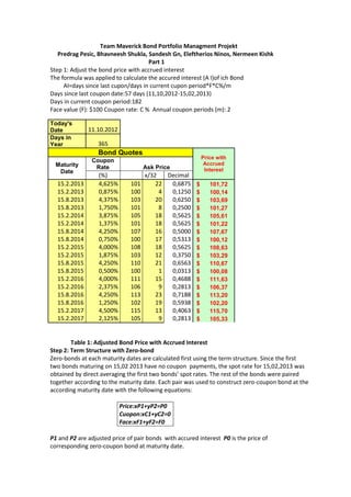
1. Team Maverick Bond Portfolio Managment Projekt
Predrag Pesic, Bhavneesh Shukla, Sandesh Gn, Eleftherios Ninos, Nermeen Kishk
Part 1
Step 1: Adjust the bond price with accrued interest
The formula was applied to calculate the accured interest (A I)of ich Bond
AI=days since last cupon/days in current cupon period*F*C%/m
Days since last coupon date:57 days (11,10,2012-15,02,2013)
Days in current coupon period:182
Face value (F): $100 Coupon rate: C % Annual coupon periods (m): 2
Today's
Date 11.10.2012
Days in
Year 365
Bond Quotes
Price with
Coupon
Maturity Accrued
Rate Ask Price Interest
Date
(%) x/32 Decimal
15.2.2013 4,625% 101 22 0,6875 $ 101,72
15.2.2013 0,875% 100 4 0,1250 $ 100,14
15.8.2013 4,375% 103 20 0,6250 $ 103,69
15.8.2013 1,750% 101 8 0,2500 $ 101,27
15.2.2014 3,875% 105 18 0,5625 $ 105,61
15.2.2014 1,375% 101 18 0,5625 $ 101,22
15.8.2014 4,250% 107 16 0,5000 $ 107,67
15.8.2014 0,750% 100 17 0,5313 $ 100,12
15.2.2015 4,000% 108 18 0,5625 $ 108,63
15.2.2015 1,875% 103 12 0,3750 $ 103,29
15.8.2015 4,250% 110 21 0,6563 $ 110,67
15.8.2015 0,500% 100 1 0,0313 $ 100,08
15.2.2016 4,000% 111 15 0,4688 $ 111,63
15.2.2016 2,375% 106 9 0,2813 $ 106,37
15.8.2016 4,250% 113 23 0,7188 $ 113,20
15.8.2016 1,250% 102 19 0,5938 $ 102,20
15.2.2017 4,500% 115 13 0,4063 $ 115,70
15.2.2017 2,125% 105 9 0,2813 $ 105,33
Table 1: Adjusted Bond Price with Accrued Interest
Step 2: Term Structure with Zero-bond
Zero-bonds at each maturity dates are calculated first using the term structure. Since the first
two bonds maturing on 15,02 2013 have no coupon payments, the spot rate for 15,02,2013 was
obtained by direct averaging the first two bonds’ spot rates. The rest of the bonds were paired
together according to the maturity date. Each pair was used to construct zero-coupon bond at the
according maturity date with the following equations:
Price:xP1+yP2=P0
Cuopon:xC1+yC2=0
Face:xF1+yF2=F0
P1 and P2 are adjusted price of pair bonds with accured interest P0 is the price of
corresponding zero-coupon bond at maturity date.

2. The spot rate St at each maturity date can be calculated with following equations:
P0=D(t) F0=exp(-Si*t)
St=in(F0/P0)/t
Zero Coupon Bonds with Face Value $100
Poly Derived
Short Rates
Maturity Spot Rates
Price of Zero Time to Maturity Spot Rate
Date
15.2.2013 $99,96 0,347945205 0,112% 0,093% 0,169%
15.8.2013 $99,67 0,843835616 0,396% 0,176% 0,282%
15.2.2014 $99,36 1,347945205 0,474% 0,227% 0,345%
15.8.2014 $99,04 1,843835616 0,524% 0,270% 0,442%
15.2.2015 $98,80 2,347945205 0,515% 0,326% 0,640%
15.8.2015 $98,61 2,843835616 0,491% 0,407% 0,965%
15.2.2016 $98,70 3,347945205 0,391% 0,525% 1,438%
15.8.2016 $97,96 3,846575342 0,536% 0,681% 2,030%
15.2.2017 $96,22 4,350684932 0,885% 0,876% 2,710%
Step 3: Term Structure with Polynomial
The spot rate at each maturity date can also be approximated by a 4th order polynomial
St=
D(t)=exp( *t)=exp(-( ))
The price from the polynomial approximation Qj(t) can be obtained by summing the discounted
coupon payments and face value of bond j using the corresponding D(t). In order to find the term
structure coefficients, we setup the following least squares optimization:
min
With constraint ao≥0 the term structure coefficients that minimizes the sum of square
we show in the Tabel 4
Term Structure Coefficients Sum of Squared Error
a0 0,0000026518253 1,06
a1 0,0031998339503
a2 -0,0017122129494
a3 0,0004826096945
a4 -0,0000348844366
Tabel 4

3. Step5a
Cash matching
with reinvestment
at zero rate
Portfolio
0
99,80413576
0
49,80850219
0
399,8128604
0
69,84034757
0
799,8429666
0
119,9179519
0
499,9209498
0
59,98031542
0
149,9840642
233032,2
CF from
Portfolio
10000
5000
40000
7000
80000
12000
50000
6000
15000
Step 5: Cash Matching of Liabilities
A) Simple Cash Matching: excess periodic cash flows are held at zero interest.
Main objective of cash matching is to minimize the portfolio cost
We contains
( +

4. Portfolio generated cash flow-ceash leaved for the next period≥liability
For the intermediate period (From 15,02,2013-15,08,2016)
( for j=2,…,8
Portfolio generated cash flow + previous excess – cash leaved for the next period ≥ liability
(From15,02,2016-15,02,2017)
(
Portfolio generated cash flow + previous excess ≥ liability
≥ 0 for j=1,2,…,8 Cash leaved for the next period ≥ 0
Step6 A. Present Value and Derivative Formulas
Let Ck (k=1,…,9) be the cash flows occurring on the dates of the liabilities, the present value
of this cash flow is:
PV= *t )
The spot rate( S )ist the first replace in the 4th other polynomial equation. Then, we took
derivative of PV with respect to each of the coefficients
Duration-Matching
There are two requirements for matching the durations:
1
2-
Since ,

5. The objective of Duration Matching optimization is to minimize the number of bonds:
With constraints:
exp =0
PV of portfolio cash flow = PV of liability cash flow
exp =0 i=0,1,2,3,4
The sensitivity of the present value of the portfolio cash flow to the small change in the
Cash Matching
Cash matching
Cash matching
with
Cash Matching reinvestment at
with reinvestment
(poly spot rates)
zero rate
Maturity Coupon Dirty Price Portfolio Portfolio Inputs Minimize
15.2.2013 0,04625 $ 102,41 0 Outputs Constraints
15.2.2013 0,00875 $ 100,26 99,80413576 Decision Variables
15.8.2013 0,04375 $ 104,31 0 Intermediate Results
15.8.2013 0,01750 $ 101,52 49,80850219
15.2.2014 0,03875 $ 106,17 0
15.2.2014 0,01375 $ 101,78 399,8128604
15.8.2014 0,04250 $ 108,17 0
15.8.2014 0,00750 $ 100,65 69,84034757
15.2.2015 0,04000 $ 109,19 0 <===== Decision Variables
15.2.2015 0,01875 $ 103,67 799,8429666
15.8.2015 0,04250 $ 111,32 0
15.8.2015 0,00500 $ 100,11 119,9179519
15.2.2016 0,04000 $ 112,10 0
15.2.2016 0,02375 $ 106,65 499,9209498
15.8.2016 0,04250 $ 114,38 0
15.8.2016 0,01250 $ 102,79 59,98031542
15.2.2017 0,04500 $ 116,11 0
15.2.2017 0,02125 $ 105,61 149,9840642
Total Cost 233032,2 0 <===== Objective Function (Minimize)
CF from CF from

6. Date Obligation Portfolio Portfolio
15.2.2013 10000 < 10000
15.8.2013 5000 < 5000
15.2.2014 40000 < 40000
15.8.2014 7000 < 7000
15.2.2015 80000 < 80000 <===== Cash Flow Constraints
15.8.2015 12000 < 12000
15.2.2016 50000 < 50000
15.8.2016 6000 < 6000
15.2.2017 15000 < 15000
Step 7: Comparison
Advantage of using the simple cash flow matching method is the portfolio produces sufficient capital
at the exactly times of the liability regardless on whether the spot rate changes. Simple cash flow
method has the highest portfolio cost among all three methods.
The portfolio also does not take in to account the reinvestment opportunity of excessive cash flow
generated at each period, which makes this method a conservative one. On the contrast, the
portfolio constructed by complex cash matching method accounts for the reinvestment of excessive
cash flow, which could generate a lower portfolio cost. Conversely, since this reinvestment strategy
is dependent on the forward rates, any chance in the forward rate can drastically affect the portfolio
cost since the complex cash matching portfolio obtained at time zero is no longer optimal.
The immunization portfolio method produces the lowest cost among the three methods. It is also
less sensitive to small changes in the term structure by combining the portfolio cash flows and
liabilities. However, the disadvantage of immunization portfolio method is that it may not produce
sufficient capital at each time of liability.
Since each method has its advantages and disadvantages. It is based on the objective of the
investor to decide which method is best suited for him or her. When the goal of the investor is to
pay off the liabilities with minimum risk, simple cash flow matching should be preferred. If the
investor prefers a lower cost at the expense of higher risk, he or she then can choose complex cash
flow matching. It will likely still generate enough capital for each liability. Lastly, Immunization
portfolio should be used when the investor is indifferent about receiving enough capital at each
time of liability and is more concerned with the overall yield of the portfolio given the cost.