The presentation includes some material from earlier presentations, along with updated material.

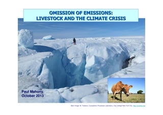
1. OMISSION OF EMISSIONS:
LIVESTOCK AND THE CLIMATE CRISIS
Paul Mahony
October 2013
Main Image: M. Todesco, Cryospheric Processes Laboratory, City College New York City, http://cryocity.org/

2. Presentation outline
Our warming planet
The Arctic “big melt”
Extreme weather events
Livestock:
Inherent inefficiency
Inte
r-
rela
ted
Scale
Greenhouse gases and other warming agents
Land clearing and degradation
Paul Mahony 2013
Nutrition
Conclusion: This is an emergency!

3. For more information
terrastendo.net

4. Paul Mahony 2013
Our warming planet
http://www.nasa.gov/multimedia/videogallery/index.html?media_id=123437001
4

5. Paul Mahony 2013
Our warming planet
http://www.nasa.gov/multimedia/videogallery/index.html?media_id=123437001
5

6. Paul Mahony 2013
Our warming planet
http://www.nasa.gov/multimedia/videogallery/index.html?media_id=123437001
6

7. Paul Mahony 2013
Our warming planet
NASA Goddard Institute for Space Studies Surface Temperature Analysis, http://data.giss.nasa.gov/cgibin/gistemp/do_nmap.py?year_last=2012&month_last=1&sat=4&sst=1&type=anoms&mean_gen=11&year1=2010&year2=2010&b
ase1=1951&base2=1980&radius=1200&pol=reg
7

8. Our warming planet
300
1750
2,000 years
Paul Mahony 2013
Atmospheric concentrations of CO2
Source: Adapted from CSIRO, “The Science of Climate Change: Questions and Answers”,
8
Fig. 4.1, p. 10
0

9. Our warming planet
393 ppm as
at Sep 2013
2000
380
300
1750
2,000 years
Paul Mahony 2013
Atmospheric concentrations of CO2
Source: Adapted from CSIRO, “The Science of Climate Change: Questions and Answers”,
9
Fig. 4.1, p. 10
0

10. GHGs, sea levels and temperature
Potentially
catastrophic
Paul Mahony 2013
Benign
Note: The shaded circle includes the 10,000 years (approx.) of human
civilisation.
Source: Hansen, J. et al “Target Atmospheric CO2: Where Should Humanity Aim?”, 2008
http://pubs.giss.nasa.gov/abstracts/2008/Hansen_etal.html
10

11. The Arctic “Big Melt”
Paul Mahony 2013
1984
NASA Earth Observatory, http://earthobservatory.nasa.gov/IOTD/view.php?id=79256&src=eorss-iotd
11

12. The Arctic “Big Melt”
Paul Mahony 2013
2012
1984
NASA Earth Observatory, http://earthobservatory.nasa.gov/IOTD/view.php?id=79256&src=eorss-iotd
12

13. The Arctic “Big Melt”
Paul Mahony 2013
Equivalent to (next slide)
Walt Meier, National Snow and Ice Data Center, “Record Low Arctic Sea Ice Extent in 2012: An exclamation point on a long-term declining trend”
http://www.nws.noaa.gov/om/csd/content/seminars/semser_20120912_meier_walt/semser_20120912_meier_walt_1.pdf (Slide 8)
13

14. The Arctic “Big Melt”
Paul Mahony 2013
Equivalent to:
Walt Meier, National Snow and Ice Data Center, “Record Low Arctic Sea Ice Extent in 2012: An exclamation point on a long-term declining trend”
http://www.nws.noaa.gov/om/csd/content/seminars/semser_20120912_meier_walt/semser_20120912_meier_walt_1.pdf (Slide 8)
14

15. Paul Mahony 2013
The Arctic “Big Melt”
National Snow & Ice Data Center, September 2012 compared to previous years, http://nsidc.org/arcticseaicenews/2012/10/poles-apart-a-recordbreaking-summer-and-winter/
15

16. Paul Mahony 2013
The Arctic “Big Melt”
National Snow & Ice Data Center, September 2012 compared to previous years, http://nsidc.org/arcticseaicenews/2012/10/poles-apart-a-recordbreaking-summer-and-winter/
16

17. Paul Mahony 2013
The Arctic “Big Melt”
From Brook, B. “Depressing climate-related trends – but who gets it?”, 6 Nov 2011
http://bravenewclimate.com/2011/11/06/depressing-climate-trends/ based on Pan-Arctic Ice Ocean Modeling and Assimilation System
(PIOMAS, Zhang and Rothrock, 2003) graphs from the Polar Science Center of the Applied Physics Laboratory at the University of
17
Washington, http://psc.apl.washington.edu/wordpress/research/projects/arctic-sea-ice-volume-anomaly/, reported in
http://neven1.typepad.com/blog/2011/10/piomas-september-2011-volume-record-lower-still.html

18. The Arctic “Big Melt”
16.9
Volume (area and thickness)
Paul Mahony 2013
3.6
Chart by L. Hamilton, based on Pan-Arctic Ice Ocean Modeling and Assimilation System (PIOMAS) data from the Polar Science Center
http://psc.apl.washington.edu/wordpress/research/projects/arctic-sea-ice-volume-anomaly/, cited in Romm, J, “Experts Warn Of ‘Near
Ice-Free Arctic In Summer’ In A Decade”, 6 September, 2012, The Energy Collective,
http://theenergycollective.com/josephromm/110216/death-spiral-watch-experts-warn-near-ice-free-arctic-summer-decade-if-volumetrend
18

19. Paul Mahony 2013
The Arctic “Big Melt”
http://www.nasa.gov/topics/earth/features/greenland-melt.html
"Greenland Melting Breaks Record Four Weeks Before Season's End", ScienceDaily, 15 August, 2012,
http://www.sciencedaily.com/releases/2012/08/120815121318.htm
19

20. The Arctic “Big Melt”
Paul Mahony 2013
ne
ergo lly
nd
had u amatica by
t
shee had dr
ed
e
thaw
nd ic elting
nla
had
Gree ys, the m surface
he
t
t of t few da
shee
en
a
ice
erc
40 p e. In just nt of the
out
2, ab e surfac 97 perce
01
uly 2 near th mated
J
i
On 8 g at or
n est
in
da
thaw rated an
le
acce 2.
1
July
http://www.nasa.gov/topics/earth/features/greenland-melt.html
"Greenland Melting Breaks Record Four Weeks Before Season's End", ScienceDaily, 15 August, 2012,
http://www.sciencedaily.com/releases/2012/08/120815121318.htm
20

21. Paul Mahony 2013
Greenland Ice Sheet
Scale comparison of Greenland (the largest island) and Australia (the smallest continent) by Joanna Serah, 26 Oct
2011, http://en.wikipedia.org/wiki/File:Australia-Greenland_Overlay.png
21

22. Paul Mahony 2013
Greenland Ice Sheet
M. Todesco, Cryospheric Processes Laboratory, City College New York City, http://cryocity.org/
22

23. Greenland Ice Sheet
Paul Mahony 2013
st
wide or
its
ss at onsible f
cro
km a be resp
00
g, 11 e would
n
km lo earanc
400
ost 2 al disapp
lm
t is a . Its tot
hee
ice s km thick .
d
rise
enlan than 2
Gr e
evel
e
or
al
The
nd m tres of se
a
point 7 me
nd
arou
M. Todesco, Cryospheric Processes Laboratory, City College New York City, http://cryocity.org/
23

24. Greenland Ice Sheet
Graphic video of Greenland torrents cascading down a moulin or crater
to the base: http://www.youtube.com/watch?v=lGxLs8YV9MM
Paul Mahony 2013
As of 2009, the Greenland ice sheet was losing over 250 cubic
kilometres of ice per year in a dynamic wet melting process, after
neither gaining nor losing mass at a substantial rate as recently as the
1990’s.
This dynamic melting process is not taken into account in the IPCC’s
projections of sea level rise. (Refer to subsequent slides.)
Video: M. Todesco, Cryospheric Processes Laboratory, City College New York City, http://cryocity.org/
Comments on loss of ice mass: Hansen, J., “Storms of my grandchildren”, Bloomsbury, pp. 255-256 and p. 287. (An
alternative ice loss figure to the quoted figure of 250 cubic km from p. 287 had been shown on p. 255 but the correct
figure has been confirmed as 250 cubic km in emails of 15th and 16th June, 2011.)
24

25. Greenland Ice Sheet
If the annual water flows were poured over Germany . . .
Based on ice mass loss
of 250 cubic km per
annum
Paul Mahony 2013
0.71 metres
25

26. Paul Mahony 2013
All Ice Sheets and Glaciers
NSIDC, “The Contribution of the Cryosphere to Changes in Sea Level”, http://nsidc.org/cryosphere/sotc/sea_level.html
26

27. Paul Mahony 2013
All Ice Sheets and Glaciers
NSIDC, “The Contribution of the Cryosphere to Changes in Sea Level”, http://nsidc.org/cryosphere/sotc/sea_level.html
27

28. Global sea level rise
Projections to 2100:
IPCC:
Up to 1 metre (but higher values cannot be
excluded)
Vermeer and Rahmstorf: nearly 2 metres
Hansen:
Likely several metres (see next slide) if we
continue with “business as usual”, depending
on impact of negative (diminishing) feedbacks.
Impacts:
Experienced through “high sea-level events” .
Paul Mahony 2013
A combination of sea-level rise, high tide and storm surge.
Increased likelihood with 0.5 of a metre: 100 to 1,000 fold increase
Steffen, W, “The Critical Decade: Climate Science, risks and responses”, Climate Commission, Fig. 8, p. 12
http://climatecommission.gov.au/topics/the-critical-decade/
Spratt, D, “NASA climate chief demolishes denialist claims on sea levels”, 26 Oct 2012, http://www.climatecodered.org/2012/10/nasa-climate- 28
chief-demolishes-denialist.html and Hansen, J & Sato, M “Update of Greenland Ice Sheet Mass Loss: Exponential?”, 26 Dec 2012

29. Global sea level rise
What about IPCC’s projection of less than 1 metre?
Only allows for certain short feedback mechanisms, e.g. changes in:
• water vapour
• clouds
• sea ice
Does not allow for slow feedbacks, e.g.:
• ice sheet dynamics;
• changes in vegetation cover;
Paul Mahony 2013
• permafrost melting; and
• carbon-cycle feedbacks.
Spratt, D and Sutton, P, “Climate Code Red: The case for emergency action”, Scribe, 2008, p. 47
29

30. Permafrost
• Dramatic and unprecedented plumes of methane . . .
have been seen bubbling to the surface of the Arctic
Ocean by scientists undertaking an extensive survey of
the region.
Paul Mahony 2013
• The scale and volume of the methane release has
astonished the head of the Russian research team
who has been surveying the seabed of the east
Siberian Arctic Shelf off northern Russia for nearly 20
years.
• Igor Semiletov of the International Arctic Research
Centre at the University of Alaska Fairbanks . . . said
that he has never before witnessed the scale and force
has never before witnessed the scale and force
of the methane being released from beneath the Arctic
seabed.
Connor, S, “Vast methane 'plumes' seen in Arctic ocean as sea ice retreats”, The Independent, 13 December,
2011, http://www.independent.co.uk/news/science/vast-methane-plumes-seen-in-arctic-ocean-as-sea-ice-retreats30
6276278.html (Accessed 4 February 2012)

31. Permafrost
Dramatic and unprecedented
Paul Mahony 2013
astonished
has never before witnessed the scale and force
of the methane being released from beneath the Arctic
seabed.
Connor, S, “Vast methane 'plumes' seen in Arctic ocean as sea ice retreats”, The Independent, 13 December,
2011, http://www.independent.co.uk/news/science/vast-methane-plumes-seen-in-arctic-ocean-as-sea-ice-retreats31
6276278.html (Accessed 4 February 2012)

32. Paul Mahony 2013
Extreme Weather
Australian Climate Commission: “The Angry Summer”, http://pandora.nla.gov.au/pan/136923/201309191415/climatecommission.gov.au/report/the-angry-summer/index.html
32

33. Livestock
Inherent inefficiency
Inte
r-
rela
ted
Scale
Greenhouse gases and other warming agents
Paul Mahony 2013
Land clearing and degradation

34. Livestock
Emissions omitted because relevant factors are:
(a) omitted entirely from official figures, e.g.
tropospheric ozone and foregone sequestration
(b) classified under different headings, e.g. livestockrelated land clearing reported under “land use,
land use change and forestry”
Paul Mahony 2013
(c) considered but with conservative calculations, e.g.
methane’s impact based on a 100-year, rather than
20-year, “global warming potential”

35. Paul Mahony 2013
Inherent inefficiencies
Derived from W.O. Herring and J.K. Bertrand, “Multi-trait Prediction of Feed
Conversion in Feedlot Cattle”, Proceedings from the 34th Annual Beef
Improvement Federation Annual Meeting, Omaha, NE, July 10-13, 2002,
www.bifconference.com/bif2002/BIFsymposium_pdfs/Herring_02BIF.pdf, cited
in Singer, P & Mason, J, “The Ethics of What We Eat” (2006), Text Publishing
Company, p. 210

36. Paul Mahony 2013
Inherent inefficiencies
Derived from W.O. Herring and J.K. Bertrand, “Multi-trait Prediction of Feed
Conversion in Feedlot Cattle”, Proceedings from the 34th Annual Beef
Improvement Federation Annual Meeting, Omaha, NE, July 10-13, 2002,
www.bifconference.com/bif2002/BIFsymposium_pdfs/Herring_02BIF.pdf, cited
in Singer, P & Mason, J, “The Ethics of What We Eat” (2006), Text Publishing
Company, p. 210

37. Inherent inefficiencies
)PPN ro ytivitcudorp yramirp ten( htworg
tnalp launna s’htraE fo noitairporppA
Other
30%
Livestock
58%
Paul Mahony 2013
Humans
12%
Sources: Derived from Fridolin Krausmann, et al “Global patterns of socioeconomic biomass flows in the year 2000: A
comprehensive assessment of supply, consumption and constraints” and Helmut Haberl, et al “Quantifying and
mapping the human appropriation of net primary production in earth's terrestrial ecosystems”, cited in Russell, G.
“Burning the biosphere, boverty blues (Part 1)”, www.bravenewclimate.com

38. Inherent inefficiencies
ekatni eirolac ’snamuH
)PPN ro ytivitcudorp yramirp ten( htworg
tnalp launna s’htraE fo noitairporppA
Other
30%
17%
Livestock
58%
83%
Paul Mahony 2013
Humans
12%
Sources: Derived from Fridolin Krausmann, et al “Global patterns of socioeconomic biomass flows in the year 2000: A
comprehensive assessment of supply, consumption and constraints” and Helmut Haberl, et al “Quantifying and
mapping the human appropriation of net primary production in earth's terrestrial ecosystems”, cited in Russell, G.
“Burning the biosphere, boverty blues (Part 1)”, www.bravenewclimate.com

39. Inherent inefficiencies
• At present, the US livestock population consumes more
than 7 times as much grain as is consumed directly by the
entire American population.
Paul Mahony 2013
US Department of Agriculture, 2001. Agricultural statistics, Washington, DC
The above reference was cited in Pimentel, D. & Pimentel M. “Sustainability of meat-based and plant-based
diets and the environment”, American Journal of Clinical Nutrition, Vol. 78, No. 3, 660S-663S, September
2003

40. Inherent inefficiencies
• The amount of grains fed to US livestock is sufficient to feed
about 840 million people who follow a plant-based diet
Dr David Pimentel, Cornell University “Livestock production and energy
use”, Cleveland CJ, ed. Encyclopedia of energy (in press). [Cited 2003]
• Existing Cropland Could Feed 4 Billion More (incl. US
cropland 1 billion more)
University of Minnesota, 2013
Paul Mahony 2013
Pimentel, D. & Pimentel M. “Sustainability of meat-based and plant-based diets and the environment”,
American Journal of Clinical Nutrition, Vol. 78, No. 3, 660S-663S, September 2003
Emily S Cassidy, Paul C West, James S Gerber and Jonathan A Foley, “Redefining agricultural yields: from
tonnes to people nourished per hectare”, http://iopscience.iop.org/1748-9326/8/3/034015 and
http://www1.umn.edu/news/news-releases/2013/UR_CONTENT_451697.html

41. Scale
“In the United States, more than 9 billion livestock are
maintained to supply the animal protein consumed
each year.”
Paul Mahony 2013
US Department of Agriculture, Agricultural statistics, 2001
The above reference was cited in Pimentel, D. & Pimentel M. “Sustainability of meat-based and plant-based
diets and the environment”, American Journal of Clinical Nutrition, Vol. 78, No. 3, 660S-663S, September
2003

42. Scale
Cattle, sheep and goat population in 2006 3.3 billion:
3,600
3,400
M illio n In d iv id u a ls
3,200
3,000
2,800
2,600
2,400
2,200
2,000
1960
1970
1980
1990
2000
2010
Source: FAO; UNPop
Land animals slaughtered 2011: 64 billion approx. incl. over 58 billion
chickens globally and 550 million chickens in Australia
• Plus laying hens
6.5 billion
• Plus milk providers 0.7 billion
Livestock biomass 700m tonnes v. human biomass 335m tonnes.
Paul Mahony 2013
Livestock/wildlife ratio 23:3
Source: Chart - UN FAO cited in Earth Policy Institute book_wote_ch3_13.xls, http://www.earth-policy.org
Slaughter numbers: FAO STAT http://faostat.fao.org/site/569/default.aspx#ancor
Laying hens & milk providers – FAOSTAT, http://faostat.fao.org/site/291/default.aspx,
Biomass – Geoff Russell “Burning the biosphere – Boverty Blues Pt. 1”, www.bravenewclimate.com
Livestock/wildlife ratio – UN Food & Agriculture Organization “Livestock’s Long Shadow”, 2006

43. Some context for beef: Aluminium
Paul Mahony 2013
Based on conservative 100 year GWP
43

44. Some context for beef: Aluminium
Based on conservative 100 year GWP
16% of Australia’s electricity
but provides only 0.06% of jobs
and 0.23% of GDP.
Paul Mahony 2013
2.5 times the world average of
GHGs per tonne of product.
Sources: Hamilton, C, “Scorcher: The Dirty Politics of Climate Change”, (2007) Black Inc Agenda, p. 40; Turton, H. “The Aluminium
Smelting Industry Structure, market power, subsidies and greenhouse gas emissions”, The Australia Institute, Discussion Paper
Number 44, January 2002, ISSN 1322-5421, p. ix; Turton, H. “Greenhouse gas emissions in industrialised countries Where does
Australia stand?”, The Australia Institute, Discussion Paper Number 66, June 2004, ISSN 1322-5421, p. viii.
44

45. Paul Mahony 2013
So how does beef compare?
45

46. Based on conservative 100 year GWP
GHG Emissions Intensity (kg of GHG per kg of product)
60
50
40
30
20
10
0
Paul Mahony 2013
Wheat
Other
grains
Sugar
Cement,
lime, etc
Steel

47. Based on conservative 100 year GWP
GHG Emissions Intensity (kg of GHG per kg of product)
60
50
40
30
20
10
0
Paul Mahony 2013
Wheat
Other
grains
Sugar
Cement,
lime, etc
Steel
Aluminium

48. Based on conservative 100 year GWP
GHG Emissions Intensity (kg of GHG per kg of product)
60
50
40
30
20
10
0
Paul Mahony 2013
Wheat
Other
grains
Sugar
Cement,
lime, etc
Steel
Alumin- Other nonferrous
ium

49. Based on conservative 100 year GWP
GHG Emissions Intensity (kg of GHG per kg of product)
60
50
40
30
20
10
0
Paul Mahony 2013
Wheat
Other
grains
Sugar
Cement,
lime, etc
Steel
Alumin- Other nonferrous
ium
Wool

50. Based on conservative 100 year GWP
GHG Emissions Intensity (kg of GHG per kg of product)
60
50
40
30
20
10
0
Paul Mahony 2013
Wheat
Other
grains
Sugar
Cement,
lime, etc
Steel
Alumin- Other nonferrous
ium
Wool
Sheep
meat

51. Based on conservative 100 year GWP
GHG Emissions Intensity (kg of GHG per kg of product)
60
50
40
30
20
10
0
Paul Mahony 2013
Wheat
Other
grains
Sugar
Cement,
lime, etc
Steel
George Wilkenfeld & Associates Pty Ltd and Energy Strategies,
National Greenhouse Gas Inventory 1990, 1995, 1999, End Use
Allocation of Emissions Report to the Australian Greenhouse
Office, 2003, Volume 1, Table S5, p. vii
Alumin- Other nonferrous
ium
Wool
Sheep
meat
Beef

52. Based on conservative 100 year GWP
GHG Emissions Intensity (kg of GHG per kg of product)
60
e
of th
55%
und the time
aro
50
only duct at
As
pro
ght.
end
wei
ss
the
carca ensity of
n
40
sed o ions int
ba
ss
iss
was
g.
arca t
em
kg
nc
3k
of 51 meat, the around 9
sed o imes tha
re
ba
30
8 kg ound 5 t
s figu sed as
een
’
b
67.
Beef s is u
have
lly is duct (ar
s
ba
uld
carca rting wo
ty glo end pro
si
20 repo
inten for the
of
ions
miss d 123 kg
e
eef’s aroun
:B
2013 uates to
10
AO
UN F t. That eq minium).
h
u
weig tralian al
s
0
of Au
Paul Mahony 2013
Wheat
Other
grains
Sugar
Cement,
lime, etc
Steel
Alumin- Other nonferrous
ium
Wool
Sheep
meat
Beef
1. George Wilkenfeld & Associates Pty Ltd and Energy Strategies, National Greenhouse Gas Inventory 1990, 1995, 1999, End
Use Allocation of Emissions Report to the Australian Greenhouse Office, 2003, Volume 1, Table S5, p. vii
2. Opio, C., Gerber, P., Mottet, A., Falcucci, A., Tempio, G., MacLeod, M., Vellinga, T., Henderson, B. & Steinfeld, H. 2013.
Greenhouse gas emissions from ruminant supply chains - A global life cycle assessment. Food and Agriculture Organization of
the United Nations (FAO), Rome, http://www.fao.org/docrep/018/i3461e/i3461e.pdf

53. Based on conservative 100 year GWP
GHG Emissions Intensity (kg of GHG per kg of product)
60
50
40
Remember, this chart is
about emissions intensity.
30
20
Things get even worse
when you realise that we
produce 10% more beef
than aluminium.
10
0
Paul Mahony 2013
Wheat
Other
grains
Sugar
Cement,
lime, etc
Steel
George Wilkenfeld & Associates Pty Ltd and Energy Strategies,
National Greenhouse Gas Inventory 1990, 1995, 1999, End Use
Allocation of Emissions Report to the Australian Greenhouse
Office, 2003, Volume 1, Table S5, p. vii
Alumin- Other nonferrous
ium
Wool
Sheep
meat
Beef

54. Based on conservative 100 year GWP
Paul Mahony 2013
GHG Emissions - Absolute
George Wilkenfeld & Associates Pty Ltd and Energy Strategies, National Greenhouse Gas Inventory 1990, 1995, 1999,
End Use Allocation of Emissions Report to the Australian Greenhouse Office, 2003, Volume 1, Table S5, p. vii
54

55. Based on conservative 100 year GWP
Emissions Intensity: A Swedish Study
35
kg CO2-e per kg of product
30
25
20
15
10
5
Paul Mahony 2013
0
Carrots: domestic, fresh
Honey
Apples: fresh, overseas by boat
Milk: domestic, 4% fat
Italian pasta: cooked
Rice: cooked
Herring: domestic, cooked
Eggs: Swedish, cooked
Chicken: fresh, domestic, cooked
Pork: domestic, fresh, cooked
Tropical fruit: fresh, overseas by plane
Potatoes: cooked, domestic
Whole wheat: domestic, cooked
Soybeans: cooked, overseas by boat
Sugar: domestic
Oranges: fresh, overseas by boat
Green beans: South Europe, boiled
Vegetables: frozen, overseas by boat, boiled
Rapeseed oil: from Europe
Cod: domestic, cooked
Cheese: domestic
Beef: domestic, fresh, cooked
Carlsson-Kanyama, A. & Gonzalez, A.D. “Potential Contributions of Food Consumption Patterns to Climate Change”, The
American Journal of Clinical Nutrition, Vol. 89, No. 5, pp. 1704S-1709S, May 2009,
http://www.ajcn.org/cgi/content/abstract/89/5/1704S
55

56. CO2-e equivalent (CO2-e) emissions from livestock
20-year “Global Warming Potential” (GWP)
Traditional reporting of
methane’s global warming
potential has understated its
shorter-term impact, as it breaks
down in the atmosphere much
faster than carbon dioxide.
The IPCC’s 100-year GWP for
methane was 25 in 2007 but has
been increased to 34 (with
carbon cycle feedbacks) in 2013.
The corresponding figures for a
100 year timeframe are 72 and
86.
Paul Mahony 2013
NASA reports figures of 33 for
100 years and 105 for 20 years.
Chart: Smith, K., cited in World Preservation Foundation, “Reducing Shorter-Lived Climate Forcers through Dietary Change: Our
best chance for preserving global food security and protecting nations vulnerable to climate change“,
http://www.worldpreservationfoundation.org/Downloads/ReducingShorterLivedClimateForcersThroughDietaryChange.pdf
Romm, J. “More Bad News For Fracking: IPCC Warns Methane Traps Much More Heat Than We Thought”, Climate Progress, 2
Oct 2013, http://thinkprogress.org/climate/2013/10/02/2708911/fracking-ipcc-methane/
Sanderson, K., “Aerosols make methane more potent”, Nature, Published online 29 October 2009 | Nature |
doi:10.1038/news.2009.1049, http://www.nature.com/news/2009/091029/full/news.2009.1049.html
56

57. CO2-e emissions from Australian livestock
59 mt
approx.
The official Australian figure of 59mt represents 10.7% of Australia’s
total emissions of 549mt.
It is based solely on enteric fermentation and manure management.
Adding emissions from livestock-related deforestation and savannaburning increases livestock’s emissions to 106mt or 17.8% of the
revised total.
Paul Mahony 2013
Using a 20-year GWP, the final percentage increases to 30.5%.
Source:
- Dept of Climate Change & Energy Efficiency, National Greenhouse Inventory 2008, Fig. 15, p. 15
- Livestock’s share of deforestation and savanna burning derived from George Wilkenfeld & Associates
57
Pty Ltd and Energy Strategies, National Greenhouse Gas Inventory 1990, 1995, 1999, End Use
Allocation of Emissions Report to the Australian Greenhouse Office, 2003

58. CO2-e emissions from Australian livestock
Based on conservative 100 year GWP
If we were to consider end-use, the percentage would be 30.64%.
30.64%
Animal Agriculture
Other
Paul Mahony 2013
69.36%
Source: The University of Sydney and CSIRO, 2005, “Balancing Act – A Triple Bottom Line
Analysis of the Australian Economy”
58

59. CO2-e emissions from livestock globally
18%
Animal Agriculture
Other
82%
49%
Animal Agriculture
51.00%
43%
Other
Animal Agriculture
Other
Paul Mahony 2013
57%
World Watch Institute, 2009 (amended)
- As above but amended (by this presenter)
by removing livestock respiration as a factor
United Nations Food & Agriculture Organization,
“Livestock’s Long Shadow”, 2006
- Significantly more than all the world’s transport
- Excludes factors considered by the World Watch
Institute (refer below)
- Amended to 14.5% in 2013 (See slide 51 of this
presentation and full report at
http://www.fao.org/docrep/018/i3461e/i3461e.pdf).
World Watch Institute, 2009
- 20 year GWP on methane
- Foregone sequestration on land previously cleared*
- Livestock respiration overwhelming photosynthesis in
absorbing carbon
- Increased livestock production since 2002
- Corrections in documented under-counting
- More up to date emissions figures
- Corrections for use of Minnesota for source data
- Re-alignment of sectoral information
- Fluorocarbons for extended refrigeration
- Cooking at higher temperature and for longer periods
- Disposal of waste
- Production, distribution and disposal of by-products and
packaging
- Carbon-intensive medical treatment of livestock-related
illness
* Foregone sequestration still not fully accounted for.
Source of World Watch material: Goodland, R & Anhang, J, “Livestock and Climate Change - What if the key actors in climate change are 59
cows, pigs, and chickens?”, World Watch, Nov/Dec, 2009, pp 10-19. (Note: Robert Goodland was formerly lead environmental adviser at the
World Bank. Jeff Anhang is a research officer and environmental specialist at the World Bank Group’s International Finance Corporation.)

60. Paul Mahony 2013
Land Clearing
60

61. Land Clearing in Australia
Total area cleared since European settlement approx. 1 million sq. km.
Approx. 70% or 700,000 sq km (9% of Australia’s land area) is due to livestock.
Cleared native vegetation and protected areas
Cleared native vegetation
Native vegetation
Paul Mahony 2013
Protected areas
Sources: Map - National Biodiversity Strategy Review Task Group, “Australia’s
Biodiversity Conservation Strategy 2010–2020”, Figure A10.1, p. 91
Other figures derived from Russell, G. “The global food system and climate
change – Part 1”, 9 Oct 2008, www.bravenewclimate.com, which utilised:
Dept. of Sustainability, Environment, Water, Population and Communities,
State of the Environment Report 2006, Indicator: LD-01 The proportion and
area of native vegetation and changes over time, March 2009; and
ABS, 4613.0 “Australia’s Environment: Issues and Trends”, Jan 2010; and
ABS 1301.0 Australian Year Book 2008, since updated for 2009-10, 16.13 Area of crops
61

62. Rainforest destruction in Africa
Paul Mahony 2013
The vertical lines primarily
represent the Guinea Savanna,
which was once forest and is
maintained as savanna through
regular burning, primarily to
enable cattle grazing.
Sources: Mahesh Sankaran, et al, “Determinants of woody cover in African savannas”, Nature 438, 846-849 (8 December
2005), cited in Russell, G. “Burning the biosphere, boverty blues (Part 2)”, www.bravenewclimate.com
62

63. Paul Mahony 2013
Rainforest destruction in Africa
Sources: Mahesh Sankaran, et al, “Determinants of woody cover in African savannas”, Nature 438, 846-849 (8 December
2005), cited in Russell, G. “Burning the biosphere, boverty blues (Part 2)”, www.bravenewclimate.com
MODIS Rapid Response Team, NASA Goddard Space Flight Center, http://rapidfire.sci.gsfc.nasa.gov/firemaps/
63

64. Paul Mahony 2013
Rainforest destruction in Africa
Sources: Mahesh Sankaran, et al, “Determinants of woody cover in African savannas”, Nature 438, 846-849 (8 December
2005), cited in Russell, G. “Burning the biosphere, boverty blues (Part 2)”, www.bravenewclimate.com
MODIS Rapid Response Team, NASA Goddard Space Flight Center, http://rapidfire.sci.gsfc.nasa.gov/firemaps/
64

65. Rainforest destruction in South America
Winds transport black carbon
from the Amazon to the Antarctic
Peninsula.
47% to 61% of black carbon in
Antarctica comes from pasture
management in the Amazon and
Africa.
Black carbon melts ice rapidly by
absorbing heat from sunlight.
Paul Mahony 2013
http://www.world-maps.co.uk/continent-map-of-south-america.htm
http://rainforests.mongabay.com/amazon/amazon_map.html
MODIS Rapid Response Team, NASA Goddard Space Flight
Center - http://rapidfire.sci.gsfc.nasa.gov/firemaps/
Black carbon information: Presentation by Gerard Bisshop, World Preservation Fund presentation to Cancun Climate
Summit, Dec, 2010 “Shorter lived climate forcers: Agriculture Sector and Land Clearing for Livestock” (co-authors
Lefkothea Pavlidis and Dr Hsien Hui Khoo). MODIS Rapid Response Team, NASA Goddard Space Flight Center http://rapidfire.sci.gsfc.nasa.gov/firemaps/
65

66. Paul Mahony 2013
Burning in Australia
To put Australian savanna burning into context, the 2009 Black Saturday bushfires in the state of
Victoria burnt around 4,500 hectares. In comparison, each year in northern Australia where 70% of
our cattle graze, we burn 100 times that area across the tropical savanna.
Source: Modis fire map, NASA
66

67. Land clearing in Australia
Paul Mahony 2013
of
ddle
i
the m
om
ast fr
ge
d
unnin etation.
nslan
ne r veg
li
ee
i n Qu
10 km ooded
ed
fa
clear
er w
rth o
as
no
oth
as w
land rest and
the
and
that ed by fo
uch l
m
ed
ar as
ssum as cover
a
cle
If we urne w
o to
eg
elbo
ul d w ?
M
wo
orth nd 2008
rn
ow fa 1988 a
H
n
twee
be
10 km
Original Map: Copyright 2010 Melway Publishing Pty Ltd. Reproduced from Melway Edition 38 with permission.
67

68. Land clearing in Australia
Paul Mahony 2013
10 km
Original Map: Copyright 2010 Melway Publishing Pty Ltd. Reproduced from Melway Edition 38 with permission.
68

69. Land clearing in Australia – Queensland 1988 -2008
Approximately 78,000 square kilometres
Paul Mahony 2013
Cairns
Source:
Derived from Bisshop, G. & Pavlidis, L, “Deforestation and land
degradation in Queensland - The culprit”, Article 5, 16th Biennial Australian
Association for Environmental Education Conference, Australian National
University, Canberra,
26-30 September 2010
Original map: www.street-directory.com.au. Used with permission.
(Cairns inserted by this presenter.)
69

70. Land clearing in Australia – Queensland 1988 -2008
Approximately 78,000 square kilometres
Cairns
Paul Mahony 2013
sq
,000
78
km
Source:
Derived from Bisshop, G. & Pavlidis, L, “Deforestation and land
degradation in Queensland - The culprit”, Article 5, 16th Biennial Australian
Association for Environmental Education Conference, Australian National
University, Canberra,
26-30 September 2010
Original map: www.street-directory.com.au. Used with permission.
(Cairns inserted by this presenter.)
70

71. Land clearing
UN Food & Agriculture Organization:
“Directly and indirectly, through grazing and through feedcrop production, the
livestock sector occupies about 30 percent ice-free terrestrial surface of the
planet.”
Paul Mahony 2013
PBL Netherlands Environmental Assessment Agency:
“ . . . a global food transition to less meat, or even a complete switch to plantbased protein food [was found] to have a dramatic effect on land use. Up to
2,700 Mha of pasture and 100 Mha of cropland could be abandoned, resulting
in a large carbon uptake from regrowing vegetation. Additionally, methane
and nitrous oxide emissions would be reduced substantially.” A plant-based
diet would reduce climate change mitigation costs by 80%. A meat-free diet
would reduce them by 70%.
Zero Carbon Britain:
“ZCB 2030 will revolutionise our landscape and diets. An 80% reduction in
meat and dairy production will free up land to grow our own food and fuel
whilst also sequestering carbon from the atmosphere.”
Steinfeld, H. et al. 2006, “Livestock’s Long Shadow: Environmental Issues and Options. Livestock, Environment and Development“, FAO, Rome, p. 4.
Elke Stehfest, Lex Bouwman, Detlef P. van Vuuren, Michel G. J. den Elzen, Bas Eickhout and Pavel Kabat, “Climate benefits of changing diet” Climatic
Change, Volume 95, Numbers 1-2 (2009), 83-102, DOI: 10.1007/s10584-008-9534-6 (Also http://www.springerlink.com/content/053gx71816jq2648/)
Centre for Alternative Technology, Wales, “Zero Carbon Britain”, 2010, http://www.zerocarbonbritain.com/ and
http://www.zerocarbonbritain.com/resources/factsheets
71

72. Bill McKibben 350.org
McKibben’s position does not stand up to close scrutiny, and can be
paraphrased as:
Paul Mahony 2013
“If we want to reduce emissions from animal agriculture, we need to
move away from factory farming, adopt a modified form of grazing,
and buy locally.”
See “Do the math: there are too many cows”
and
“Livestock and climate: Why Alan Savory is not a saviour”
http://terrastendo.net/2013/07/26/do-the-math-there-are-too-many-cows/
http://terrastendo.net/2013/03/26/livestock-and-climate-why-allan-savory-is-not-a-saviour/
72

73. Bill McKibben 350.org
Paul Mahony 2013
Livestock population
McKibben’s suggestion that there were “big herds of big animals” before European settlement
is difficult to reconcile with the fact that the native pronghorn (the USA’s “antelope”) generally
weigh around one-tenth as much as cows and bulls bred for beef. Even allowing for bison, the
biomass of native animals was significantly less than that of modern day livestock.
73

74. Bill McKibben 350.org
Paul Mahony 2013
Livestock population
Russel, G. “Forget the quality, it’s the 700 million tonnes which counts“, 17 Nov 2009,
http://bravenewclimate.com/2009/11/17/700-million-from-livestock/, citing Subak, S., “GEC-1994-06 : Methane from the House
of Tudor and the Ming Dynasty“, CSERGE Working Paper, http://www.cserge.ac.uk/sites/default/files/gec_1994_06.pdf and
Thorpe, A. “Enteric fermentation and ruminant eructation: the role (and control?) of methane in the climate change debate“,
Climatic Change, April 2009, Volume 93, Issue 3-4, pp 407-431, http://link.springer.com/article/10.1007%2Fs10584-008-9506-x
74

75. Livestock
Bill McKibben 350.org
Paul Mahony 2013
Despite what McKibben says, buying Locally doesn’t help much
Soy transport figure used here, as beef’s was not specified in the relevant study. In this
case, unlike soy, there appears to be no sea transport involved in the beef emissions figure.
In the absence of a more precise figure, we have assumed that beef’s transport-related
emissions per kilogram of product are the same as those of soy, even though they are likely
to be less.
Carlsson-Kanyama, A. & Gonzalez, A.D. “Potential Contributions of Food Consumption Patterns to Climate Change”, The
American Journal of Clinical Nutrition, Vol. 89, No. 5, pp. 1704S-1709S, May 2009,
http://www.ajcn.org/cgi/content/abstract/89/5/1704S
75

76. Paul Mahony 2013
James Hansen – Essential Measures
James Hansen, former Director of the Goddard Institute for Space Studies, NASA

77. James Hansen – Essential Measures
1. End coal-fired power.
2. Massive reforestation.
Required to reduce CO2
concentrations to < 350
ppm (currently 390 ppm
approx.)
A key factor in reducing CO2 concentrations will be
measure 2.
Not possible without
addressing animal agriculture.
Paul Mahony 2013
Hansen also discusses the importance of non-CO2 forcings.
They include methane, nitrous oxide, tropospheric ozone and
black carbon. Animal agriculture is a key contributor.
Source: Hansen, J; Sato, M; Kharecha, P; Beerling, D; Berner, R; Masson-Delmotte, V; Pagani, M; Raymo, M; Royer, D.L.;
and Zachos, J.C. “Target Atmospheric CO2: Where Should Humanity Aim?”, 2008.

78. Paul Mahony 2013
James Hansen – Essential Measures
Source: Hansen, J; Sato, M; Kharecha, P; Beerling, D; Berner, R; Masson-Delmotte, V; Pagani, M; Raymo, M; Royer, D.L.;
and Zachos, J.C. “Target Atmospheric CO2: Where Should Humanity Aim?”, 2008.

79. Paul Mahony 2013
Nutrition – Meat & Livestock Australia
“Five essential ingredients in one amazing food”
He’s handsome, charismatic and intelligent. Unfortunately, we’re not so
sure about Sam.

80. Protein (g) per hectare
1,200,000
Soy provides 12
times the protein of
beef per hectare . . .
1,000,000
800,000
600,000
400,000
200,000
0
Beef
Soy
Wheat
Rice
Potato
GHG per hectare
20,000
. . . for one-seventh
of the emissions.
15,000
10,000
Paul Mahony 2013
5,000
0
Beef
Soy
W heat
Rice
Potato
Source: Mahony, P, “Some Environmental Impacts of Animal Agriculture, Part 2”, updated Dec, 2010,
http://dl.dropbox.com/u/1097247/bccag/images/animals2.pdf and Mahony, P for Vegetarian Network Victoria “Submission in Response
80
to Victorian State Government’s Climate Change Green Paper”, Sep 2009,
http://www.vnv.org.au/site/files/submission090921climatechangegreenpaper.pdf

81. Protein (g) per hectare
1,200,000
Soy provides 12
times the protein of
beef per hectare . . .
1,000,000
800,000
600,000
400,000
200,000
0
Beef
Soy
Wheat
Rice
Potato
Water per hectare
20,000,000
. . . for one-third of the water.
15,000,000
10,000,000
Paul Mahony 2013
5,000,000
0
Beef
Soy
W heat
Rice
Potato
Source: Mahony, P, “Some Environmental Impacts of Animal Agriculture, Part 2”, updated Dec, 2010,
http://dl.dropbox.com/u/1097247/bccag/images/animals2.pdf and Mahony, P for Vegetarian Network Victoria “Submission in Response
81
to Victorian State Government’s Climate Change Green Paper”, Sep 2009,
http://www.vnv.org.au/site/files/submission090921climatechangegreenpaper.pdf

82. Paul Mahony 2013
30,000
0
Wheat
Lupins
Field peas
Chickpeas
Rice
Mung beans
Navy beans
Faba beans
Lentils
Barley
Oats
Maize
Sorghum
Triticale
Potatoes
Onions
Carrots
Asparagus
Broccoli
Cauliflower
Tomatoes
Mushrooms
Lettuce
Capsicum/chillies
Cabbage
Beans
Other
Soy beans
Sugar cane
Peanuts
Apples
Pears
Nashi
Avocado
Melons
Pineapples
Bananas
Kiwifruit
Mangoes
Table and dried grapes
Oranges
Mandarins
Lemons/limes/grapefruit
Peaches
Nectarines
Apricots
Plums
Cherries
Almonds
Macadamia
Berries
Beef
Lamb
Pig meat
Poultry
Whole milk
Cheese - Cheddar
Cheese - Non-Cheddar
Butter
Eggs
Tuna
Other fish
Prawns
Rock lobster
Abalone
Scallops
kcal x 1,000,000
Energy Value of food in Australia
100,000
90,000
Animal
Products
9%
80,000
70,000
60,000
50,000
40,000
Plant Products
91%
20,000
10,000
82

83. 400
0
Wheat
Lupins
Field peas
Chickpeas
Rice
Mung beans
Navy beans
Faba beans
Lentils
Barley
Oats
Maize
Sorghum
Triticale
Potatoes
Onions
Carrots
Asparagus
Broccoli
Cauliflower
Tomatoes
Mushrooms
Lettuce
Capsicum/chillies
Cabbage
Beans
Other
Soy beans
Sugar cane
Peanuts
Apples
Pears
Nashi
Avocado
Melons
Pineapples
Bananas
Kiwifruit
Mangoes
Table and dried grapes
Oranges
Mandarins
Lemons/limes/grapefruit
Peaches
Nectarines
Apricots
Plums
Cherries
Almonds
Macadamia
Berries
Beef
Lamb
Pig meat
Poultry
Whole milk
Cheese - Cheddar
Cheese - Non-Cheddar
Butter
Eggs
Tuna
Other fish
Prawns
Rock lobster
Abalone
Scallops
Oysters
Paul Mahony 2013
Tonnes
Livestock
Zinc Content
1,200
Animal Products
14%
1,000
800
600
Plant Products
86%
200
83

84. 0
Wheat
Lupins
Field peas
Chickpeas
Rice
Mung beans
Navy beans
Faba beans
Lentils
Barley
Oats
Maize
Sorghum
Triticale
Potatoes
Onions
Carrots
Asparagus
Broccoli
Cauliflower
Tomatoes
Mushrooms
Lettuce
Capsicum/chillies
Cabbage
Beans
Other
Soy beans
Sugar cane
Peanuts
Apples
Pears
Nashi
Avocado
M elons
Pineapples
Bananas
Kiwifruit
Mangoes
Table and dried grapes
Oranges
Mandarins
Lemons/limes/grapefruit
Peaches
Nectarines
Apricots
Plums
Cherries
Almonds
Macadamia
Berries
Beef
Lamb
Pig meat
Poultry
Whole milk
Cheese - Cheddar
Cheese - Non-Cheddar
Butter
Eggs
Tuna
Other fish
Prawns
Rock lobster
Abalone
Scallops
Oysters
Paul Mahony 2013
Tonnes
Livestock
Calcium Content
12,000
10,000
8,000
Animal Products
44%
Plant Products
56%
6,000
4,000
2,000
84

85. Paul Mahony 2013
0
Wheat
Lupins
Field peas
Chickpeas
Rice
Mung beans
Navy beans
Faba beans
Lentils
Barley
Oats
Maize
Sorghum
Triticale
Potatoes
Onions
Carrots
Asparagus
Broccoli
Cauliflower
Tomatoes
Mushrooms
Lettuce
Capsicum/chillies
Cabbage
Beans
Other
Soy beans
Sugar cane
Peanuts
Apples
Pears
Nashi
Avocado
Melons
Pineapples
Bananas
Kiwifruit
Mangoes
Table and dried grapes
Oranges
Mandarins
Lemons/limes/grapefruit
Peaches
Nectarines
Apricots
Plums
Cherries
Almonds
Macadamia
Berries
Beef
Lamb
Pig meat
Poultry
Whole milk
Cheese - Cheddar
Cheese - Non-Cheddar
Butter
Eggs
Tuna
Other fish
Prawns
Rock lobster
Abalone
Scallops
Oysters
Tonnes
Livestock
Protein Content
3,500,000
3,000,000
2,500,000
2,000,000
1,500,000
1,000,000
500,000
85

86. 0
Wheat
Lupins
Field peas
Chickpeas
Rice
Mung beans
Navy beans
Faba beans
Lentils
Barley
Oats
Maize
Sorghum
Triticale
Potatoes
Onions
Carrots
Asparagus
Broccoli
Cauliflower
Tomatoes
Mushrooms
Lettuce
Capsicum/chillies
Cabbage
Beans
Other
Soy beans
Sugar cane
Peanuts
Apples
Pears
Nashi
Avocado
Melons
Pineapples
Bananas
Kiwifruit
Mangoes
Table and dried grapes
Oranges
Mandarins
Lemons/limes/grapefruit
Peaches
Nectarines
Apricots
Plums
Cherries
Almonds
Macadamia
Berries
Beef
Lamb
Pig meat
Poultry
Whole milk
Cheese - Cheddar
Cheese - Non-Cheddar
Butter
Eggs
Tuna
Other fish
Prawns
Rock lobster
Abalone
Scallops
Oysters
Paul Mahony 2013
Tonnes
Livestock
Iron Content
1,600
1,400
1,200
1,000
800
600
400
200
86

87. 0
Wheat
Lupins
Field peas
Chickpeas
Rice
Mung beans
Navy beans
Faba beans
Lentils
Barley
Oats
Maize
Sorghum
Triticale
Potatoes
Onions
Carrots
Asparagus
Broccoli
Cauliflower
Tomatoes
Mushrooms
Lettuce
Capsicum/chillies
Cabbage
Beans
Other
Soy beans
Sugar cane
Peanuts
Apples
Pears
Nashi
Avocado
Melons
Pineapples
Bananas
Kiwifruit
Mangoes
Table and dried grapes
Oranges
Mandarins
Lemons/limes/grapefruit
Peaches
Nectarines
Apricots
Plums
Cherries
Almonds
Macadamia
Berries
Beef
Lamb
Pig meat
Poultry
Whole milk
Cheese - Cheddar
Cheese - Non-Cheddar
Butter
Eggs
Tuna
Other fish
Prawns
Rock lobster
Abalone
Scallops
Oysters
Paul Mahony 2013
Tonnes
Livestock
Magnesium Content
30,000
25,000
20,000
15,000
10,000
5,000
87

88. 0
Wheat
Lupins
Field peas
Chickpeas
Rice
Mung beans
Navy beans
Faba beans
Lentils
Barley
Oats
Maize
Sorghum
Triticale
Potatoes
Onions
Carrots
Asparagus
Broccoli
Cauliflower
Tomatoes
Mushrooms
Lettuce
Capsicum/chillies
Cabbage
Beans
Other
Soy beans
Sugar cane
Peanuts
Apples
Pears
Nashi
Avocado
Melons
Pineapples
Bananas
Kiwifruit
Mangoes
Table and dried grapes
Oranges
Mandarins
Lemons/limes/grapefruit
Peaches
Nectarines
Apricots
Plums
Cherries
Almonds
Macadamia
Berries
Beef
Lamb
Pig meat
Poultry
Whole milk
Cheese - Cheddar
Cheese - Non-Cheddar
Butter
Eggs
Tuna
Other fish
Prawns
Rock lobster
Abalone
Scallops
Oysters
Paul Mahony 2013
Tonnes
Livestock
Omega 3 Content
12,000
10,000
8,000
6,000
4,000
2,000
88

89. Review of key messages - General
Climate change is real
Human activity is having a massive impact
Review of key messages – Livestock
Paul Mahony 2013
Inherent inefficiency
Scale
Greenhouse gases and other warming agents
Deforestation
Nutrition

90. Some thoughts to conclude
Dr Andrew Glikson, earth and paleoclimate scientist at Australian National University
• Contrarian claims by sceptics,
misrepresenting direct observations in
nature and ignoring the laws of
physics, have been adopted by neoconservative political parties.
• A corporate media maintains a
‘balance’ between facts and fiction.
• The best that governments seem to
do is devise cosmetic solutions, or
promise further discussions, while
time is running out.
Paul Mahony 2013
• GOOD PLANETS ARE HARD TO COME
BY.
Source: Glikson, A., “As emissions rise, we may be heading for an ice-free planet”, The Conversation, 18 January,
2012,http://theconversation.edu.au/as-emissions-rise-we-may-be-heading-for-an-ice-free-planet-4893 (Accessed 4
February 2012)
90