SlideShare ist ein Scribd-Unternehmen logo
1 von 51
Downloaden Sie, um offline zu lesen
Toward Error-Statistical Principles of Evidence in
Statistical Inference
Nicole Mee-Hyaang Jinn
Thesis submitted to the faculty of the Virginia Polytechnic Institute and State University in
partial fulfillment of the requirements for the degree of
Master of Arts
In
Philosophy
Deborah G. Mayo, Chair
Lydia K. Patton
Joseph C. Pitt
April 28, 2014
Blacksburg, VA
Keywords: Statistical Inference, Evidential/Inferential Interpretations, Evidence, Sampling
distributions, Likelihood Principle, Bayesian methods, Error Statistics, Frequentist methods,
Philosophy of Statistics, Statistics Education
Copyright © Nicole Mee-Hyaang Jinn 2014
Toward Error-Statistical Principles of Evidence in Statistical
Inference
Nicole Mee-Hyaang Jinn
ABSTRACT
The context for this research is statistical inference, the process of making predictions or
inferences about a population from observation and analyses of a sample. In this context, many
researchers want to grasp what inferences can be made that are valid, in the sense of being able to
uphold or justify by argument or evidence. Another pressing question among users of statistical
methods is: how can spurious relationships be distinguished from genuine ones? Underlying both
of these issues is the concept of evidence. In response to these (and similar) questions, two
questions I work on in this essay are: (1) what is a genuine principle of evidence? and (2) do error
probabilities1
have more than a long-run role? Concisely, I propose that felicitous genuine
principles of evidence should provide concrete guidelines on precisely how to examine error
probabilities, with respect to a test’s aptitude for unmasking pertinent errors, which leads to
establishing sound interpretations of results from statistical techniques. The starting point for my
definition of genuine principles of evidence is Allan Birnbaum’s confidence concept, an attempt
to control misleading interpretations. However, Birnbaum’s confidence concept is inadequate for
interpreting statistical evidence, because using only pre-data error probabilities would not pick up
on a test’s ability to detect a discrepancy of interest (e.g., 𝛿𝛿 = 0.6) – even if the discrepancy exists
– with respect to the actual outcome. Instead, I argue that Deborah Mayo’s severity assessment is
the most suitable characterization of evidence based on my definition of genuine principles of
evidence.
1
An error probability quantifies how probable it is that the method avoids various errors.
Dedication
I would like to dedicate this thesis to
Michelle Jinn, my mother
iii
Acknowledgements
I would never have been able to finish my thesis without the guidance of my committee
members, and support from my family.
I would like to express my sincere gratitude to my committee chair, Professor Deborah
Mayo, my inspiration for studying the Philosophy of Statistics. I thank her for her guidance, caring,
patience, and encouragement. Most of all, she had trust in me until the very end.
I also would like to thank Professor Lydia Patton and Professor Joseph Pitt for their timely
help and patience. Professor Patton has been there from the very beginning, providing comments,
and I am grateful for her invaluable support during good times and difficult times. Professor Pitt
has been truly instrumental on my road to graduating this Spring.
I must thank my family and friends for their cheerfulness at challenging times. They stood
by me unconditionally throughout the entire writing of this thesis from beginning to end. I would
like to take this time to especially thank my parents who continue to support me. Without them,
none of this would have been possible.
iv
Table of Contents
Dedication...................................................................................................................................... iii
Acknowledgements........................................................................................................................ iv
Table of Contents............................................................................................................................ v
List of Figures................................................................................................................................ vi
1 Introduction............................................................................................................................. 1
2 Relating principles of evidence to current problems in philosophy of statistics .................... 2
2.1 Birnbaum’s changing views on principles of evidence .................................................. 3
2.2 The Bayesian versus frequentist debate.......................................................................... 6
2.2.1 Inference via Bayes’ Theorem → LP ......................................................................... 7
2.2.2 Implications of the LP................................................................................................. 8
2.2.3 Synopsis of likelihood and Bayesian methods.......................................................... 12
2.2.4 Challenges to frequentist methods that Bayesians raise ........................................... 13
3 Attempts at providing genuine principles of evidence ......................................................... 16
3.1 What a concept of evidence is about............................................................................. 16
3.2 When is a principle of evidence genuine? .................................................................... 16
3.3 More on Birnbaum’s confidence concept..................................................................... 18
3.3.1 Introduction to hypothesis tests ................................................................................ 18
3.3.2 Behavioral vs. evidential interpretations................................................................... 20
3.3.3 Birnbaum’s appraisal of the confidence concept...................................................... 21
3.4 Why Birnbaum’s confidence concept is not enough .................................................... 26
3.5 What would be needed to improve the situation in statistical foundations................... 28
4 How an error-statistical account provides a concept of evidence......................................... 29
4.1 Mayo’s severity evaluation as a characterization of evidence...................................... 29
4.1.1 Why severity is a genuine principle of evidence ...................................................... 31
4.1.2 Example of calculating severity................................................................................ 32
4.2 How severity relates to Birnbaum’s confidence concept.............................................. 34
4.3 Where this leaves us in the current situation about foundations of statistics................ 35
4.3.1 Responses to challenges that Bayesians raise........................................................... 35
4.3.2 Making headway in developing an adequate concept of evidence........................... 38
5 Conclusion ............................................................................................................................ 39
5.1 How philosophical issues arise in statistical education ................................................ 39
5.2 Other implications my definition of genuine principles of evidence............................ 41
Bibliography ................................................................................................................................. 43
v
List of Figures
Figure 1: Axioms for statistical evidence with their logical interrelations................................... 25
vi
1 Introduction
Two cognate questions I am tackling in this essay are: (1) what is a genuine principle of
evidence? and (2) do error probabilities2
have more than a long-run role? These two questions are
related in that my proposed answer to (1) motivates answering “yes” to (2), for reasons that I state
in sections 2 and 4. Specifically, defining genuine principles of evidence means determining
concepts suitable for interpreting the fundamental properties of statistical evidence (Allan
Birnbaum, 1962, p. 270). Such a task requires considering interpretations of, and the rationale
behind using, formal or mathematical apparatus (e.g., probability, likelihood). That is, it is
important to differentiate the relevant formalism used depending on which statistical framework
is employed. To be sure, if one abides by the Bayesian approach then error probabilities are not
seen as having more than a long-run role; whereas standing by the frequentist3,4
methodology
involves regarding error probabilities as much more than securing low long-run errors. Strictly
speaking, error probabilities have been given two additional roles: Allan Birnbaum’s idea of
controlling misleading interpretations, and Deborah Mayo’s idea of evaluating a test’s capacity to
detect certain errors of interest. Moreover, Birnbaum’s confidence concept (definition 2.1) and
Mayo’s severity assessment (definitions 3.1 and 3.2) are closely related, for reasons I develop in
section 4. Indeed, Mayo supports Birnbaum’s idea, and I am a proponent of Mayo’s idea.
Therefore, the primary goals of this essay are to clarify both Birnbaum and Mayo’s ideas, and to
(try to) defend Mayo’s severity evaluation as the most suitable characterization of evidence based
on my definition of genuine principles of evidence.
2
An error probability quantifies how probable it is that the method avoids various errors.
3
or the Error-Statistical viewpoint as described in (Mayo & Cox, 2010; Mayo & Spanos, 2011; Mayo, 1996).
4
synonymous with sampling theory.
1
2 Relating principles of evidence to current problems in philosophy of
statistics
Philosophical debates arise because there is more than one way to construe a concept of
evidence. Specifically, assessing how effective a principle of evidence is depends on what
statisticians take to be the goal of the inquiry – is it to quantify prior beliefs or prior information?
to minimize long-run errors? or to accurately learn aspects of the procedure that generated the
data? That is, a principle of evidence is effectual in terms of how well it assists us in fulfilling the
aim of the inquiry at hand, whatever the aim might be5
. Furthermore, clarifying (1) what we want
to achieve when making inferences, and (2) what a principle of evidence (and the concept of
evidence) is, forces statisticians to look more carefully at how particular approaches (e.g.,
frequentist, Bayesian) regard the nature of statistical inference. If statistical inference is thought to
be used as a means for acquiring factual information that simultaneously prevents us from being
led astray due to limited information and variability, then probability should be used to quantify
how reliable (or capable) a test is of detecting errors. Per contra, if statistical inference is seen as
a tool for making decisions (in the decision-theoretic sense6
), or for guiding people in what to
believe, then probability should be used to measure degrees of belief.
The most prominent problem in using Bayesian methods is the unwavering emphasis on
formalism, which results in paying less attention to the meaning of such abstract entities used in
the formalism, along with the rationale for why certain mathematical entities (e.g., prior
probability) are the correct apparatus for any one experiment. Due to the growing popularity of the
5
This is why it is crucial to comprehend the differences (and similarities) between various statistical methodologies.
However, most proponents of frequentist methods do not have adequate understanding of the Bayesian approach, and
vice versa.
6
c.f. (A. Birnbaum, 1977; Lindley, 1977; Wald, 1950).
2
Bayesian methodology, the frequentist methodology has been increasingly perceived as failing to
provide an account of evidence. In response to this perception of the frequentist approach, my
proposed definition of a (genuine) principle of evidence, described in section 3.2, argues for seeing
frequentist methods in a new light – vastly different from how they have been traditionally
described.
2.1 Birnbaum’s changing views on principles of evidence
As the first step to looking at frequentist methods diversely, Birnbaum’s perspective on
what counts as a principle of evidence can be seen as an attempt to strengthen the basis for the
frequentist approach. The reason for discussing Birnbaum’s view about principles of evidence is
Birnbaum was among the first researchers to introduce the notion of a principle of evidence. He is
also perhaps the first to raise the question as to whether sampling theory admits of a principle of
evidence. In raising this question, Birnbaum proposed something he called the “confidence
concept” (1969), which Don Fraser (2004) and Ronald Giere (1977; 1979) have further developed.
Definition 2.1 (Birnbaum’s confidence concept (Conf7
)) A concept of statistical
evidence is not plausible unless it finds ‘strong evidence for H2 as against H1’ with small
probability (𝛼𝛼) when H1 is true, and with much larger probability (1 – 𝛽𝛽) when H2 is true. (A.
Birnbaum, 1977, p. 24)
To begin with, his earlier work, especially in (1962), leaned toward something akin to
“evidential-relationship” (E-R) measures that seek a (logical) relation between statements of
evidence and hypotheses. In E-R approaches, as described in (Mayo, 1996), probabilities (or
degrees of support or credibility) are assigned to hypotheses. Such degrees of support or credibility
purportedly measure strength of evidence for a specific hypothesis.
7
Birnbaum’s confidence concept is a good attempt at ruling out erroneous interpretations of data, but is deficient to
denote an adequate concept of evidence, for reasons given in section 3.4.
3
Definition 2.2 A statistical hypothesis8
is either (1) a statement about the value of a
population parameter (e.g., mean, median, mode, variance), or (2) a statement about the type of
probability distribution that a random variable obeys.
Still, reading Birnbaum’s most notable expositions on principles of evidence (1962, 1964;
1969, 1972) suggests that he mostly uses “principle” and “axiom” interchangeably, implying that
a principle of evidence is mathematical in nature. With the emphasis on mathematics, the
mathematical elegance of Bayesian and likelihood-based approaches – defined in section 2.2.3 –
attracted him; namely, he found it appealing that these approaches allow “intuitively plausible
direct interpretations of all possible numerical values of the likelihood ratio statistic as indicating
strength of statistical evidence” (1977, p. 35). Consequently, the Strong Likelihood Principle (LP)
quickly became a mathematically compelling way to characterize evidence.
Definition 2.3 (Strong Likelihood Principle (LP)) For any two experiments E1 and E2
with different probability models f1Y1
(𝐲𝐲1) and f2Y2
(𝐲𝐲2), but with the same unknown parameter θ,
if 𝐲𝐲1
∗
and 𝐲𝐲2
∗
are outcomes from E1 and E2 respectively, where the likelihood function of θ given 𝐲𝐲1
∗
and the likelihood function of θ given 𝐲𝐲2
∗
are multiples of each other, then 𝐲𝐲1
∗
and 𝐲𝐲2
∗
should have
identical evidential import for any inference about θ (Mayo, 2013).
Definition 2.4 Let 𝐲𝐲 be observations from an experiment, and 𝜃𝜃 be a parameter or
hypothesis of interest. Then, 𝑓𝑓(𝐲𝐲|𝜃𝜃) (or ℙ(𝜃𝜃|𝐲𝐲)8F
9
) is a probability density function when viewed
as a function of 𝐲𝐲 with 𝜃𝜃 fixed, and is a likelihood function when viewed as a function of 𝜃𝜃 with 𝐲𝐲
fixed.
8
An example of a statistical hypothesis is: the average body temperature of 15 year olds is greater than 98.6 degrees
Fahrenheit.
9
I find this portrayal of a likelihood function to be very misleading because the range of both probability density
functions and likelihoods can be outside the interval [0, 1], whereas the range of any probability ℙ(⋅) is – and must
lie inside – the interval [0, 1]. At least that is how I understand probability.
4
Example of calculating a likelihood function (taken from (Casella & Berger, 2002, sec.
6.3)): Let 𝑋𝑋 ∼ NegBin(𝑟𝑟 = 3, 𝑝𝑝), where 0 ≤ 𝑝𝑝 ≤ 1. If 𝑥𝑥 = 2 then the corresponding likelihood
function is: 𝑓𝑓(2|𝑝𝑝) = �4
2
�𝑝𝑝3
(1 − 𝑝𝑝)2
. More generally, if 𝑋𝑋 = 𝑥𝑥 ∈ ℝ, then the likelihood function
is: 𝑓𝑓(𝑥𝑥|𝑝𝑝) = �3+𝑥𝑥−1
𝑥𝑥
�𝑝𝑝3
(1 − 𝑝𝑝)𝑥𝑥
. Furthermore, the LP specifies how to use the likelihood
function as a “data reduction” device (i.e., converting all information in a data set into fewer
dimensions (McGraw-Hill Education, 2002)).
In order to understand the LP in the context it was originally intended to be used, another
critical assumption underlying the LP is it assumes the statistical model to be adequate, or at least
not under question.
Definition 2.5 A statistical model10
is an internally consistent set of probabilistic
assumptions purporting to provide an adequate (probabilistic) ‘idealized’ description of the
stochastic mechanism that gave rise to the observed data with a view to learning about the
observable phenomenon of interest (Spanos & McGuirk, 2001, sec. 3.2).
That is, a statistical model is defined in terms of its probabilistic assumptions.
Example of a statistical model: the simple Normal model
[i] 𝑋𝑋𝑘𝑘 ∽ N(𝜇𝜇, 𝜎𝜎2) ∈ Θ ≔ ℝ × ℝ+
, 𝑘𝑘 ∈ ℕ,
[ii] (𝑋𝑋1, 𝑋𝑋2, … , 𝑋𝑋𝑛𝑛) are independent
[iii] (𝑋𝑋1, 𝑋𝑋2, … , 𝑋𝑋𝑛𝑛) are Identically Distributed
However, it is worth noting that Birnbaum later rejected the LP – most notably in (1970)
and (1977), as well as “various proposed formalizations of prior information and opinion” (1970),
because he later realized that it does not provide theoretical control over error probabilities.
10
It is also worth noting that significance tests can be used for verifying the model assumptions. But I am not able to
discuss this topic, due to space and time restraints. For more information on how this is performed, I direct the reader
to (Mayo & Spanos, 2004).
5
Instead, he ended up being in favor of his proposed “confidence concept” as a principle of evidence
that more accurately captures what statisticians do in practice. This change in Birnbaum’s views
on principles of evidence is crucial because numerous statisticians still perceive him as being a
proponent of the LP. Thus, it is hoped that this change will encourage more statisticians to keep
an open mind about various characterizations of statistical evidence, including my proposed
definition of genuine principles of evidence. Such open-mindedness is essential to successfully
arranging matters in disputes (between Bayesian and frequentist methods), a handful of which is
described in the next subsection.
2.2 The Bayesian versus frequentist debate
The starting point for defining principles of evidence is in grasping the major differences
between Bayesian and frequentist11
methods. Among the several differences between the two
methodologies, the one I focus on in this essay concerns the use of probability in statistical
inference: the former uses probability to measure “the degree of confidence in a proposition, a
quantity varying with the nature and extent of the evidence,” and the later “notes how in ordinary
life a knowledge of the relative frequency of occurrence of a particular class of events in a series
of repetitions has … an influence on conduct” (Pearson, 1950). As a result, the principles integrated
into Bayesian methods lead to appraisals of the “evidential import of data”12
that conflict with
error statistical methods. Plainly put, “it is this conflict that is the pivot point around which the
main disputes in the philosophy of statistics resolve” (Mayo & Kruse, 2001). Acknowledging and
fathoming the discordant perspectives on the role of probability in statistical inference is very
pertinent to discussion about principles of evidence, because it manifests contrary ways of
interpreting data, in terms of adherence (or lack thereof) to the LP (definition 2.3).
11
or error-statistical; Mayo hopes to replace the phrase ‘frequentist methods’ with ‘error-statistical methods.’
12
i.e., what the data say or tell us about a hypothesis.
6
Complying with the LP implies that the evidential import of the data is through the
likelihood. The main reason why the evidential import of the data is through the likelihood – for
proponents of the LP – is inference via Bayes’ Theorem entails LP.
2.2.1 Inference via Bayes’ Theorem → LP
Theorem 2.6 (Bayes’ Theorem or “Bayes’ Rule” (Casella & Berger, 2002, p. 23).)
Let A1, A2, … be a partition of the sample space, and let B be any set that has non-zero Lebesgue
measure. Then, for each i = 1, 2, …
ℙ(A𝑖𝑖|B) =
ℙ�B�A𝑖𝑖�ℙ(A𝑖𝑖)
Σ𝑗𝑗=1
∞ ℙ�B�A𝑗𝑗�ℙ(A𝑗𝑗)
.
where the sample space consists of all possible outcomes of an experiment. In demonstrating13
the
relation between Bayes’ Theorem and LP, let x1 be an outcome from one experiment (experiment
1), and x2 be an outcome from another experiment (experiment 2), with both experiments
concerning the same set of hypotheses {𝐻𝐻𝑖𝑖}𝑖𝑖=1
𝑛𝑛
. Then, for each i, the posterior probabilities for the
two experiments are:
ℙ(𝐻𝐻𝑖𝑖|𝐱𝐱1) =
ℙ(𝐱𝐱1|𝐻𝐻𝑖𝑖)ℙ(𝐻𝐻𝑖𝑖)
ℙ(𝐱𝐱1)
and
ℙ(𝐻𝐻𝑖𝑖|𝐱𝐱2) =
ℙ(𝐱𝐱2|𝐻𝐻𝑖𝑖)ℙ(𝐻𝐻𝑖𝑖)
ℙ(𝐱𝐱2)
where ℙ(𝐱𝐱1|𝐻𝐻𝑖𝑖) is the likelihood function for experiment 1, ℙ(𝐱𝐱2|𝐻𝐻𝑖𝑖) is the likelihood function
for experiment 2, and ℙ(𝐻𝐻𝑖𝑖) is the prior probability14
of a hypothesis Hi.
Subsequently, the ratio of the two posterior probabilities can be expressed as follows:
13
based on (Mayo, 1996, pp. 339–340).
14
often posed as an individual’s assessment – before the data is collected – of how likely a hypothesis is true.
7
ℙ(𝐻𝐻𝑖𝑖|𝐱𝐱1)
ℙ(𝐻𝐻𝑖𝑖|𝐱𝐱2)
=
ℙ(𝐱𝐱1|𝐻𝐻𝑖𝑖)
ℙ(𝐱𝐱2|𝐻𝐻𝑖𝑖)
×
c2
c1
=
ℙ(𝐱𝐱1|𝐻𝐻𝑖𝑖)
kℙ(𝐱𝐱1|𝐻𝐻𝑖𝑖)
×
c2
c1
=
c2
kc1
∈ ℝ+
2.2.2 Implications of the LP
Notice that the second line of the above equation denotes the following result: that the
posterior probabilities are multiples of each other – which is supposed to signify that the two
inferences (𝐻𝐻𝑖𝑖|𝐱𝐱1 and 𝐻𝐻𝑖𝑖|𝐱𝐱2) convey the exact same information about each hypothesis Hi (i.e.,
that 𝐱𝐱1 and 𝐱𝐱2 are “evidentially equivalent” or have “identical evidential import” for any inference
about Hi) – under the condition that the likelihood function of Hi given 𝐱𝐱1 is a multiple (e.g., a
positive real number k) of the likelihood function of Hi given 𝐱𝐱2. Resultantly, this reading of the
equation above is a restatement of the LP. Therefore, LP is a direct consequence of using Bayes’
Theorem.
Having shown that the LP follows from inference via Bayes’ Theorem, it is important to
note the limitations of this result. The main issue is in holders of the LP appealing to “point against
point”15
tests as their leading attempt to defend their argument that the LP can avoid having a high
probability of being misled by the data. But in which practical research situations – if any – does
the parameter space ever consist of only two points?
Definition 2.7 Intuitively, the parameter space is the set of all possible combinations of
values for all the (unknown) parameters contained in a particular statistical model (definition 2.5).
15
i.e., the requirement that each hypothesis Hi in the setup in section 2.2.1 must be a simple statistical hypothesis
�e. g. , 𝐻𝐻1: 𝑝𝑝 =
1
4
�, because that is the only case where both non-Bayesians and Bayesians agree on calculating the
likelihood function (i.e., ℙ(𝐱𝐱1|𝐻𝐻𝑖𝑖) or ℙ(𝐱𝐱2|𝐻𝐻𝑖𝑖)) in the same way when talking about the LP.
8
Appealing to point against point tests to defend the LP does not necessarily imply that the
LP applies to the more realistic16
case of two-sided tests with vague alternatives (e.g., 𝜇𝜇 ≠ 0); and
not being able to apply the argument to actual practice is to their disadvantage. In fact, Birnbaum
only retained the LP for point versus point tests, and George Barnard rejected the LP in the most
general cases because it gave high error probabilities in the case of a vague alternative. Besides,
the LP is essentially nothing more than a mathematical theorem that presumes a specific definition
the concepts of “evidential equivalence” and “evidential import of data” (i.e., a concept of
evidence) but does not tell us how to interpret statistical evidence or what counts as statistical
evidence. For this exact reason, the LP cannot realistically provide appropriate guidance on how
to avoid having a high probability of being misled by the data. Accordingly, alluding to the “point
against point” test does not actually count toward defending the LP as offering protection in all
cases against being misled by the data in more complex cases, as the “point against point” test is
not meant to apply to the standard (i.e., more complex) situations encountered in statistical
practice.
The more complex situations I have in mind are two-sided tests with vague alternatives.
To illustrate one instance I have in mind where frequentist methods conflict with the LP, consider
Armitage’s example from (Mayo, 1996, pp. 353–354): Let 𝜇𝜇 denote the mean difference in the
effectiveness of two drug treatments. Then, the null hypothesis is 𝐻𝐻0: 𝜇𝜇 = 0. The experiment
records 𝑋𝑋�, i.e., the mean difference in scores accorded to the two drug treatments in a sample of n
patients. The sample size, however, is not fixed but is determined by a stopping rule.
Definition 2.8 A stopping rule is the rule or plan from which a researcher decides how
much (and what kind of) data to collect for their experiment.
16
or closer to what is encountered in scientific practice.
9
In this case, the stopping rule is to keep taking more samples until 𝐻𝐻0 is rejected at the 0.05
significance level (or until |𝑋𝑋�| ≥ 2𝜎𝜎, where 𝜎𝜎 is the (known) standard deviation). (This stopping
rule is called optional stopping.) Following this stopping rule, one is assured of obtaining a
statistically significant difference at the 0.05 level, even if 𝐻𝐻0 is true. On top of that, ascribing a
so-called uninformative or a diffuse prior probability to 𝜇𝜇 would render a low posterior probability
to 𝐻𝐻0. Hence, following optional stopping, the Bayesian would be assured of assigning a low
probability to 𝐻𝐻0, even though 𝐻𝐻0 is true. Another way of stating the implication of Armitage’s
example – specifically for users of Bayesian methods – is the following: because the stopping rule
does not alter likelihoods, if the sample size is large enough then proponents of the Bayesian
approach are assured (with probability 1) of assigning a low posterior probability (e.g., 0.05) to
H0, even though H0 is true.
The key insight from this example is the fact that ignoring stopping rules can lead to a high
probability of error. In fact, there is even a name for the irrelevance of optional stopping: the
stopping rule principle (SRP) (J. O. Berger & Wolpert, 1988, sec. 4.2.1). It is also important to
note that “this high error probability is not reflected in the interpretation of data according to the
LP” (Mayo & Kruse, 2001, p. 393). Hence, adherence to the LP would not pick up on the fact that
one can be wrong with probability 1 in optional stopping with a two-sided test.
The most important implication of the LP for the purposes of this essay is its implications
for the irrelevance of characteristics indicated by how the data were generated (e.g., stopping
rules). As I see it, this implication is what makes it inappropriate to regard the LP as a genuine
principle of evidence. What is the use of finding a mathematical characterization of evidence when
it cannot help us to profitably describe and interpret the essential properties of statistical evidence?
Be that as it may, there is a tendency among proponents of the LP to ignore how the data was
10
generated and rely exclusively on how well data agrees with a hypothesis. Such ignorance of the
mechanism that generated the data results in looking at error probabilities as having no more than
a long-run role, i.e., answering “no” to question (2) stated in section 1.
Hence, another prominent difference between the mainstream Bayesian methodology and
the error-statistical account is that Bayesians focus only on the observed result after the data is
collected because their position is that the evidential import of the data is through the likelihood,
while proponents of error-statistical (and frequentist) methods do not restrict themselves to the
observed result, in order to get a more complete sense of the capacity17
of a test or estimator in
how well it exposes specific errors. Underlying all the instances of relying only on the observed
result is “a reluctance18
to allow an experimenter’s intentions to affect conclusions drawn from
data” (J. O. Berger & Wolpert, 1988, p. 74). Letting experimenters’ intentions influence
interpretation of data seemingly makes a method less objective, where objective typically is
understood as not being influenced by personal feelings or opinions in considering and
representing pieces of information. Still, such a perspective is anathema to the expectations of a
genuine principle of evidence I specify in section 3.2. That being the case, the Bayesians’ emphasis
on the observed result lends itself to the previously mentioned implication of the Strong Likelihood
Principle (LP): that the sampling distribution is irrelevant to inference once the data is garnered.
Definition 2.9 Let Y be a random variable, 𝜃𝜃 be an unknown parameter of interest, and
let 𝜃𝜃�(𝒀𝒀) be a test statistic (definition 3.3). Then, the probability distribution of 𝜃𝜃�(𝒀𝒀), when derived
17
A common goal in science is to assess how reliably a test discriminates whether (or not) the actual process giving
rise to the data corresponds to that described in hypothesis H, in which case error probabilities may be used to evaluate
a “risk” (i.e., possibility of inaccuracy) associated with the predictions H is required to satisfy.
18
This reluctance was a major source of motivation behind establishing the reference (or objective) Bayesian approach
described in (J. Berger, 2006; J. M. Bernardo, 2005; José M. Bernardo, 1997).
11
from a ‘random sample’19
of size n, is called the sampling distribution20
of 𝜃𝜃�(𝒀𝒀). Put in another
way, the sampling distribution is the distribution of 𝜃𝜃�(𝒀𝒀) for all possible samples from the same
population of a given size n..
That is, this distinguished implication downplays the data gathering aspect of experiments.
Moreover, a noteworthy issue in defining principles of evidence concerns whether knowledge of
the stopping rule(s) and sampling distributions are to be taken into account when assessing the
evidence from a statistical test.
2.2.3 Synopsis of likelihood and Bayesian methods
Having stated the preference – among statisticians21
– for the mathematical elegance of
both likelihood-based approaches and the Bayesian methodology, I render a succinct summary of
both approaches. The likelihood approach relies solely on likelihood functions for inference and
likelihood ratios for comparisons between hypotheses, models, or theories. Such an approach has
few advocates, with the most noted ones being (Royall, 1997) and (Sober, 2008). Next, the
received view of Bayesian methods is as follows: an unknown (vector of) parameter(s) θ is treated
as a random variable itself, which means that a probability distribution is attached to θ. The focus
of interest is typically in an unknown constant denoted ψ, usually a component of θ. Defenders of
Bayesian methods, in the mainstream use, profess that a degree of belief is used to measure
“strength of evidence” or “degree of credibility” that some hypothesis about ψ is true: the bigger
the degree of belief, the stronger the evidence is in favor of a hypothesis.
19
a common shorthand for independent and identically distributed.
20
This definition is specific to the context of hypothesis testing, but can be appropriately modified to other contexts as
needed.
21
including, but not limited to, Birnbaum.
12
The difference between various Bayesian approaches is in their interpretations of prior
probabilities. Probability is used in conventional Bayesian methods as an attempt to represent
impersonal or rational degrees of belief. In other words, “objectivity in the [conventional] Bayesian
approach “is bought by attempting to identify ideally rational degrees of belief controlled by inner
coherency” (Cox & Mayo, 2010, p. 277). The motivation behind establishing the conventional
Bayesian approach is primarily in responding to the difficulty of eliciting subjective priors, and to
the reluctance among researchers to allow subjective beliefs to be conflated with the information
provided by the data. Hence, the goal of conventional Bayesian methods is to retain the benefits
of the Bayesian approach (e.g., inner coherency, incorporating different types of evidence) while
avoiding the problems posed by introducing subjective opinions into scientific inference. Also, a
nonmathematical reason for favoring conventional Bayesian methods is the view “that science
should embrace subjective statistics falls on deaf ears” (J. Berger, 2006, sec. 2.1): the appearance
of the label “objective” [or “conventional”] seemingly makes a method more convincing to users
of statistical methods, because statistics is thought to provide objective validation of sciences in
general. In contrast, probability is used in subjective Bayesian methods as an attempt to represent
personal degrees of belief. Its main appeal in statistical inference comes from a mixture of internal
formal coherency with the supposed ability to incorporate evidence of a broader type than that
based on frequencies. This ends the overview of Bayesian methods.
2.2.4 Challenges to frequentist methods that Bayesians raise
There are more varieties of Bayesianism than before, with no signs of common ground
between the extremes. What is more, leading advocates of Bayesian methods – specifically Jim
Berger22
and Michael Goldstein23
– disagree with each other about the role of subjectivity in
22
a follower of conventional Bayesian methods.
23
a supporter of the subjective Bayesian approach.
13
scientific practice, thus leaving the Bayesian methodology on dubious foundations. For this reason,
it is nearly impossible to give a consistent answer to the question of what makes a method
Bayesian. Regardless of which type of Bayesianism is applied, one widespread criticism of
frequentist methods is that a fair portion of Bayesians takes the aim of significance testing (or
hypothesis testing) to be in establishing the probability of a hypothesis. With this supposition in
mind, another one of the leading criticisms24
of frequentist methods is that p-values are an
ineffective tool for representing effect sizes; and such thinking has led numerous statisticians to
doubt the merit of using the frequentist (or error-statistical) approach.
Definition 2.10 An effect size is a way of quantifying the size of the difference between
two groups, e.g., “the effectiveness of a particular intervention, relative to some comparison”
(Coe, 2002).
To clarify, effect sizes are used primarily for the purpose of conveying the magnitude (or
strength) of some phenomenon, especially when interventions of various types occur, where that
phenomenon is explicitly linked to a particular research question (Kelley & Preacher, 2012). It is
also worth noting that the notion of effect size is often linked to the idea of substantive significance
(e.g., practical, clinical, or medical importance): it is typically understood to be a degree to which
interested parties (e.g., practitioners, the public at large) would consider a finding worthy of
attention and possibly action.
Apparently, the most widely-used representation of effect size among Bayesians is the
posterior probability, which leads me to another major criticism of frequentist methods. The
Bayesians’ chief criticism of p-values presupposes that a posterior probability is a valid measure
of warrant in a hypothesis H. As well, it is crucial to note that proponents of the Bayesian
24
among defenders of Bayesian methods.
14
methodology – in the broadest sense – have been unable to agree thus far as to what kind of prior,
and thus posterior, is the most suitable measure of warrant in H.
15
3 Attempts at providing genuine principles of evidence
3.1 What a concept of evidence is about
A concept of evidence is about controlling and assessing error probabilities, for the purpose
of appraising the probabilities of misleading inferences. For this reason, utilizing error
probabilities is central to establishing an adequate concept of evidence. Furthermore, providing an
adequate concept of evidence would help to avoid misleading inferences, in a way that
distinguishes which inferences are defensible from ones that are not. That is, grasping an adequate
concept of evidence would encourage more careful scrutiny of which conclusions are (not)
warranted by paying more attention to the capabilities of tests to uncover actual errors of interest.
Such critical examination is very pertinent to current foundational problems in statistics because,
regardless of the discipline and the type of data collected – whether in the humanities or (natural
and social) sciences, there is still a pressing need to determine which conclusions or conjectures
are valid, and why they are valid. Without an adequate concept of evidence, it is easy to get caught
up in the mathematics or more technical components of an experiment, which often leads to losing
sight of the goal of performing an inquiry in the first place.
3.2 When is a principle of evidence genuine?
The enterprise of supplying genuine principles of evidence is becoming urgently pressing
in today’s debates connecting statistical inference, data analysis, machine learning, and general
epistemology because even those largely concerned with applications of statistical methods remain
interested in identifying general principles that underlie and give grounds for the procedures they
respect on practical grounds. Furthermore, it is widely accepted that the common role of statistical
methods used across various academic disciplines is to give a framework for learning accurate
information about the world with limited data. However, if such a framework is to be settled and
16
sustained in practice, then I think that principles and techniques considered to be most useful or
apt must contribute to increasing our understanding of the actual processes behind the success25,26
of science.
As an attempt to identify general principles that underlie and give grounds for the
procedures, I think that felicitous genuine principles of evidence should provide concrete
guidelines on precisely how to examine error probabilities, with respect to a test’s aptitude for
unmasking pertinent errors, which leads to establishing sound interpretations of results from
statistical techniques. For example, Mayo’s severity evaluation yields principles that meet these
criteria. The severity assessment is defined as follows:
Definition 3.1 A hypothesis H passes a severe test T with data x0 if
(S-1) x0 agrees with H (for a suitable notion of “agreement” or “goodness of fit”, where measures
of goodness of fit typically summarize the discrepancy between observed values and the values
expected under the model in question) and
(S-2) with very high probability, test T would have produced a result that accords less well with H
than does x0, if H were false or incorrect.
Definition 3.2 (Severity Principle (Full)) Data x0 provide a good indication of or
evidence for hypothesis H (just) to the extent that the test T has severely passed H with x0.
Essentially, the reasoning behind severity is the following: if an agreement between data
and hypothesis would very probably have occurred even if the hypothesis is false, then that
agreement is poor evidence for that hypothesis. Such guidelines are material for fulfilling the goal
25
From a philosophical perspective, success is in reaching (approximately) true conclusions about aspects of real26
,
mostly physical systems; whereas success among practitioners is in acquiring estimators with good properties and
small standard errors (i.e., “in solving a data analytic problem” (Kass, 2011, p. 7)).
26
Realism, as I understand it, is defined as the following: “our best scientific theories give true or approximately true
descriptions of observable and unobservable aspects of a mind-independent world” (Chakravartty, 2013).
17
of making an accurate inference about what exactly is the case regarding a particular phenomenon
(i.e., gaining accurate knowledge about (aspects of) a phenomenon), and yet are clearly lacking in
the currently used frameworks of statistical practice. Nevertheless, I think that the most
constructive way to evaluate a principle is in assessing it on 1) whether and how it applies error
probabilities to evaluate the ability of tests to probe prominent errors, and 2) how well it avoids
misleading conclusions.
According to this definition of genuine principles of evidence, error probabilities have
potential to be used to control misleading interpretations (Birnbaum’s idea), and to assess a test’s
capacity to uncover certain errors of interest (Mayo’s idea). Moreover, if the primary aim of an
experiment is to distinguish between authentic and deceptive results (e.g., whether a correlation is
spurious or genuine), then a genuine principle of evidence should explicate exactly which
inferences are warranted that are pertinent to the particular research question being asked, and why
only those inferences are vindicated. For this reason, the output of a genuine principle of evidence
– in the way I defined it – consists of a report of the error probabilities, which hypotheses are valid
based on the data, and a rigorous account of why only those hypotheses are justified.
3.3 More on Birnbaum’s confidence concept
3.3.1 Introduction to hypothesis tests
As I equip the reader with the necessary apparatus for largely grasping Birnbaum’s
confidence concept, as well as why Birnbaum perceives it as a concept of evidence, I present an
introduction to hypothesis tests – in the sense of the joint work of Jerzy Neyman and Egon Pearson
(1933). The first step in a hypothesis test is to specify a null hypothesis H0 and an alternative
hypothesis H1, so that these two hypotheses exhaust the parameter space (definition 2.7). Next,
establish a test statistic d(X), as defined below.
18
Definition 3.3 Let X be a random variable. Then, a test statistic d(X) is a mapping from
the sample space χ = ℝ𝑿𝑿
𝑛𝑛
to the real line: d(X): χ → ℝ, such that χ is partitioned into two mutually
exclusive parts: C0 (acceptance region), corresponding to Θ0; and C1 (rejection region),
corresponding to Θ1, where (Θ0, Θ1) constitutes an exhaustive partition of the sample space Θ
with no overlap between the two regions.
After choosing the test statistic, the next step is to determine a pre-data significance level
𝛼𝛼, corresponding to the decision rules laid out below.
Definition 3.4 Following the set-up in definition 3.3, Neyman-Pearson decision rules,
based on a test statistic d(X), take on the following form after observing data x0:
[i] if x0 ∈ C0 then accept H0, [ii] if x0 ∈ C1 then reject H0,
and the associated error probabilities are:
type I: ℙ(x0 ∈ C1; 𝐻𝐻0(𝜇𝜇0) true) ≤ 𝛼𝛼(𝜃𝜃), for all 𝜇𝜇0 ∈ Θ0,
type II: ℙ(x0 ∈ C0; 𝐻𝐻0(𝜇𝜇0) false) = 𝛽𝛽(𝜃𝜃), for all 𝜇𝜇0 ∈ Θ0.
Another fundamental concept, power, arises based on the definition of a type II error,
because they are inversely related in the following manner: (power) + (type II error) = 1. Hence,
larger (smaller) power indicates a lower (bigger) type II error.
Definition 3.5 Intuitively, the power of a test is the probability of (correctly) rejecting the
null hypothesis when the null hypothesis is false. Using mathematical notation, the power is:
𝜋𝜋(𝜇𝜇1) = 1 − 𝛽𝛽(𝜃𝜃) = ℙ(𝑑𝑑(𝐗𝐗) > 𝑐𝑐𝛼𝛼; 𝐻𝐻0(𝜇𝜇0) false), where 𝜇𝜇1 = 𝜇𝜇0 + 𝛿𝛿, 𝑑𝑑(𝐗𝐗) is a test statistic
(definition 3.3), and 𝛿𝛿 > 0 is a discrepancy of interest.
Utilizing p-values, we get the following version of the Neyman-Pearson decision rules (cf.
definition 3.4):
19
Definition 3.6 (N-P decision rule) [i] if 𝑝𝑝(𝐱𝐱0) ≤ 𝛼𝛼 then accept H0; [ii] if 𝑝𝑝(𝐱𝐱0) > 𝛼𝛼 then
reject H0.
An evidential reading of the N-P decision rule above is: accepting H0 affords insufficient
evidence to infer departure from H0, and rejecting H0 bears some evidence of a departure from H0
in the direction specific to alternative H1.
The two error probabilities in definition 3.4 are to be interpreted as the probability of
rejecting 𝐻𝐻0 when 𝐻𝐻0 is true, and the probability of accepting 𝐻𝐻0 when 𝐻𝐻0 is false, respectively.
Thus, a hypothesis test consists of H0 (and its complement), a test statistic, significance level, and
the corresponding type II error probability. Birnbaum uses the following symbols to represent
statistical evidence: 𝑑𝑑1
∗
: (reject 𝐻𝐻1 for 𝐻𝐻2, 𝛼𝛼, 𝛽𝛽) and 𝑑𝑑2
∗
: (reject 𝐻𝐻2 for 𝐻𝐻1, 𝛼𝛼, 𝛽𝛽), which are
thought to be “typical interpretations and reports of data treated by standard statistical methods in
scientific research contexts” (1977, p. 23). Specifically, 𝑑𝑑1
∗
is equivalent to “reject 𝐻𝐻1” (or “accept
𝐻𝐻2”) and 𝑑𝑑2
∗
is equivalent to “reject 𝐻𝐻2” (or “accept 𝐻𝐻1”), with the interpretations being evidential
and not behavioral. Distinguishing between behavioral interpretations and evidential
interpretations is consequential, which is why I briefly define each of the two types of
interpretations in the next subsection.
3.3.2 Behavioral vs. evidential interpretations
For dichotomous27
tests, Birnbaum considers the performance of any decision function
(e.g., any rule for using data on a sample of lamps from the batch to arrive at a decision d1 or d2)
as being characterized fully – under H1 and H2 – by the error probabilities 𝛼𝛼 and 𝛽𝛽, where 𝛼𝛼 =
ℙ(𝑑𝑑1|𝐻𝐻1) is the type I error and 𝛽𝛽 = ℙ(𝑑𝑑2|𝐻𝐻2) is the type II error. Here, the first of the two
interpretations of decisions is defined: A behavioral interpretation of the decision concept is used
27
I.e., in cases when both the null and alternative hypotheses are simple – in the form H: 𝜃𝜃 = 𝑥𝑥 ∈ ℝ, where 𝜃𝜃 is the
unknown parameter of interest.
20
to refer to any comparatively simple (i.e., in the context of two point hypotheses), literal
interpretation of a decision appearing in a formal model of a decision problem. However,
Birnbaum criticizes and rejects this interpretation – he does not find it appropriate in the context
of scientific research that utilizes the “standard methods of data analysis” (A. Birnbaum, 1977, p.
22), for the following reason: formulating a problem of testing hypotheses as a problem of
deciding28
whether or not to “reject a statistical hypothesis” is unsatisfactory when seeking an
evidential interpretation – and not a behavioral interpretation, because the meaning associated with
rejecting a hypothesis is unclear. Instead, the decision-like term “reject” calls for providing an
evidential interpretation, the second of the two interpretations of decisions: “an interpretation of
the statistical evidence [in scientific research contexts], as giving appreciable but limited support
to one of the alternative statistical hypotheses” (A. Birnbaum, 1977, p. 23). That is, the meaning
of statements of acceptance/rejection (e.g., “reject 𝐻𝐻1”) is called an evidential interpretation, which
comprises Birnbaum’s confidence concept. As long as the hypotheses are not all set out in advance,
Birnbaum says that the (evidential) interpretations are not decision-theoretic.
3.3.3 Birnbaum’s appraisal of the confidence concept
Here is what Birnbaum thinks of the confidence concept – its status in theory and
application: There is no precise “mathematical and theoretical system” that guides closely the wide
use of the confidence concept in standard practice (A. Birnbaum, 1977, p. 34). He assumed that
important concepts for guiding application and interpretation of statistical methods are largely
implicit and could not be defined in any systematic theory of inference. In fact, he describes his
confidence concept as “a concept whose essential role is recognizable throughout typical research
applications and interpretations of standard methods, but a concept which has not been elaborated
28
Although, the behavioral “decisions” made in accordance with Neyman-Pearson hypothesis testing is not tantamount
to decision theory with loss functions.
21
in any systematic theory of statistical inference” (A. Birnbaum, 1977, p. 28). Notably, the problem
of minimization of error probabilities 𝛼𝛼 and 𝛽𝛽 in the context of two simple hypotheses – solved in
(Neyman & Pearson, 1933) – leads not to a unique best test or decision function, but to a family
of best tests. This is because two simple hypotheses rarely exhaust the parameter space, and
therefore multiple combinations of two simple hypotheses are required, in order to cover all
possible points in the parameter space. What makes the confidence concept ad hoc – in Birnbaum’s
view – is the lack of mathematical/formal elegance, as demonstrated in a generalized kind of test
of statistical hypotheses, where a formal decision function takes “three (rather than the usual two)
possible values”: d1 – strong evidence for H2 as against H1; d2 – neutral or weak evidence; d3 –
strong evidence for H1 as against H2. Thus, “[the decision function] takes the value d1 on those
sample points where the test characterized by (0.01, 0.05) would reject H1; it takes the value d3 on
those points where the test (0.05, 0.01) would accept H1; and it takes the value d2 on the remaining
sample points. Such a “three-decision” test requires a scheme of a new form to represent its more
numerous error probabilities (four to be exact in this case – see (A. Birnbaum, 1977, p. 35)).
Birnbaum’s appraisal of his proposed confidence concept says much about his attitude
about existence of principles of evidence; in particular, it is worth elaborating his thoughts on
criteria for evaluating evidence, in light of a highly informative yet unpublished manuscript (1964)
and its relation to my definition of a genuine principle of evidence29
. Because no mathematically
elegant theory of statistical inference has included the confidence concept in the way Birnbaum
defined it, he does not claim that a systematic account containing these important concepts (that
would meet my expectations in section 3.2) could be provided – either in this manuscript, or in
other articles Birnbaum wrote: “Notwithstanding the evident fact that statistical evidence is very
29
explicated in section 3.2.
22
widely and effectively interpreted and used in scientific work, no precise adequate concept of
statistical evidence exists – and none can exist, in the sense that precise versions of several very
plausible widely-accepted minimum conditions30
for adequacy of such a concept are logically
incompatible!” (1964, p. 15). To better understand this noteworthy31
statement in its original
context, some definitions are introduced:
Definition 3.7 (Unbiasedness criterion for a mode of evidential interpretations (U))
Systematically misleading or inappropriate interpretations shall be impossible; that is, under no
𝜃𝜃 shall there be high probability of outcomes interpreted as ‘strong evidence against 𝜃𝜃’. (Allan
Birnbaum, 1964; Ronald N. Giere, 1977, p. 9)
“This criterion expresses the Neyman-Pearson interpretation of Fisher’s significance level
which was later generalized to include error probabilities of two kinds” (Ronald N. Giere, 1977).
Nevertheless Birnbaum goes on to argue that U is incompatible with C (conditionality – definition
3.8) and thus with L (strong likelihood – definition 2.3). Put in another way, “[i]t seemed to
Birnbaum that there was a broad consensus among statisticians that any adequate conception of
statistical evidence should include both U and C – both control over error probabilities and
conditioning as ruling out irrelevant outcomes. But he had shown that this is impossible” (Ronald
N. Giere, 1977, p. 9).
Definition 3.8 (The conditionality axiom (C)) If an experiment E is (mathematically
equivalent to) a mixture G of 𝑚𝑚 ∈ ℝ+
components {𝐸𝐸ℎ}ℎ=1
𝑚𝑚
, with possible outcomes {(𝐸𝐸ℎ, 𝑥𝑥ℎ)}ℎ=1
𝑚𝑚
,
then
Ev�𝐸𝐸, (𝐸𝐸ℎ, 𝑥𝑥ℎ)� = Ev(𝐸𝐸ℎ, 𝑥𝑥ℎ). (Allan Birnbaum, 1962, p. 279)
30
such as the Strong Likelihood Principle (definition 2.2), and his confidence concept.
31
This is not Birnbaum’s ultimate view (on principles of evidence); however, my reason for considering the quote
from (Allan Birnbaum, 1964, p. 15) is because it illuminates the discordant attitudes around the conditions for an
adequate concept of evidence.
23
However, recent studies (Mayo, 2010, 2014a) have shown that Birnbaum’s proof32
is
flawed. (Hence, U and C are not necessarily incompatible, or at least there is no compelling
evidence for the claim that U and C conflict each other.) To help the reader get the gist of
Birnbaum’s proof, a few more definitions are necessary.
Definition 3.9 Let Y be a random variable with observed value y, and 𝜃𝜃 be the parameter
of interest. Then, s is a sufficient statistic33
if the following factorization holds:
𝑓𝑓𝑌𝑌(𝐲𝐲; 𝜃𝜃) = 𝑚𝑚1(𝐲𝐲)𝑚𝑚2(𝐬𝐬; 𝜃𝜃)
where m1 does not involve 𝜃𝜃 and m2 is a function of s.
Definition 3.10 A statistic s is minimal sufficient if 1. s is a sufficient statistic, and 2. if
t(y) is sufficient then there exists a function g such that s = g(t(y)).
Definition 3.11 (The sufficiency axiom (S)34
) If s is minimal sufficient for θ in experiment
E and 𝐬𝐬(𝐲𝐲1) = 𝐬𝐬(𝐲𝐲2) then the inference from 𝐲𝐲1 and 𝐲𝐲2 about θ should be identical.
In other words, the idea behind sufficiency is that all the information about 𝜃𝜃 contained in
the data is obtained from considering a statistic S(Y) = s(y) with its sampling distribution 𝑓𝑓S(𝐬𝐬; θ)
(definition 2.9).
Acknowledging that Birnbaum’s proof is unsound is crucial because it opens the door to
(new) foundations that are free from paying homage to the strong likelihood principle (Mayo,
2014b). Nevertheless, the central result of Birnbaum’s earlier considerations, and the best
representation of Birnbaum’s attitude on principles of evidence, is a trilemma concerning the
concept of statistical evidence: “The only theories which are formally complete, and of adequate
scope for treating statistical evidence and its interpretations in scientific research contexts, are
32
that (S and C)→L; i.e., that sufficiency + conditionality → the likelihood principle.
33
Lehmann and Scheffé (1950) have equipped us with a procedure to (readily) derive sufficient statistics for more
general families of probability densities – not only for Euclidean spaces or very simple cases.
34
corresponds to Lemma 1 in (Allan Birnbaum, 1962, p. 278).
24
Bayesian; but their crucial concept of prior probability remains without adequate interpretation in
these contexts. Each of the non-Bayesian alternatives, one identified with the likelihood concept
and the other with the error probability concept, seems an essential part of any adequate concept
of evidence, but each separately is seriously incomplete and inadequate; however, these cannot be
combined because they are incompatible.” (1964, 37-38). My short analysis of the trilemma is as
follows: the first part about Bayesian methods explains Birnbaum’s high regard for L in (1962),
since L follows from Bayes’ theorem – see Figure 1.
Figure 1: Axioms for statistical evidence with their logical interrelations (Allan Birnbaum, 1964).
At the same time, he acknowledges that priors are not given precise interpretations, which
is still an open problem today. His reluctance to accept L is captured well in the following quote:
“For those inclined to accept the likelihood concept for experimental evidence, such an extension
of the likelihood concept would seem particularly attractive; but its value depends of course on an
answer to questions of interpreting likelihood functions [defined in definition 2.4] in general.”
(1964, 37). For the second part on the non-Bayesian alternatives, interpretation of both likelihood
25
functions and error probabilities was (and still is) “inadequate” when using the most current
statistical frameworks, in the sense that the justification and rationale for using these mathematical
quantities in the first place (to achieve specific goals) is unsettled among statisticians – not yet
agreed upon.
Despite Birnbaum’s later rejection of evidential-relationship (E-R)35
approaches (e.g., the
“likelihood concept” in (1970; 1977)), he does not indicate in his work that the confidence concept
provides all the tools we need to interpret statistical evidence, which implies that something more
is needed. On the other hand, Birnbaum could not anticipate in advance what more was needed, at
least during his later writings in the 1970s. Nevertheless, Birnbaum’s confidence concept is a good
starting point for my definition of genuine principles of evidence. To elucidate what more needs
to be done, I give precise reasons why Birnbaum’s confidence concept itself is inadequate for the
purpose of supplying genuine principles of evidence.
3.4 Why Birnbaum’s confidence concept is not enough
For one thing, the error probabilities used in Birnbaum’s confidence concept are pre-data,
as opposed to post-data. This distinction is imperative because it is typically after data collection
that a researcher is interested in making inferences. Also, Birnbaum’s confidence concept, like
other conventional mathematical quantities (e.g., power) that are commonly used, is independent36
of the actual outcome. For example, Birnbaum interprets (reject H2 for H1, 0, 0.2) as “weak
evidence for H1 as against H2” (1977, p. 25), due to the “relatively large value 0.2 of the error
probability of the second kind.” That is, Birnbaum’s interpretation rests solely on the fact that the
type II error probability is large (i.e., 0.2) whereas the type I error probability is small (e.g., 0.03
in the example that follows). But using only pre-data error probabilities would not pick up on the
35
introduced in section 2.1.
36
because the power is sensitive to the sample size but is based on a cut-off rather than the actual outcome.
26
test’s ability to detect a discrepancy of interest (e.g., 𝛿𝛿 = 0.6) – even if the discrepancy exists –
with respect to the actual outcome. To illustrate this, consider a one-sided Normal test 𝑇𝑇0.03 with
the following hypotheses: H0: 𝜇𝜇 = 0 vs. H1: 𝜇𝜇 > 0, at significance level α = .03 and sample size
n = 25. Then, the cut-off for rejection is 𝑥𝑥̅ > 0.4. Now examine a particular alternative with the
following hypotheses H2: 𝜇𝜇 = 0.6 vs. H3: 𝜇𝜇 > 0.6. In this (modified) case, the test statistic 𝑍𝑍 =
(𝑥𝑥̅−0.6)
1
√25
= 5(𝑥𝑥̅ − 0.6), where 𝑥𝑥̅ ∼ 𝑁𝑁(0.6, 1) under H2. Let this particular test 𝑇𝑇0.03 with data x0
yield the following result: 𝑥𝑥̅ = 0.4 ⇔ 𝑍𝑍 = 5(0.4 − 0.6) = −1, so we would ‘Accept H2’ because
the cut-off for rejection is 𝑥𝑥̅ > 0.4. The severity (definitions 3.1 and 3.2)37
is
𝑆𝑆𝑆𝑆𝑆𝑆(𝑇𝑇0.03, 𝐱𝐱0, 𝜇𝜇 ≤ 0.6) = ℙ(𝑍𝑍 > −1; 0.6) = 1 − 0.1587
= 0.8413.
However, let us see what happens when the observed 𝑥𝑥̅ were closer to the null (𝜇𝜇 = 0); in
other words, now consider the case 𝑥𝑥̅ = 0. In this particular case, the test statistic 𝑍𝑍 =
5(0 − 0.6) = −3, and the severity is:
𝑆𝑆𝑆𝑆𝑆𝑆(𝑇𝑇0.03, 𝐱𝐱0, 𝜇𝜇 ≤ 0.6) = ℙ(𝑍𝑍 > −3; 0.6) = 1 − 0.0013
= 0.9987.
What the above calculations demonstrate is that the test 𝑇𝑇0.03 has high capability to detect
the discrepancy 𝛿𝛿 = 0.6, if it is present. Furthermore, the outcomes 𝑥𝑥̅ = 0.4 and 𝑥𝑥̅ = 0 constitute
pretty good evidence that 𝜇𝜇 ≤ 0.6, which is in contrast to Birnbaum’s interpretation: “weak
evidence for [𝐻𝐻2: 𝜇𝜇 = 0.6] as against [𝐻𝐻3: 𝜇𝜇 > 0.6].” The main lesson to take from this example
is that pre-data error probabilities do not pick up on a test’s ability (or lack thereof) to unearth a
discrepancy 𝛿𝛿, with respect to the actual outcome. Being able to pick up on a test’s capability is
37
Another example of how to calculate severity is given in section 4.1.2.
27
crucial in appraising the severity – to figure out exactly which discrepancies can or cannot be ruled
out when failing to reject the null hypothesis.
3.5 What would be needed to improve the situation in statistical foundations
As a progressive step to improving the current situation in foundations of statistics, I urge
practitioners and teachers of statistics to use the existing38
literature with critical attention to ways
in which it is incomplete or weak. Put in another way, statistics as a profession or discipline would
benefit greatly from developing a more “varied applied methodological literature; but it must
include at least some critical and systematic discussions of specific applications of concepts and
techniques, as these do or do not appear appropriate (a) in relation to the subject matter and
problems under investigation; (b) in relation to one or more of our systematic theories of statistical
inference; and (c) overall” (Allan Birnbaum, 1971, p. 16).
Examining statistical concepts with some skepticism is useful for clarifying the scope or
limits of certain techniques, and for developing more precise definitions of prevailing concepts,
including prior and posterior probabilities. A systematic and critical study of statistical concepts
also would yield a clearer distinction between what questions or problems statistics is used for
addressing in numerous application areas versus what types of questions statistics as a discipline
itself is capable of answering. That is, there is a need to elucidate the role “statistics” plays in
various research areas that make use of statistical methods. Doing so would bring greater clarity
to statisticians and educators about why we use certain statistical techniques, why and how those
techniques work (or not), and how to most accurately interpret results that those techniques yield.
Lastly, a good starting point for examining important statistical concepts is to apply Mayo’s
severity evaluation in practice.
38
including Mayo’s severity evaluation and my definition of (genuine) principles of evidence, which are not in the
“standard” statistics literature.
28
4 How an error-statistical account provides a concept of evidence
With the desiderata for interpreting statistical evidence set forth in section 3.2, this section
seeks to qualify Deborah Mayo’s severity evaluation (definitions 3.1 and 3.2) as an instrument that
properly guides us on exactly how to examine error probabilities, with respect to a test’s aptitude
for unmasking pertinent errors, as well as how to preclude misleading inferences. Particularly, the
setting I have in mind is in performing research that aims to produce comprehensive theories that
yield (approximately) true descriptions of complex physical systems that are in the world we live
in. Further, I concentrate on hypothesis testing, as opposed to parameter estimation or other
problems of interest in statistical practice. In this setting, a widely accepted goal is to gain accurate
and reliable knowledge about aspects of a phenomenon in the face of partial or incomplete
information.
4.1 Mayo’s severity evaluation as a characterization of evidence
To help us distinguish whether the knowledge we obtain is dependable or deceptive, the
rationale behind severity is that error probabilities may be used to make inferences about the data
gathering process, in light of the observed data x0, by enabling assessment of how well probed
hypotheses are (Mayo & Spanos, 2006, p. 328). Hence, error probabilities have much more than a
long-run role, i.e., answering “yes” to question (2) stated in section 1. Notice the emphasis on the
process behind data collection. Considering the differences between Bayesian and frequentist
methods stated in section 2.2, this emphasis is fundamental when it comes to choosing which
statistical method to use for a given task. When choosing which statistical method to use, the
primary factors should be 1) whether and how it utilizes error probabilities to evaluate the ability
of tests to probe prominent errors, and 2) how well it avoids misleading conclusions – not how
well it accords with our acumen. Recall that complying with the Strong Likelihood Principle
29
(definition 2.3) does not enable control of error probabilities, provides no means for assessing
capability of tests, nor is it shown that it effectually rules out deceptive conclusions or conjectures.
Without any delay, here are my main reasons for why the severity assessment yields the most
appropriate conceptualization of evidence: it (1) emphasizes interpretation rather than focusing
exclusively on formalism/mathematics, (2) blocks out bad inference, and (3) avoids fallacies.
Of course, a statistical methodology of any kind involves some formalism (e.g.,
probability), but placing higher value on interpretation can make plain the role39
of probability in
statistical inference. The formalism utilized in the severity assessment primarily consists of error
probabilities. With appropriate emphasis on interpretation, a key feature unique to the severity
assessment is that the interpretations it renders are sensitive to the actual outcome (i.e., the sample
size and the value of the test statistic under the observed data). This is because the comparison of
obtaining a result that “accords less well” in second condition (S-2) is with respect to the actual
outcome (x0).
Another way of articulating the second condition (S-2) in definition 3.1 gives rise to a
general frequentist principle of evidence (FEV (i)) for detecting where there is strong evidence for
a statistical hypothesis (of the 5 types listed in (Mayo & Cox, 2010, sec. 3.1)):
Definition 4.1 (FEV (i)) Data y is (strong) evidence against hypothesis H0 if and only if
a less discordant result would be observed than is exemplified by y with high probability, given
that H0 correctly describes the mechanism that generated y.
Mayo’s severity evaluation is one of the few tools available that comes to the aid of
avoiding (at least) two persistent fallacies, namely the fallacy of acceptance and the fallacy of
rejection.
39
There is benefit to grasping the various ways probability is used in inference, because the idea of quantifying
uncertainty in some form is ubiquitous.
30
Definition 4.2 Fallacy of acceptance: lack of evidence against H0 is misinterpreted as
evidence for H0.
Definition 4.3 Fallacy of rejection (i): evidence against H0 is misinterpreted as evidence
for a particular alternative H1, at parameter values beyond what is warranted via the severity
evaluation.
Definition 4.4 Fallacy of rejection (ii): a statistically significant result is misinterpreted
as being substantively significant.
Succinctly, the severity evaluation addresses both fallacies by indicating precisely which
discrepancies from the null hypothesis are warranted with very high severity and which are not40
.
4.1.1 Why severity is a genuine principle of evidence
Besides, the data-dependence aspect is what makes the severity assessment a genuine
principle of evidence in the way I defined41
it: the performance of a hypothesis test (e.g., the
capability of detecting a spurious correlation) is evaluated in terms of what discrepancies it is
capable of revealing in the specific case at hand. That is, when one takes into account both the
sample size and the calculated value of the test statistic, grasping a test’s capacity to reveal
inconsistencies and discrepancies (in the respects probed) then gives us a systematic way of
warranting whether there is strong evidence against H in that particular case.
Another crucial aspect of the error-statistical approach is the appreciable use of
counterfactual reasoning in evaluating how well-tested a claim is in light of the particular data:
type I and type II error probabilities are precisely interpreted as evaluations of the sampling
distribution of d(X) under different scenarios relating to various hypothesized values of a parameter
40
Additionally, I give a numerical example in section 4.1.2 to indicate how the severity evaluation avoids the fallacy
of acceptance.
41
in section 3.2.
31
𝜃𝜃. Taking into consideration all the various scenarios, along with applying FEV (i) (definition
4.1), is how the severity assessment supplies a way for us to block out bad inference. Additionally,
the following example illustrates one instance of how to calculate severity. (This example also
serves to demonstrate counterfactual reasoning that aids in distinguishing chance effects from
genuine effects.)
4.1.2 Example of calculating severity
A numerical example that illustrates avoiding the fallacy of acceptance: Company A
proposes the take-over of Company B. Let p denote the actual proportion of Company B’s
shareholders who are in favor of the offer. Then, consider the following hypotheses:
H0: 𝑝𝑝 = 0.50 (claim of Company B’s Chief Executive),
vs.
H1: 𝑝𝑝 > 0.50 (claim of Company A’s Chairman; one-tailed).
at significance level α = .01, with 𝑝𝑝̂ ∼ 𝑁𝑁 �
200
400
= 0.50,
100
4002
= 0.000625� 42 under H0 and sample
size n = 400. Accordingly, the test 𝑇𝑇𝛼𝛼 = {d(X), C1(α)} is of the form:
test statistic: d(X) =
(𝑝𝑝�−0.50)
√0.000625
= 40(𝑝𝑝̂ − 0.50), where 𝑝𝑝̂ =
𝑋𝑋
𝑛𝑛
and 𝑋𝑋 ∼ 𝑁𝑁(200, 100) under H0,
rejection region: C1(α) = {x0 : d(x0) > 𝑐𝑐𝛼𝛼 = 2.326 ⇔ 𝑝𝑝̂ ≥ 0.55815}.
Let test 𝑇𝑇𝛼𝛼 with data x0 yield the following result: d(x0) = 2, 𝑝𝑝̂ =
221
400
= 0.5525, so we would
‘Accept H0’ because the cut-off for rejection is 𝑝𝑝̂ = 0.55815. Suppose Company B’s Chief
Executive makes the following assertion:
‘We may infer that any discrepancy from 0.50 is absent or no greater than 0.025’ ⇔ ‘𝑝𝑝 ≤ 0.5025.’
42
I choose to use the normal distribution in this case because a normal/Gaussian distribution usually provides a good
approximation to a binomial distribution when 𝑛𝑛 ≥ 50 and 0.1 ≤ 𝑝𝑝 ≤ 0.9.
32
In order to correctly examine whether Company B’s Chief Executive is misinterpreting a lack of
evidence for H0 as providing evidence for H0, the pertinent question to ask is: How severely does
test 𝑇𝑇𝛼𝛼 pass the hypothesis ‘𝑝𝑝 ≤ 0.5025’ with 𝑝𝑝̂ = 0.5525? The answer is:
SEV(𝑇𝑇α, 𝑑𝑑(𝐱𝐱0) = 2, 𝑝𝑝 ≤ 0.5025) = ℙ(𝑑𝑑(𝐗𝐗) > 2; 𝑝𝑝 > 0.5025)
= ℙ(𝑍𝑍 > 2) = 0.0228
where Z is a random variable obeying the Normal/Gaussian distribution with mean 0 and variance
1.
The accurate way to interpret the severity calculation above is: this statistically insignificant or
larger result would occur 97.72% of the time, even if a discrepancy of 0.025 from H0 exists. Due
to the high error probability (i.e., 97.72%), the inference that Company B’s Chief Executive makes,
‘𝑝𝑝 ≤ 0.5025,’ is not warranted, thus indicating that the result d(x0) = 2 is poor evidence for the
hypothesis ‘any discrepancy from 0.50 is absent or no greater than 0.025.’ Such reasoning is
captured by the Severity Interpretation of Acceptance (SIA): “If a test has a very low probability
to detect the existence of a given discrepancy from [hypothesized value] 𝑝𝑝, then such a negative
result is poor evidence that so small a discrepancy is absent” (Mayo & Spanos, 2006, p. 339,
substituted p for their µ0). Thus, failing to reject H0 in this particular test would not let us rule out
the discrepancy 𝛿𝛿 = 0.025, because the test does not have enough capacity to detect the
discrepancy 𝛿𝛿 even if the discrepancy is existent! Therefore, avoiding the fallacy of acceptance
entails denying the assertion made by Company B’s Chief Executive.
In avoiding these three fallacies, the severity evaluation promotes a correct logic of an
entire inquiry from experimental design to drawing the conclusion. Thus, it meets my expectations
for providing genuine principles of evidence, which render rigorous interpretations of statistical
evidence.
33
Toward satisfying the goal of supplying genuine principles of evidence, using the severity
assessment, together with the N-P decision rule (definition 3.4), brings about the opportunity to
vindicate claims pertaining to the “strength” of evidence (i.e., weak or strong) for certain
departures from H0 in a way that avoids classic fallacies that come with misunderstanding the
meaning of rejecting and accepting H0.
4.2 How severity relates to Birnbaum’s confidence concept
At this point, it is worth noting a key similarity between Birnbaum’s confidence concept
and Mayo’s severity evaluation: both approaches highlight the value of controlling error
probabilities. Hence, there are benefits of the error-statistical approach with respect to Birnbaum’s
confidence concept. When compared to the confidence concept, likelihood and Bayesian
approaches offer attractive features of systematic precision and generality, but fail to provide a
kind of (theoretical) control over the error probabilities akin to what the confidence concept (or
Mayo’s severity assessment) affords. What is more, the ability to control error probabilities played
a very important role in Birnbaum’s development43
of the confidence concept, in which he
concentrated exclusively on evidential interpretations; and yet the goal of controlling long run
error probabilities is more suitable for a behavioristic reading of statistical methods, “wherein tests
are interpreted as tools for deciding “how to behave” in relation to the phenomena under test, and
are justified in terms of their ability to ensure low long-run errors” (Mayo & Spanos, 2011, p. 163).
This suitability comes from low long run errors alone being a sound basis for behavioristic
interpretations, whereas low long run errors alone are not enough for evidential interpretations.
43
Indeed, he acknowledged the utility of error probabilities: “In typical current practice, some reference to error-
probabilities accompanies inference statements (“assertions,” or “conclusions”) about parameter values or
hypotheses” (Allan Birnbaum, 1962, p. 276).
34
4.3 Where this leaves us in the current situation about foundations of statistics
Notwithstanding the conflicts of interest between Bayesian and frequentist approaches,
especially the differences mentioned in section 2.2, both approaches agree that evidence is a
concept central to understanding the nature and role of statistical methods. In light of the import
of evidence as a concept, very little has been accomplished in terms of determining concepts
suitable for interpreting the fundamental properties of statistical evidence. Rather, an irrelevant44
question that continues to receive ample attention – both among philosophers of science and
practitioners of statistics – is: which mathematical quantity (e.g., p-value, likelihood ratio), if any,
truly adequately represents strength of evidence for a specified hypothesis or research question?
4.3.1 Responses to challenges that Bayesians raise
For any mathematical entity (e.g., posterior probability, p-value), the question isn’t getting
the formal definition down, but rather the relevance of such a computation for the case at hand.
Many researchers might think they want a posterior simply because they do not see how to use
error probabilities (i.e., probabilities that quantify a method’s capability to avoid various errors) in
appraising evidence in the case at hand. But lacking a suitable definition of the prior and posterior
probabilities, this leaves researchers very puzzled about the justification of statistical methods as
evidence. Besides, genuine principles of evidence highlight the need to consider the rationale
behind using these statistical tools – not just the mathematics underlying those tools. Thus far, the
development of Bayesian methods has not paid much attention to establishing the rationale behind
and interpretation of statistical tools. As a proponent of the error-statistical perspective, I consider
a measure of evidence in a hypothesis H to be based on an appraisal of how well-tested H is, with
44
to developing genuine principles of evidence – guidelines that aid researchers in determining exactly what
information counts as evidence for (or against) a hypothesis.
35
respect to the data-generating mechanism. Such a measure of evidence in H is most suitably
established by considering the associated error probabilities.
In response to the untiring resistance to the error-statistical approach, especially the
criticisms mentioned in section 2.2.4, I maintain that the severity assessment (introduced in section
3.2) is easily able to provide a representation of effect sizes. As with every hypothesis test45
, there
are two cases to distinguish from: statistically significant results and statistically insignificant
results. Due to the behavioristic interpretations given to the Neyman-Pearson framework over the
years, the former case is associated with rejecting the null hypothesis H0, while the latter case is
associated with accepting H0. Attaching an evidential interpretation, however, requires going
beyond mere acceptance or rejection of H0 in the following way. When rejecting H0, one minus
the power of the test at a point 𝜇𝜇1 = 𝜇𝜇0 + 𝛾𝛾 – where 𝛾𝛾 ≥ 0 is a discrepancy of interest and 𝜇𝜇0 is
the hypothesized value of an unknown parameter 𝜇𝜇 – provides a lower bound for the severity for
the inference ‘𝜇𝜇 > 𝜇𝜇1’.
Or, in the case of rejecting H0, the relation between power (definition 3.7) and severity
(definitions 3.1 and 3.2) becomes the following: “The higher the power of the test to detect
discrepancy 𝛾𝛾, the lower the severity for inferring 𝜇𝜇 > 𝜇𝜇1 on the basis of a rejection of H0” (Mayo
& Spanos, 2006, p. 345). Per contra, in cases of accepting H0, the power of a test against 𝜇𝜇 = 𝜇𝜇1
is an upper bound for the severity of a claim ‘𝜇𝜇 ≤ 𝜇𝜇1’ based on a (just) non-significant result. In
these cases, the shape of the power curve is the same as that of the severity curve: mathematically,
the two behave the same way. To sum up the depiction of effect sizes thus far, properly using the
severity concept to report effect sizes means considering the lower bound if the result is statistically
significant, or considering the upper bound if the result is statistically insignificant result.
45
For simplicity, I consider one-sided tests instead of two-sided tests. On the other hand, my exposition of the severity
assessment could be accommodated in two-sided tests.
36
However, using severity to report effect sizes does not imply discarding the p-value
altogether. Rather, the p-value has an important role to play in making inferences. The p-value is
a post-data error probability, and is to be accompanied by interpretive tools that avoid fallacies46
by highlighting the correct logic of hypothesis tests. Depending on the type of test conducted, the
interpretation of the p-value differs accordingly. For a Fisherian test, the p-value is a measure of
inconsistency between what is expected and what is observed in the sense that smaller p-values
imply more discordance between data x0 and hypothesis H0 (Cox, 1958). Understanding the
reasoning of Fisherian tests requires distinguishing between two cases: if the p-value is not small
then the disagreement is not considered strong enough to indicate evidence of departures from H0;
while if the p-value is small enough then x0 is taken as grounds to reject or find a discrepancy from
H0. Whether the p-value is small enough or not depends on the context of the research question
being investigated. When using Fisherian tests, the severity assessment then allows researchers to
precisely measure the discordance between x0 and H0 as a way of assessing the amount of evidence
for or against a particular H0. For the Neyman-Pearson (N-P) test, p-values are commonly
interpreted in accordance with the N-P decision rule (definition 3.6). Regardless of the type of test
conducted, Mayo’s error-statistical account supplies a genuine principle47
of evidence that
explicitly considers the case48
of statistically insignificant results (i.e., moderate to large p-values),
namely FEV(ii) introduced in (Mayo & Cox, 2010, p. 256).
Definition 4.5 (FEV (ii)) A moderate p value is evidence of the absence of a discrepancy
δ from H0, only if there is a high probability the test would have given a worse fit with H0
46
Unfortunately, space does not permit me to go through all the classic fallacies. Although, (Mayo & Spanos, 2011)
is an excellent reference that thoroughly goes over several of those fallacies.
47
Yes, it meets the expectations I outline. At this point, it is worth noting that all of the principles of evidence in the
error-statistical methodology exemplify genuine principles of evidence in the way I define them.
48
that all the other statistical frameworks used regularly in practice do not provide, due to the pronounced weight given
to statistically significant results.
37
(i.e., smaller p value) were a discrepancy δ to exist.
Moreover, when p-values are used via FEV(ii), p-values can then be used as a basis for
inferring genuine results.
4.3.2 Making headway in developing an adequate concept of evidence
There may or may not be a unanimous answer to whether there is a mathematical quantity
that truly adequately represents strength of evidence for a specified hypothesis, but I find such an
enterprise to be misplaced because a mathematical quantity itself does not matter as much as the
interpretation attached to it. The lack of attention paid to establishing accurate interpretations (e.g.,
of a p-value) is evident in the form of classic fallacies, such as the fallacy of acceptance (definition
4.4) and the fallacy of rejection (definitions 4.5 and 4.6). In contrast to finding a quantitative
measure of (strength of) evidence, what I think is needed to opportunely achieve the goal of
supplying genuine principles of evidence, and therefore discern evidence as a key concept, is an
assortment of precise guidelines that tell us how to make sense of (statistical) evidence – how to
examine error probabilities, with respect to a test’s aptitude for unmasking pertinent errors, which
leads to establishing sound interpretations of results from statistical techniques. Thus, focusing on
interpretations of, and rationale behind using, statistical methods is a dependable way to clearly
spell out what it is that we want to achieve when making inferences, as well as how to choose
felicitous apparatus for making warranted inferences that prevent us from being misled by the data.
38
5 Conclusion
In this essay, I offered a definition of a genuine principle of evidence, elucidated
Birnbaum’s confidence concept (definition 2.1) and Mayo’s severity evaluation (definitions 3.1
and 3.2), and attempted to defend Mayo’s severity evaluation as the most suitable characterization
of evidence based on my definition of genuine principles of evidence. Birnbaum’s changing
attitudes regarding what counts as a principle of evidence can be seen as an attempt to strengthen
the basis for the frequentist approach. This is because he eventually realized the value of having
control over error probabilities. Furthermore, the error-statistical approach, along with Birnbaum’s
confidence concept, yields a radically different way of looking at error probabilities: in addition to
having a long-run role, error probabilities have potential to be used to control misleading
interpretations (Birnbaum’s idea), and to assess a test’s capacity to uncover certain errors of
interest (Mayo’s idea). These two ways of utilizing error probabilities, along with my
recommended definition of genuine principles of evidence, constitute a unique take on the
frequentist methodology that is radically divergent from the traditional means used to introduce
frequentist methods in the current statistics curriculum.
5.1 How philosophical issues arise in statistical education
Philosophical issues may not be obvious or come up often (explicitly) when teaching
statistics, but I do think that philosophical issues arise at least implicitly in statistical education
whenever professors or teachers try either to present frequentist and Bayesian approaches side by
side, or to contrast (and compare) the two methodologies against each other. In contrast to what
many educators and statisticians think49
, the Bayesian and frequentist approaches are vastly
49
Yes, a fair portion of statisticians believes that much if not most of the time the two perspectives (i.e., Bayesian and
frequentist) will agree if constructed under the same assumptions (model) and interpreted properly.
39
different in their aims and the way they see statistics being used in (natural or social) science,
especially when one looks more carefully at the foundations of each methodology (e.g.,
disagreements about where exactly probability enters into inference, or about what counts as
relevant information). This realization is pivotal to fully grasping the limitations of the widely-
used Strong Likelihood Principle (LP – definition 2.3) that has raised much controversy in
scientific practice, as well as other mathematical characterizations of evidence. Moreover,
considering the merit of the LP with respect to my proposed definition of principles of evidence is
my initial step to helping educators and statisticians clear up any misunderstanding of the various
attempts to quantify evidence – including the widely-used LP.
For many years, statistics has typically been taught as a branch of mathematics, in a way
that emphasizes performing computations and memorizing formulae. Instead, an approach that
emphasizes “interpretations of evidence”50
would prepare and encourage students to take adequate
care in how results are presented (and interpreted), and in how conclusions are drawn.
Additionally, it is worth noting that there has been much effort recently to focus attention on
developing students’ capability to think statistically. For example, the current guidelines for
assessment and instruction in statistics education (GAISE) report acknowledges the “importance
of giving more people a sounder grasp of the fundamental concepts needed to use and interpret
those tools intelligently51
” (American Statistical Association, 2010). More specifically, one of the
recommendations in the current GAISE report is to underscore conceptual understanding, and pay
less attention on technical or mathematical understanding. What is more, concepts are defined in
50
i.e., “determining concepts and terms appropriate to describe and interpret the essential properties of statistical
evidence” (Allan Birnbaum, 1962).
51
i.e., with a (somewhat) critical attitude toward statistical methods, in terms of not taking everything for granted, or
not being afraid to question the basis for anything one learns.
40
the context of a particular methodology52
. That is, the methodology and philosophy together
provide the framework in which the concept is explained. With several competing methodologies
being used in practice, however, it is vital to grasp similarities and differences between
methodologies. Ergo, philosophical topics will inevitably emerge as more and more educators
encourage conceptual understanding53
, as well as comparisons between dissonant approaches to
statistical inference.
5.2 Other implications my definition of genuine principles of evidence
A noteworthy implication of my definition is that the popular Strong Likelihood Principle
(LP – definition 2.3) does not count as a genuine principle of evidence. This is because the LP
does not yield concrete guidelines for describing and interpreting statistical evidence. Rather, I
demonstrated that the error-statistical approach – particularly Mayo’s severity evaluation
(definitions 3.1 and 3.2) – provides genuine principles of evidence (e.g., FEV (i) – definition 4.1),
in the sense that it provides us concrete guidelines on precisely how to examine error probabilities,
with respect to a test’s aptitude for unmasking pertinent errors, as well as how to avoid deceptive
conclusions. Such principles of evidence are based on sampling theory54
. For reasons stated mainly
in section 4, this way of interpreting evidence is the most appropriate conceptualization of evidence
when the goal of an experiment is to acquire accurate and reliable knowledge about aspects of a
phenomenon in the face of partial or incomplete information. Also, the error-statistical
52
and the corresponding philosophy.
53
Although I think Mayo’s general philosophy is a promising way to help students and educators improve their
conceptual understanding, the error-statistical approach has not been developed to the degree that it can readily be
merged with methods used for assessing statistical reasoning, such as the Structure of Observed Learning Outcomes
model (Biggs & Collis, 1982) and a Comprehensive Assessment of Outcomes in a First Statistics course (Garfield,
delMas, & Chance, 2006) to name a few. Because Mayo is still trying to get hearings for her basic philosophy, while
simultaneously solving general philosophical problems about science, the error-statistical account definitely needs
someone deeply involved in statistics – particularly in statistics education – to interrelate it with practice.
54
synonymous with frequentist inference (or error-statistical methods).
41
methodology promotes a correct logic of an entire inquiry from experimental design to drawing
the conclusions, in a way that avoids classic fallacies (i.e., definitions 4.4, 4.5, and 4.6).
Despite the long-standing interest among practitioners of statistics in identifying genuine
principles of evidence, copious appeal to evidential-relationship (E-R) approaches55
in statistics
has led to an overemphasis on the mathematical side, resulting in creation of countless axioms and
theorems, thus giving the false impression that statistics relies almost solely on mathematics at the
expense of ignoring important foundational questions56
. In other words, there has not been enough
attention paid to spelling out interpretations of, and the rationale(s) behind using, widely-used
statistical methods. Therefore, I hope to stimulate more discussion among users of statistical
methods concentrating mainly on interpretations of evidence, especially concepts apt for
comprehending fundamental properties of statistical evidence, rather than on mathematical
representations of evidence.
55
made known in section 2.1.
56
I hope to use my knowledge in foundations of statistics to develop more effective methods of instruction in statistics
courses at the college/university level, particularly for the concepts of evidence and experiment – with special attention
to clarifying the LP and Birnbaum’s proof (see (Mayo, 2013) for further analysis of Birnbaum’s proof).
42
Bibliography
American Statistical Association. (2010). Guidelines for Assessment and Instruction in Statistics Education
(GAISE) College Report. Retrieved from
http://www.amstat.org/education/gaise/GaiseCollege_Full.pdf
Berger, J. (2006). The Case for Objective Bayesian Analysis. Bayesian Analysis, 1(3), 385–402.
doi:10.1214/06-BA115
Berger, J. O., & Wolpert, R. L. (1988). The likelihood principle (2nd ed., Vol. 6). Hayward, California:
Institute of Mathematical Statistics. Retrieved from
http://books.google.com/books?hl=en&lr=&id=7fz8JGLmWbgC&oi=fnd&pg=PA1&dq
=the+likelihood+principle&ots=iTnl2CktYU&sig=PHLLJaBv8Non4ch2ewtHgYB6AR0
Bernardo, J. M. (1997). Non-informative Priors Do Not Exist: A Discussion. Journal of Statistical
Planning and Inference, 65, 159–189.
Bernardo, J. M. (2005). Reference analysis. In D. K. Dey & C. R. Rao (Eds.), Handbook of statistics
(Vol. 25: Bayesian Thinking, Modeling and Computation, pp. 17–90). Amsterdam: Elsevier.
Retrieved from
http://books.google.com/books?hl=en&lr=&id=TAOL4NIkg1oC&oi=fnd&pg=PA17&d
q=Reference+Analysis+Bernardo&ots=Z88fiGJZQH&sig=3JmcXEDtIsOaiW64MBmz3q
S4G4o
Biggs, J. B., & Collis, K. F. (1982). Evaluating the quality of learning: the SOLO taxonomy (structure of the
observed learning outcome). New York: Academic Press.
Birnbaum, A. (1962). On the Foundations of Statistical Inference. Journal of the American Statistical
Association, 57(298), 269–306. doi:10.1080/01621459.1962.10480660
Birnbaum, A. (1964). The anomalous concept of statistical evidence: axioms, interpretations, and elementary
exposition. New York: Courant Institute of Mathematical Sciences, New York University.
Retrieved from
http://ia600504.us.archive.org/2/items/anomalousconcept00birn/anomalousconcept00birn
.pdf
Birnbaum, A. (1969). Concepts of Statistical Evidence. In S. Morgenbesser, P. Suppes, & M. G.
White (Eds.), Philosophy, Science, and Method: Essays in Honor of Ernest Nagel (pp. 112–143). New
York: St. Martin’s Press.
Birnbaum, A. (1970). Statistical Methods in Scientific Inference (letter to the editor). Nature,
225(5237), 1033. doi:10.1038/2251033a0
Birnbaum, A. (1971). A Perspective for Strengthening Scholarship in Statistics. The American
Statistician, 25(3), 14–17. doi:10.2307/2683316
Birnbaum, A. (1972). More on concepts of statistical evidence. Journal of the American Statistical
Association, 67(340), 858–861.
Birnbaum, A. (1977). The Neyman-Pearson Theory as Decision Theory, and as Inference Theory;
with a Criticism of the Lindley-Savage Argument for Bayesian Theory. Synthese, 36(1), 19–49.
doi:10.1007/BF00485690
Casella, G., & Berger, R. L. (2002). Statistical Inference (2nd ed.). Belmont, CA: Duxbury Press.
Chakravartty, A. (2013). Scientific Realism. In E. N. Zalta (Ed.), The Stanford Encyclopedia of Philosophy
(Summer 2013.). Retrieved from
http://plato.stanford.edu/archives/sum2013/entries/scientific-realism/
Coe, R. (2002, September 25). It’s the Effect Size, Stupid: What effect size is and why it is important.
Presented at the Annual Conference of the British Educational Research Association (12-14
43
September 2002), University of Exeter, England. Retrieved from
http://www.leeds.ac.uk/educol/documents/00002182.htm
Cox, D. R. (1958). Some problems connected with statistical inference. Annals of Mathematical
Statistics, 29(2), 357–372.
Cox, D. R., & Mayo, D. G. (2010). Objectivity and Conditionality in Frequentist Inference. In D. G.
Mayo & A. Spanos (Eds.), Error and Inference: Recent Exchanges on Experimental Reasoning,
Reliability, and the Objectivity and Rationality of Science (pp. 276–304). Cambridge: Cambridge
University Press.
Fisher, R. A. (1935). The design of experiments. Edinburgh: Oliver and Boyd. Retrieved from
http://www.phil.vt.edu/dmayo/PhilStatistics/b%20Fisher%20design%20of%20experiment
s.pdf
Fraser, D. A. S. (2004). Ancillaries and Conditional Inference. Statistical Science, 19(2), 333–369.
doi:10.1214/088342304000000323
Garfield, J., delMas, R. C., & Chance, B. (2006, June 13). Comprehensive Assessment of Outcomes
in a First Statistics course. Retrieved from https://apps3.cehd.umn.edu/artist/caos.html
Giere, R. N. (1977). Allan Birnbaum’s Conception of Statistical Evidence. Synthese, 36(1), 5–13.
doi:10.2307/20115210
Giere, R. N. (1979). Foundations of probability and statistical inference. In P. D. Asquith & H. E.
Kyburg, Jr (Eds.), Current Research in Philosophy of Science (pp. 503–533). East Lansing,
Michigan: Philosophy of Science Association.
Kass, R. E. (2011). Statistical Inference: The Big Picture. Statistical Science, 26(1), 1–9. doi:10.1214/10-
STS337
Kelley, K., & Preacher, K. J. (2012). On effect size. Psychological Methods, 17(2), 137–152.
doi:10.1037/a0028086
Lehmann, E. L., & Scheffé, H. (1950). Completeness, Similar Regions, and Unbiased Estimation:
Part I. Sankhyā: The Indian Journal of Statistics (1933-1960), 10(4), 305–340.
doi:10.2307/25048038
Lindley, D. V. (1977). The Distinction between Inference and Decision. Synthese, 36(1), 51–58.
doi:10.2307/20115213
Mayo, D. G. (1996). Error and the Growth of Experimental Knowledge. Chicago: University of Chicago
Press.
Mayo, D. G. (2010). An Error in the Argument From Conditionality and Sufficiency to the
Likelihood Principle. In D. G. Mayo & A. Spanos (Eds.), Error and Inference: Recent Exchanges
on Experimental Reasoning, Reliability, and the Objectivity and Rationality of Science (pp. 305–314).
Cambridge: Cambridge University Press.
Mayo, D. G. (2013). On the Birnbaum Argument for the Strong Likelihood Principle.
arXiv:1302.7021. Retrieved from http://arxiv.org/abs/1302.7021
Mayo, D. G. (2014a). On the Birnbaum Argument for the Strong Likelihood Principle. Statistical
Science. Retrieved from http://www.e-
publications.org/ims/submission/STS/user/submissionFile/16062?confirm=4101b731
Mayo, D. G. (2014b). Rejoinder. Statistical Science. Retrieved from http://www.e-
publications.org/ims/submission/STS/user/submissionFile/18879?confirm=dad59624
Mayo, D. G., & Cox, D. R. (2010). Frequentist Statistics as a Theory of Inductive Inference. In D.
G. Mayo & A. Spanos (Eds.), Error and Inference: Recent Exchanges on Experimental Reasoning,
Reliability, and the Objectivity and Rationality of Science (pp. 247–274). Cambridge: Cambridge
University Press.
Mayo, D. G., & Kruse, M. (2001). Principles of Inference and their Consequences. In D. Corfield &
J. Williamson (Eds.), Foundations of Bayesianism (Vol. 24, pp. 381–403). Dordrecht: Kluwer
44
Jinn MA Thesis 2014

Weitere ähnliche Inhalte

Ähnlich wie Jinn MA Thesis 2014

Meaningful EMR Use - A Survey of Family Practice Clinics - TAGG_BEKKI_MSC_2015
Meaningful EMR Use - A Survey of Family Practice Clinics - TAGG_BEKKI_MSC_2015Meaningful EMR Use - A Survey of Family Practice Clinics - TAGG_BEKKI_MSC_2015
Meaningful EMR Use - A Survey of Family Practice Clinics - TAGG_BEKKI_MSC_2015
Bekki Tagg
 
WisneskiThesisIThrewMyPieForYouFinalRev
WisneskiThesisIThrewMyPieForYouFinalRevWisneskiThesisIThrewMyPieForYouFinalRev
WisneskiThesisIThrewMyPieForYouFinalRev
Tracy Wisneski
 
Dissertation Millie Chittock FINAL
Dissertation Millie Chittock FINALDissertation Millie Chittock FINAL
Dissertation Millie Chittock FINAL
Millie Chittock
 
Guerrero_Kelsi_A_format042415
Guerrero_Kelsi_A_format042415Guerrero_Kelsi_A_format042415
Guerrero_Kelsi_A_format042415
Kelsi Guerrero
 
Applied bayesian statistics
Applied bayesian statisticsApplied bayesian statistics
Applied bayesian statistics
Springer
 

Ähnlich wie Jinn MA Thesis 2014 (19)

Meaningful EMR Use - A Survey of Family Practice Clinics - TAGG_BEKKI_MSC_2015
Meaningful EMR Use - A Survey of Family Practice Clinics - TAGG_BEKKI_MSC_2015Meaningful EMR Use - A Survey of Family Practice Clinics - TAGG_BEKKI_MSC_2015
Meaningful EMR Use - A Survey of Family Practice Clinics - TAGG_BEKKI_MSC_2015
 
Breanne.dissertation final version (1)
Breanne.dissertation final version (1)Breanne.dissertation final version (1)
Breanne.dissertation final version (1)
 
Academic Dishonesty In Online Education
Academic Dishonesty In Online EducationAcademic Dishonesty In Online Education
Academic Dishonesty In Online Education
 
beyond objectivity and subjectivity; a discussion paper
beyond objectivity and subjectivity; a discussion paperbeyond objectivity and subjectivity; a discussion paper
beyond objectivity and subjectivity; a discussion paper
 
WisneskiThesisIThrewMyPieForYouFinalRev
WisneskiThesisIThrewMyPieForYouFinalRevWisneskiThesisIThrewMyPieForYouFinalRev
WisneskiThesisIThrewMyPieForYouFinalRev
 
Training and Practice in Horticultural Therapy
Training and Practice in Horticultural TherapyTraining and Practice in Horticultural Therapy
Training and Practice in Horticultural Therapy
 
Exploratory Research of Training and Practice in Gardening Therapy
Exploratory Research of Training and Practice in Gardening TherapyExploratory Research of Training and Practice in Gardening Therapy
Exploratory Research of Training and Practice in Gardening Therapy
 
Dissertation Millie Chittock FINAL
Dissertation Millie Chittock FINALDissertation Millie Chittock FINAL
Dissertation Millie Chittock FINAL
 
How To Cite A Page Number In An Essay Apa
How To Cite A Page Number In An Essay ApaHow To Cite A Page Number In An Essay Apa
How To Cite A Page Number In An Essay Apa
 
Qualitative Essay
Qualitative EssayQualitative Essay
Qualitative Essay
 
Thesis perceived anti bisexual prejudice experiences of bisexual individuals 82h
Thesis perceived anti bisexual prejudice experiences of bisexual individuals 82hThesis perceived anti bisexual prejudice experiences of bisexual individuals 82h
Thesis perceived anti bisexual prejudice experiences of bisexual individuals 82h
 
Norm-Referenced Interpretation In Sports
Norm-Referenced Interpretation In SportsNorm-Referenced Interpretation In Sports
Norm-Referenced Interpretation In Sports
 
How To Focus Your Writing - YouTube. Online assignment writing service.
How To Focus Your Writing - YouTube. Online assignment writing service.How To Focus Your Writing - YouTube. Online assignment writing service.
How To Focus Your Writing - YouTube. Online assignment writing service.
 
An Introduction To Psychological Statistics
An Introduction To Psychological StatisticsAn Introduction To Psychological Statistics
An Introduction To Psychological Statistics
 
Computational methods of Hepatitis B virus genotyping
Computational methods of Hepatitis B virus genotypingComputational methods of Hepatitis B virus genotyping
Computational methods of Hepatitis B virus genotyping
 
Essay On Why Shoplifting Is Wrong. Online assignment writing service.
Essay On Why Shoplifting Is Wrong. Online assignment writing service.Essay On Why Shoplifting Is Wrong. Online assignment writing service.
Essay On Why Shoplifting Is Wrong. Online assignment writing service.
 
Guerrero_Kelsi_A_format042415
Guerrero_Kelsi_A_format042415Guerrero_Kelsi_A_format042415
Guerrero_Kelsi_A_format042415
 
Qualitative Interview
Qualitative InterviewQualitative Interview
Qualitative Interview
 
Applied bayesian statistics
Applied bayesian statisticsApplied bayesian statistics
Applied bayesian statistics
 

Kürzlich hochgeladen

Spellings Wk 3 English CAPS CARES Please Practise
Spellings Wk 3 English CAPS CARES Please PractiseSpellings Wk 3 English CAPS CARES Please Practise
Spellings Wk 3 English CAPS CARES Please Practise
AnaAcapella
 
The basics of sentences session 3pptx.pptx
The basics of sentences session 3pptx.pptxThe basics of sentences session 3pptx.pptx
The basics of sentences session 3pptx.pptx
heathfieldcps1
 
1029 - Danh muc Sach Giao Khoa 10 . pdf
1029 -  Danh muc Sach Giao Khoa 10 . pdf1029 -  Danh muc Sach Giao Khoa 10 . pdf
1029 - Danh muc Sach Giao Khoa 10 . pdf
QucHHunhnh
 

Kürzlich hochgeladen (20)

Kodo Millet PPT made by Ghanshyam bairwa college of Agriculture kumher bhara...
Kodo Millet  PPT made by Ghanshyam bairwa college of Agriculture kumher bhara...Kodo Millet  PPT made by Ghanshyam bairwa college of Agriculture kumher bhara...
Kodo Millet PPT made by Ghanshyam bairwa college of Agriculture kumher bhara...
 
Spellings Wk 3 English CAPS CARES Please Practise
Spellings Wk 3 English CAPS CARES Please PractiseSpellings Wk 3 English CAPS CARES Please Practise
Spellings Wk 3 English CAPS CARES Please Practise
 
Holdier Curriculum Vitae (April 2024).pdf
Holdier Curriculum Vitae (April 2024).pdfHoldier Curriculum Vitae (April 2024).pdf
Holdier Curriculum Vitae (April 2024).pdf
 
The basics of sentences session 3pptx.pptx
The basics of sentences session 3pptx.pptxThe basics of sentences session 3pptx.pptx
The basics of sentences session 3pptx.pptx
 
Magic bus Group work1and 2 (Team 3).pptx
Magic bus Group work1and 2 (Team 3).pptxMagic bus Group work1and 2 (Team 3).pptx
Magic bus Group work1and 2 (Team 3).pptx
 
Mixin Classes in Odoo 17 How to Extend Models Using Mixin Classes
Mixin Classes in Odoo 17  How to Extend Models Using Mixin ClassesMixin Classes in Odoo 17  How to Extend Models Using Mixin Classes
Mixin Classes in Odoo 17 How to Extend Models Using Mixin Classes
 
Accessible Digital Futures project (20/03/2024)
Accessible Digital Futures project (20/03/2024)Accessible Digital Futures project (20/03/2024)
Accessible Digital Futures project (20/03/2024)
 
Python Notes for mca i year students osmania university.docx
Python Notes for mca i year students osmania university.docxPython Notes for mca i year students osmania university.docx
Python Notes for mca i year students osmania university.docx
 
Application orientated numerical on hev.ppt
Application orientated numerical on hev.pptApplication orientated numerical on hev.ppt
Application orientated numerical on hev.ppt
 
Dyslexia AI Workshop for Slideshare.pptx
Dyslexia AI Workshop for Slideshare.pptxDyslexia AI Workshop for Slideshare.pptx
Dyslexia AI Workshop for Slideshare.pptx
 
Third Battle of Panipat detailed notes.pptx
Third Battle of Panipat detailed notes.pptxThird Battle of Panipat detailed notes.pptx
Third Battle of Panipat detailed notes.pptx
 
Making communications land - Are they received and understood as intended? we...
Making communications land - Are they received and understood as intended? we...Making communications land - Are they received and understood as intended? we...
Making communications land - Are they received and understood as intended? we...
 
1029 - Danh muc Sach Giao Khoa 10 . pdf
1029 -  Danh muc Sach Giao Khoa 10 . pdf1029 -  Danh muc Sach Giao Khoa 10 . pdf
1029 - Danh muc Sach Giao Khoa 10 . pdf
 
ICT Role in 21st Century Education & its Challenges.pptx
ICT Role in 21st Century Education & its Challenges.pptxICT Role in 21st Century Education & its Challenges.pptx
ICT Role in 21st Century Education & its Challenges.pptx
 
General Principles of Intellectual Property: Concepts of Intellectual Proper...
General Principles of Intellectual Property: Concepts of Intellectual  Proper...General Principles of Intellectual Property: Concepts of Intellectual  Proper...
General Principles of Intellectual Property: Concepts of Intellectual Proper...
 
SKILL OF INTRODUCING THE LESSON MICRO SKILLS.pptx
SKILL OF INTRODUCING THE LESSON MICRO SKILLS.pptxSKILL OF INTRODUCING THE LESSON MICRO SKILLS.pptx
SKILL OF INTRODUCING THE LESSON MICRO SKILLS.pptx
 
Asian American Pacific Islander Month DDSD 2024.pptx
Asian American Pacific Islander Month DDSD 2024.pptxAsian American Pacific Islander Month DDSD 2024.pptx
Asian American Pacific Islander Month DDSD 2024.pptx
 
Unit-IV; Professional Sales Representative (PSR).pptx
Unit-IV; Professional Sales Representative (PSR).pptxUnit-IV; Professional Sales Representative (PSR).pptx
Unit-IV; Professional Sales Representative (PSR).pptx
 
Food safety_Challenges food safety laboratories_.pdf
Food safety_Challenges food safety laboratories_.pdfFood safety_Challenges food safety laboratories_.pdf
Food safety_Challenges food safety laboratories_.pdf
 
Mehran University Newsletter Vol-X, Issue-I, 2024
Mehran University Newsletter Vol-X, Issue-I, 2024Mehran University Newsletter Vol-X, Issue-I, 2024
Mehran University Newsletter Vol-X, Issue-I, 2024
 

Jinn MA Thesis 2014

  • 1. Toward Error-Statistical Principles of Evidence in Statistical Inference Nicole Mee-Hyaang Jinn Thesis submitted to the faculty of the Virginia Polytechnic Institute and State University in partial fulfillment of the requirements for the degree of Master of Arts In Philosophy Deborah G. Mayo, Chair Lydia K. Patton Joseph C. Pitt April 28, 2014 Blacksburg, VA Keywords: Statistical Inference, Evidential/Inferential Interpretations, Evidence, Sampling distributions, Likelihood Principle, Bayesian methods, Error Statistics, Frequentist methods, Philosophy of Statistics, Statistics Education Copyright © Nicole Mee-Hyaang Jinn 2014
  • 2. Toward Error-Statistical Principles of Evidence in Statistical Inference Nicole Mee-Hyaang Jinn ABSTRACT The context for this research is statistical inference, the process of making predictions or inferences about a population from observation and analyses of a sample. In this context, many researchers want to grasp what inferences can be made that are valid, in the sense of being able to uphold or justify by argument or evidence. Another pressing question among users of statistical methods is: how can spurious relationships be distinguished from genuine ones? Underlying both of these issues is the concept of evidence. In response to these (and similar) questions, two questions I work on in this essay are: (1) what is a genuine principle of evidence? and (2) do error probabilities1 have more than a long-run role? Concisely, I propose that felicitous genuine principles of evidence should provide concrete guidelines on precisely how to examine error probabilities, with respect to a test’s aptitude for unmasking pertinent errors, which leads to establishing sound interpretations of results from statistical techniques. The starting point for my definition of genuine principles of evidence is Allan Birnbaum’s confidence concept, an attempt to control misleading interpretations. However, Birnbaum’s confidence concept is inadequate for interpreting statistical evidence, because using only pre-data error probabilities would not pick up on a test’s ability to detect a discrepancy of interest (e.g., 𝛿𝛿 = 0.6) – even if the discrepancy exists – with respect to the actual outcome. Instead, I argue that Deborah Mayo’s severity assessment is the most suitable characterization of evidence based on my definition of genuine principles of evidence. 1 An error probability quantifies how probable it is that the method avoids various errors.
  • 3. Dedication I would like to dedicate this thesis to Michelle Jinn, my mother iii
  • 4. Acknowledgements I would never have been able to finish my thesis without the guidance of my committee members, and support from my family. I would like to express my sincere gratitude to my committee chair, Professor Deborah Mayo, my inspiration for studying the Philosophy of Statistics. I thank her for her guidance, caring, patience, and encouragement. Most of all, she had trust in me until the very end. I also would like to thank Professor Lydia Patton and Professor Joseph Pitt for their timely help and patience. Professor Patton has been there from the very beginning, providing comments, and I am grateful for her invaluable support during good times and difficult times. Professor Pitt has been truly instrumental on my road to graduating this Spring. I must thank my family and friends for their cheerfulness at challenging times. They stood by me unconditionally throughout the entire writing of this thesis from beginning to end. I would like to take this time to especially thank my parents who continue to support me. Without them, none of this would have been possible. iv
  • 5. Table of Contents Dedication...................................................................................................................................... iii Acknowledgements........................................................................................................................ iv Table of Contents............................................................................................................................ v List of Figures................................................................................................................................ vi 1 Introduction............................................................................................................................. 1 2 Relating principles of evidence to current problems in philosophy of statistics .................... 2 2.1 Birnbaum’s changing views on principles of evidence .................................................. 3 2.2 The Bayesian versus frequentist debate.......................................................................... 6 2.2.1 Inference via Bayes’ Theorem → LP ......................................................................... 7 2.2.2 Implications of the LP................................................................................................. 8 2.2.3 Synopsis of likelihood and Bayesian methods.......................................................... 12 2.2.4 Challenges to frequentist methods that Bayesians raise ........................................... 13 3 Attempts at providing genuine principles of evidence ......................................................... 16 3.1 What a concept of evidence is about............................................................................. 16 3.2 When is a principle of evidence genuine? .................................................................... 16 3.3 More on Birnbaum’s confidence concept..................................................................... 18 3.3.1 Introduction to hypothesis tests ................................................................................ 18 3.3.2 Behavioral vs. evidential interpretations................................................................... 20 3.3.3 Birnbaum’s appraisal of the confidence concept...................................................... 21 3.4 Why Birnbaum’s confidence concept is not enough .................................................... 26 3.5 What would be needed to improve the situation in statistical foundations................... 28 4 How an error-statistical account provides a concept of evidence......................................... 29 4.1 Mayo’s severity evaluation as a characterization of evidence...................................... 29 4.1.1 Why severity is a genuine principle of evidence ...................................................... 31 4.1.2 Example of calculating severity................................................................................ 32 4.2 How severity relates to Birnbaum’s confidence concept.............................................. 34 4.3 Where this leaves us in the current situation about foundations of statistics................ 35 4.3.1 Responses to challenges that Bayesians raise........................................................... 35 4.3.2 Making headway in developing an adequate concept of evidence........................... 38 5 Conclusion ............................................................................................................................ 39 5.1 How philosophical issues arise in statistical education ................................................ 39 5.2 Other implications my definition of genuine principles of evidence............................ 41 Bibliography ................................................................................................................................. 43 v
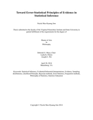
  • 6. List of Figures Figure 1: Axioms for statistical evidence with their logical interrelations................................... 25 vi
  • 7. 1 Introduction Two cognate questions I am tackling in this essay are: (1) what is a genuine principle of evidence? and (2) do error probabilities2 have more than a long-run role? These two questions are related in that my proposed answer to (1) motivates answering “yes” to (2), for reasons that I state in sections 2 and 4. Specifically, defining genuine principles of evidence means determining concepts suitable for interpreting the fundamental properties of statistical evidence (Allan Birnbaum, 1962, p. 270). Such a task requires considering interpretations of, and the rationale behind using, formal or mathematical apparatus (e.g., probability, likelihood). That is, it is important to differentiate the relevant formalism used depending on which statistical framework is employed. To be sure, if one abides by the Bayesian approach then error probabilities are not seen as having more than a long-run role; whereas standing by the frequentist3,4 methodology involves regarding error probabilities as much more than securing low long-run errors. Strictly speaking, error probabilities have been given two additional roles: Allan Birnbaum’s idea of controlling misleading interpretations, and Deborah Mayo’s idea of evaluating a test’s capacity to detect certain errors of interest. Moreover, Birnbaum’s confidence concept (definition 2.1) and Mayo’s severity assessment (definitions 3.1 and 3.2) are closely related, for reasons I develop in section 4. Indeed, Mayo supports Birnbaum’s idea, and I am a proponent of Mayo’s idea. Therefore, the primary goals of this essay are to clarify both Birnbaum and Mayo’s ideas, and to (try to) defend Mayo’s severity evaluation as the most suitable characterization of evidence based on my definition of genuine principles of evidence. 2 An error probability quantifies how probable it is that the method avoids various errors. 3 or the Error-Statistical viewpoint as described in (Mayo & Cox, 2010; Mayo & Spanos, 2011; Mayo, 1996). 4 synonymous with sampling theory. 1
  • 8. 2 Relating principles of evidence to current problems in philosophy of statistics Philosophical debates arise because there is more than one way to construe a concept of evidence. Specifically, assessing how effective a principle of evidence is depends on what statisticians take to be the goal of the inquiry – is it to quantify prior beliefs or prior information? to minimize long-run errors? or to accurately learn aspects of the procedure that generated the data? That is, a principle of evidence is effectual in terms of how well it assists us in fulfilling the aim of the inquiry at hand, whatever the aim might be5 . Furthermore, clarifying (1) what we want to achieve when making inferences, and (2) what a principle of evidence (and the concept of evidence) is, forces statisticians to look more carefully at how particular approaches (e.g., frequentist, Bayesian) regard the nature of statistical inference. If statistical inference is thought to be used as a means for acquiring factual information that simultaneously prevents us from being led astray due to limited information and variability, then probability should be used to quantify how reliable (or capable) a test is of detecting errors. Per contra, if statistical inference is seen as a tool for making decisions (in the decision-theoretic sense6 ), or for guiding people in what to believe, then probability should be used to measure degrees of belief. The most prominent problem in using Bayesian methods is the unwavering emphasis on formalism, which results in paying less attention to the meaning of such abstract entities used in the formalism, along with the rationale for why certain mathematical entities (e.g., prior probability) are the correct apparatus for any one experiment. Due to the growing popularity of the 5 This is why it is crucial to comprehend the differences (and similarities) between various statistical methodologies. However, most proponents of frequentist methods do not have adequate understanding of the Bayesian approach, and vice versa. 6 c.f. (A. Birnbaum, 1977; Lindley, 1977; Wald, 1950). 2
  • 9. Bayesian methodology, the frequentist methodology has been increasingly perceived as failing to provide an account of evidence. In response to this perception of the frequentist approach, my proposed definition of a (genuine) principle of evidence, described in section 3.2, argues for seeing frequentist methods in a new light – vastly different from how they have been traditionally described. 2.1 Birnbaum’s changing views on principles of evidence As the first step to looking at frequentist methods diversely, Birnbaum’s perspective on what counts as a principle of evidence can be seen as an attempt to strengthen the basis for the frequentist approach. The reason for discussing Birnbaum’s view about principles of evidence is Birnbaum was among the first researchers to introduce the notion of a principle of evidence. He is also perhaps the first to raise the question as to whether sampling theory admits of a principle of evidence. In raising this question, Birnbaum proposed something he called the “confidence concept” (1969), which Don Fraser (2004) and Ronald Giere (1977; 1979) have further developed. Definition 2.1 (Birnbaum’s confidence concept (Conf7 )) A concept of statistical evidence is not plausible unless it finds ‘strong evidence for H2 as against H1’ with small probability (𝛼𝛼) when H1 is true, and with much larger probability (1 – 𝛽𝛽) when H2 is true. (A. Birnbaum, 1977, p. 24) To begin with, his earlier work, especially in (1962), leaned toward something akin to “evidential-relationship” (E-R) measures that seek a (logical) relation between statements of evidence and hypotheses. In E-R approaches, as described in (Mayo, 1996), probabilities (or degrees of support or credibility) are assigned to hypotheses. Such degrees of support or credibility purportedly measure strength of evidence for a specific hypothesis. 7 Birnbaum’s confidence concept is a good attempt at ruling out erroneous interpretations of data, but is deficient to denote an adequate concept of evidence, for reasons given in section 3.4. 3
  • 10. Definition 2.2 A statistical hypothesis8 is either (1) a statement about the value of a population parameter (e.g., mean, median, mode, variance), or (2) a statement about the type of probability distribution that a random variable obeys. Still, reading Birnbaum’s most notable expositions on principles of evidence (1962, 1964; 1969, 1972) suggests that he mostly uses “principle” and “axiom” interchangeably, implying that a principle of evidence is mathematical in nature. With the emphasis on mathematics, the mathematical elegance of Bayesian and likelihood-based approaches – defined in section 2.2.3 – attracted him; namely, he found it appealing that these approaches allow “intuitively plausible direct interpretations of all possible numerical values of the likelihood ratio statistic as indicating strength of statistical evidence” (1977, p. 35). Consequently, the Strong Likelihood Principle (LP) quickly became a mathematically compelling way to characterize evidence. Definition 2.3 (Strong Likelihood Principle (LP)) For any two experiments E1 and E2 with different probability models f1Y1 (𝐲𝐲1) and f2Y2 (𝐲𝐲2), but with the same unknown parameter θ, if 𝐲𝐲1 ∗ and 𝐲𝐲2 ∗ are outcomes from E1 and E2 respectively, where the likelihood function of θ given 𝐲𝐲1 ∗ and the likelihood function of θ given 𝐲𝐲2 ∗ are multiples of each other, then 𝐲𝐲1 ∗ and 𝐲𝐲2 ∗ should have identical evidential import for any inference about θ (Mayo, 2013). Definition 2.4 Let 𝐲𝐲 be observations from an experiment, and 𝜃𝜃 be a parameter or hypothesis of interest. Then, 𝑓𝑓(𝐲𝐲|𝜃𝜃) (or ℙ(𝜃𝜃|𝐲𝐲)8F 9 ) is a probability density function when viewed as a function of 𝐲𝐲 with 𝜃𝜃 fixed, and is a likelihood function when viewed as a function of 𝜃𝜃 with 𝐲𝐲 fixed. 8 An example of a statistical hypothesis is: the average body temperature of 15 year olds is greater than 98.6 degrees Fahrenheit. 9 I find this portrayal of a likelihood function to be very misleading because the range of both probability density functions and likelihoods can be outside the interval [0, 1], whereas the range of any probability ℙ(⋅) is – and must lie inside – the interval [0, 1]. At least that is how I understand probability. 4
  • 11. Example of calculating a likelihood function (taken from (Casella & Berger, 2002, sec. 6.3)): Let 𝑋𝑋 ∼ NegBin(𝑟𝑟 = 3, 𝑝𝑝), where 0 ≤ 𝑝𝑝 ≤ 1. If 𝑥𝑥 = 2 then the corresponding likelihood function is: 𝑓𝑓(2|𝑝𝑝) = �4 2 �𝑝𝑝3 (1 − 𝑝𝑝)2 . More generally, if 𝑋𝑋 = 𝑥𝑥 ∈ ℝ, then the likelihood function is: 𝑓𝑓(𝑥𝑥|𝑝𝑝) = �3+𝑥𝑥−1 𝑥𝑥 �𝑝𝑝3 (1 − 𝑝𝑝)𝑥𝑥 . Furthermore, the LP specifies how to use the likelihood function as a “data reduction” device (i.e., converting all information in a data set into fewer dimensions (McGraw-Hill Education, 2002)). In order to understand the LP in the context it was originally intended to be used, another critical assumption underlying the LP is it assumes the statistical model to be adequate, or at least not under question. Definition 2.5 A statistical model10 is an internally consistent set of probabilistic assumptions purporting to provide an adequate (probabilistic) ‘idealized’ description of the stochastic mechanism that gave rise to the observed data with a view to learning about the observable phenomenon of interest (Spanos & McGuirk, 2001, sec. 3.2). That is, a statistical model is defined in terms of its probabilistic assumptions. Example of a statistical model: the simple Normal model [i] 𝑋𝑋𝑘𝑘 ∽ N(𝜇𝜇, 𝜎𝜎2) ∈ Θ ≔ ℝ × ℝ+ , 𝑘𝑘 ∈ ℕ, [ii] (𝑋𝑋1, 𝑋𝑋2, … , 𝑋𝑋𝑛𝑛) are independent [iii] (𝑋𝑋1, 𝑋𝑋2, … , 𝑋𝑋𝑛𝑛) are Identically Distributed However, it is worth noting that Birnbaum later rejected the LP – most notably in (1970) and (1977), as well as “various proposed formalizations of prior information and opinion” (1970), because he later realized that it does not provide theoretical control over error probabilities. 10 It is also worth noting that significance tests can be used for verifying the model assumptions. But I am not able to discuss this topic, due to space and time restraints. For more information on how this is performed, I direct the reader to (Mayo & Spanos, 2004). 5
  • 12. Instead, he ended up being in favor of his proposed “confidence concept” as a principle of evidence that more accurately captures what statisticians do in practice. This change in Birnbaum’s views on principles of evidence is crucial because numerous statisticians still perceive him as being a proponent of the LP. Thus, it is hoped that this change will encourage more statisticians to keep an open mind about various characterizations of statistical evidence, including my proposed definition of genuine principles of evidence. Such open-mindedness is essential to successfully arranging matters in disputes (between Bayesian and frequentist methods), a handful of which is described in the next subsection. 2.2 The Bayesian versus frequentist debate The starting point for defining principles of evidence is in grasping the major differences between Bayesian and frequentist11 methods. Among the several differences between the two methodologies, the one I focus on in this essay concerns the use of probability in statistical inference: the former uses probability to measure “the degree of confidence in a proposition, a quantity varying with the nature and extent of the evidence,” and the later “notes how in ordinary life a knowledge of the relative frequency of occurrence of a particular class of events in a series of repetitions has … an influence on conduct” (Pearson, 1950). As a result, the principles integrated into Bayesian methods lead to appraisals of the “evidential import of data”12 that conflict with error statistical methods. Plainly put, “it is this conflict that is the pivot point around which the main disputes in the philosophy of statistics resolve” (Mayo & Kruse, 2001). Acknowledging and fathoming the discordant perspectives on the role of probability in statistical inference is very pertinent to discussion about principles of evidence, because it manifests contrary ways of interpreting data, in terms of adherence (or lack thereof) to the LP (definition 2.3). 11 or error-statistical; Mayo hopes to replace the phrase ‘frequentist methods’ with ‘error-statistical methods.’ 12 i.e., what the data say or tell us about a hypothesis. 6
  • 13. Complying with the LP implies that the evidential import of the data is through the likelihood. The main reason why the evidential import of the data is through the likelihood – for proponents of the LP – is inference via Bayes’ Theorem entails LP. 2.2.1 Inference via Bayes’ Theorem → LP Theorem 2.6 (Bayes’ Theorem or “Bayes’ Rule” (Casella & Berger, 2002, p. 23).) Let A1, A2, … be a partition of the sample space, and let B be any set that has non-zero Lebesgue measure. Then, for each i = 1, 2, … ℙ(A𝑖𝑖|B) = ℙ�B�A𝑖𝑖�ℙ(A𝑖𝑖) Σ𝑗𝑗=1 ∞ ℙ�B�A𝑗𝑗�ℙ(A𝑗𝑗) . where the sample space consists of all possible outcomes of an experiment. In demonstrating13 the relation between Bayes’ Theorem and LP, let x1 be an outcome from one experiment (experiment 1), and x2 be an outcome from another experiment (experiment 2), with both experiments concerning the same set of hypotheses {𝐻𝐻𝑖𝑖}𝑖𝑖=1 𝑛𝑛 . Then, for each i, the posterior probabilities for the two experiments are: ℙ(𝐻𝐻𝑖𝑖|𝐱𝐱1) = ℙ(𝐱𝐱1|𝐻𝐻𝑖𝑖)ℙ(𝐻𝐻𝑖𝑖) ℙ(𝐱𝐱1) and ℙ(𝐻𝐻𝑖𝑖|𝐱𝐱2) = ℙ(𝐱𝐱2|𝐻𝐻𝑖𝑖)ℙ(𝐻𝐻𝑖𝑖) ℙ(𝐱𝐱2) where ℙ(𝐱𝐱1|𝐻𝐻𝑖𝑖) is the likelihood function for experiment 1, ℙ(𝐱𝐱2|𝐻𝐻𝑖𝑖) is the likelihood function for experiment 2, and ℙ(𝐻𝐻𝑖𝑖) is the prior probability14 of a hypothesis Hi. Subsequently, the ratio of the two posterior probabilities can be expressed as follows: 13 based on (Mayo, 1996, pp. 339–340). 14 often posed as an individual’s assessment – before the data is collected – of how likely a hypothesis is true. 7
  • 14. ℙ(𝐻𝐻𝑖𝑖|𝐱𝐱1) ℙ(𝐻𝐻𝑖𝑖|𝐱𝐱2) = ℙ(𝐱𝐱1|𝐻𝐻𝑖𝑖) ℙ(𝐱𝐱2|𝐻𝐻𝑖𝑖) × c2 c1 = ℙ(𝐱𝐱1|𝐻𝐻𝑖𝑖) kℙ(𝐱𝐱1|𝐻𝐻𝑖𝑖) × c2 c1 = c2 kc1 ∈ ℝ+ 2.2.2 Implications of the LP Notice that the second line of the above equation denotes the following result: that the posterior probabilities are multiples of each other – which is supposed to signify that the two inferences (𝐻𝐻𝑖𝑖|𝐱𝐱1 and 𝐻𝐻𝑖𝑖|𝐱𝐱2) convey the exact same information about each hypothesis Hi (i.e., that 𝐱𝐱1 and 𝐱𝐱2 are “evidentially equivalent” or have “identical evidential import” for any inference about Hi) – under the condition that the likelihood function of Hi given 𝐱𝐱1 is a multiple (e.g., a positive real number k) of the likelihood function of Hi given 𝐱𝐱2. Resultantly, this reading of the equation above is a restatement of the LP. Therefore, LP is a direct consequence of using Bayes’ Theorem. Having shown that the LP follows from inference via Bayes’ Theorem, it is important to note the limitations of this result. The main issue is in holders of the LP appealing to “point against point”15 tests as their leading attempt to defend their argument that the LP can avoid having a high probability of being misled by the data. But in which practical research situations – if any – does the parameter space ever consist of only two points? Definition 2.7 Intuitively, the parameter space is the set of all possible combinations of values for all the (unknown) parameters contained in a particular statistical model (definition 2.5). 15 i.e., the requirement that each hypothesis Hi in the setup in section 2.2.1 must be a simple statistical hypothesis �e. g. , 𝐻𝐻1: 𝑝𝑝 = 1 4 �, because that is the only case where both non-Bayesians and Bayesians agree on calculating the likelihood function (i.e., ℙ(𝐱𝐱1|𝐻𝐻𝑖𝑖) or ℙ(𝐱𝐱2|𝐻𝐻𝑖𝑖)) in the same way when talking about the LP. 8
  • 15. Appealing to point against point tests to defend the LP does not necessarily imply that the LP applies to the more realistic16 case of two-sided tests with vague alternatives (e.g., 𝜇𝜇 ≠ 0); and not being able to apply the argument to actual practice is to their disadvantage. In fact, Birnbaum only retained the LP for point versus point tests, and George Barnard rejected the LP in the most general cases because it gave high error probabilities in the case of a vague alternative. Besides, the LP is essentially nothing more than a mathematical theorem that presumes a specific definition the concepts of “evidential equivalence” and “evidential import of data” (i.e., a concept of evidence) but does not tell us how to interpret statistical evidence or what counts as statistical evidence. For this exact reason, the LP cannot realistically provide appropriate guidance on how to avoid having a high probability of being misled by the data. Accordingly, alluding to the “point against point” test does not actually count toward defending the LP as offering protection in all cases against being misled by the data in more complex cases, as the “point against point” test is not meant to apply to the standard (i.e., more complex) situations encountered in statistical practice. The more complex situations I have in mind are two-sided tests with vague alternatives. To illustrate one instance I have in mind where frequentist methods conflict with the LP, consider Armitage’s example from (Mayo, 1996, pp. 353–354): Let 𝜇𝜇 denote the mean difference in the effectiveness of two drug treatments. Then, the null hypothesis is 𝐻𝐻0: 𝜇𝜇 = 0. The experiment records 𝑋𝑋�, i.e., the mean difference in scores accorded to the two drug treatments in a sample of n patients. The sample size, however, is not fixed but is determined by a stopping rule. Definition 2.8 A stopping rule is the rule or plan from which a researcher decides how much (and what kind of) data to collect for their experiment. 16 or closer to what is encountered in scientific practice. 9
  • 16. In this case, the stopping rule is to keep taking more samples until 𝐻𝐻0 is rejected at the 0.05 significance level (or until |𝑋𝑋�| ≥ 2𝜎𝜎, where 𝜎𝜎 is the (known) standard deviation). (This stopping rule is called optional stopping.) Following this stopping rule, one is assured of obtaining a statistically significant difference at the 0.05 level, even if 𝐻𝐻0 is true. On top of that, ascribing a so-called uninformative or a diffuse prior probability to 𝜇𝜇 would render a low posterior probability to 𝐻𝐻0. Hence, following optional stopping, the Bayesian would be assured of assigning a low probability to 𝐻𝐻0, even though 𝐻𝐻0 is true. Another way of stating the implication of Armitage’s example – specifically for users of Bayesian methods – is the following: because the stopping rule does not alter likelihoods, if the sample size is large enough then proponents of the Bayesian approach are assured (with probability 1) of assigning a low posterior probability (e.g., 0.05) to H0, even though H0 is true. The key insight from this example is the fact that ignoring stopping rules can lead to a high probability of error. In fact, there is even a name for the irrelevance of optional stopping: the stopping rule principle (SRP) (J. O. Berger & Wolpert, 1988, sec. 4.2.1). It is also important to note that “this high error probability is not reflected in the interpretation of data according to the LP” (Mayo & Kruse, 2001, p. 393). Hence, adherence to the LP would not pick up on the fact that one can be wrong with probability 1 in optional stopping with a two-sided test. The most important implication of the LP for the purposes of this essay is its implications for the irrelevance of characteristics indicated by how the data were generated (e.g., stopping rules). As I see it, this implication is what makes it inappropriate to regard the LP as a genuine principle of evidence. What is the use of finding a mathematical characterization of evidence when it cannot help us to profitably describe and interpret the essential properties of statistical evidence? Be that as it may, there is a tendency among proponents of the LP to ignore how the data was 10
  • 17. generated and rely exclusively on how well data agrees with a hypothesis. Such ignorance of the mechanism that generated the data results in looking at error probabilities as having no more than a long-run role, i.e., answering “no” to question (2) stated in section 1. Hence, another prominent difference between the mainstream Bayesian methodology and the error-statistical account is that Bayesians focus only on the observed result after the data is collected because their position is that the evidential import of the data is through the likelihood, while proponents of error-statistical (and frequentist) methods do not restrict themselves to the observed result, in order to get a more complete sense of the capacity17 of a test or estimator in how well it exposes specific errors. Underlying all the instances of relying only on the observed result is “a reluctance18 to allow an experimenter’s intentions to affect conclusions drawn from data” (J. O. Berger & Wolpert, 1988, p. 74). Letting experimenters’ intentions influence interpretation of data seemingly makes a method less objective, where objective typically is understood as not being influenced by personal feelings or opinions in considering and representing pieces of information. Still, such a perspective is anathema to the expectations of a genuine principle of evidence I specify in section 3.2. That being the case, the Bayesians’ emphasis on the observed result lends itself to the previously mentioned implication of the Strong Likelihood Principle (LP): that the sampling distribution is irrelevant to inference once the data is garnered. Definition 2.9 Let Y be a random variable, 𝜃𝜃 be an unknown parameter of interest, and let 𝜃𝜃�(𝒀𝒀) be a test statistic (definition 3.3). Then, the probability distribution of 𝜃𝜃�(𝒀𝒀), when derived 17 A common goal in science is to assess how reliably a test discriminates whether (or not) the actual process giving rise to the data corresponds to that described in hypothesis H, in which case error probabilities may be used to evaluate a “risk” (i.e., possibility of inaccuracy) associated with the predictions H is required to satisfy. 18 This reluctance was a major source of motivation behind establishing the reference (or objective) Bayesian approach described in (J. Berger, 2006; J. M. Bernardo, 2005; José M. Bernardo, 1997). 11
  • 18. from a ‘random sample’19 of size n, is called the sampling distribution20 of 𝜃𝜃�(𝒀𝒀). Put in another way, the sampling distribution is the distribution of 𝜃𝜃�(𝒀𝒀) for all possible samples from the same population of a given size n.. That is, this distinguished implication downplays the data gathering aspect of experiments. Moreover, a noteworthy issue in defining principles of evidence concerns whether knowledge of the stopping rule(s) and sampling distributions are to be taken into account when assessing the evidence from a statistical test. 2.2.3 Synopsis of likelihood and Bayesian methods Having stated the preference – among statisticians21 – for the mathematical elegance of both likelihood-based approaches and the Bayesian methodology, I render a succinct summary of both approaches. The likelihood approach relies solely on likelihood functions for inference and likelihood ratios for comparisons between hypotheses, models, or theories. Such an approach has few advocates, with the most noted ones being (Royall, 1997) and (Sober, 2008). Next, the received view of Bayesian methods is as follows: an unknown (vector of) parameter(s) θ is treated as a random variable itself, which means that a probability distribution is attached to θ. The focus of interest is typically in an unknown constant denoted ψ, usually a component of θ. Defenders of Bayesian methods, in the mainstream use, profess that a degree of belief is used to measure “strength of evidence” or “degree of credibility” that some hypothesis about ψ is true: the bigger the degree of belief, the stronger the evidence is in favor of a hypothesis. 19 a common shorthand for independent and identically distributed. 20 This definition is specific to the context of hypothesis testing, but can be appropriately modified to other contexts as needed. 21 including, but not limited to, Birnbaum. 12
  • 19. The difference between various Bayesian approaches is in their interpretations of prior probabilities. Probability is used in conventional Bayesian methods as an attempt to represent impersonal or rational degrees of belief. In other words, “objectivity in the [conventional] Bayesian approach “is bought by attempting to identify ideally rational degrees of belief controlled by inner coherency” (Cox & Mayo, 2010, p. 277). The motivation behind establishing the conventional Bayesian approach is primarily in responding to the difficulty of eliciting subjective priors, and to the reluctance among researchers to allow subjective beliefs to be conflated with the information provided by the data. Hence, the goal of conventional Bayesian methods is to retain the benefits of the Bayesian approach (e.g., inner coherency, incorporating different types of evidence) while avoiding the problems posed by introducing subjective opinions into scientific inference. Also, a nonmathematical reason for favoring conventional Bayesian methods is the view “that science should embrace subjective statistics falls on deaf ears” (J. Berger, 2006, sec. 2.1): the appearance of the label “objective” [or “conventional”] seemingly makes a method more convincing to users of statistical methods, because statistics is thought to provide objective validation of sciences in general. In contrast, probability is used in subjective Bayesian methods as an attempt to represent personal degrees of belief. Its main appeal in statistical inference comes from a mixture of internal formal coherency with the supposed ability to incorporate evidence of a broader type than that based on frequencies. This ends the overview of Bayesian methods. 2.2.4 Challenges to frequentist methods that Bayesians raise There are more varieties of Bayesianism than before, with no signs of common ground between the extremes. What is more, leading advocates of Bayesian methods – specifically Jim Berger22 and Michael Goldstein23 – disagree with each other about the role of subjectivity in 22 a follower of conventional Bayesian methods. 23 a supporter of the subjective Bayesian approach. 13
  • 20. scientific practice, thus leaving the Bayesian methodology on dubious foundations. For this reason, it is nearly impossible to give a consistent answer to the question of what makes a method Bayesian. Regardless of which type of Bayesianism is applied, one widespread criticism of frequentist methods is that a fair portion of Bayesians takes the aim of significance testing (or hypothesis testing) to be in establishing the probability of a hypothesis. With this supposition in mind, another one of the leading criticisms24 of frequentist methods is that p-values are an ineffective tool for representing effect sizes; and such thinking has led numerous statisticians to doubt the merit of using the frequentist (or error-statistical) approach. Definition 2.10 An effect size is a way of quantifying the size of the difference between two groups, e.g., “the effectiveness of a particular intervention, relative to some comparison” (Coe, 2002). To clarify, effect sizes are used primarily for the purpose of conveying the magnitude (or strength) of some phenomenon, especially when interventions of various types occur, where that phenomenon is explicitly linked to a particular research question (Kelley & Preacher, 2012). It is also worth noting that the notion of effect size is often linked to the idea of substantive significance (e.g., practical, clinical, or medical importance): it is typically understood to be a degree to which interested parties (e.g., practitioners, the public at large) would consider a finding worthy of attention and possibly action. Apparently, the most widely-used representation of effect size among Bayesians is the posterior probability, which leads me to another major criticism of frequentist methods. The Bayesians’ chief criticism of p-values presupposes that a posterior probability is a valid measure of warrant in a hypothesis H. As well, it is crucial to note that proponents of the Bayesian 24 among defenders of Bayesian methods. 14
  • 21. methodology – in the broadest sense – have been unable to agree thus far as to what kind of prior, and thus posterior, is the most suitable measure of warrant in H. 15
  • 22. 3 Attempts at providing genuine principles of evidence 3.1 What a concept of evidence is about A concept of evidence is about controlling and assessing error probabilities, for the purpose of appraising the probabilities of misleading inferences. For this reason, utilizing error probabilities is central to establishing an adequate concept of evidence. Furthermore, providing an adequate concept of evidence would help to avoid misleading inferences, in a way that distinguishes which inferences are defensible from ones that are not. That is, grasping an adequate concept of evidence would encourage more careful scrutiny of which conclusions are (not) warranted by paying more attention to the capabilities of tests to uncover actual errors of interest. Such critical examination is very pertinent to current foundational problems in statistics because, regardless of the discipline and the type of data collected – whether in the humanities or (natural and social) sciences, there is still a pressing need to determine which conclusions or conjectures are valid, and why they are valid. Without an adequate concept of evidence, it is easy to get caught up in the mathematics or more technical components of an experiment, which often leads to losing sight of the goal of performing an inquiry in the first place. 3.2 When is a principle of evidence genuine? The enterprise of supplying genuine principles of evidence is becoming urgently pressing in today’s debates connecting statistical inference, data analysis, machine learning, and general epistemology because even those largely concerned with applications of statistical methods remain interested in identifying general principles that underlie and give grounds for the procedures they respect on practical grounds. Furthermore, it is widely accepted that the common role of statistical methods used across various academic disciplines is to give a framework for learning accurate information about the world with limited data. However, if such a framework is to be settled and 16
  • 23. sustained in practice, then I think that principles and techniques considered to be most useful or apt must contribute to increasing our understanding of the actual processes behind the success25,26 of science. As an attempt to identify general principles that underlie and give grounds for the procedures, I think that felicitous genuine principles of evidence should provide concrete guidelines on precisely how to examine error probabilities, with respect to a test’s aptitude for unmasking pertinent errors, which leads to establishing sound interpretations of results from statistical techniques. For example, Mayo’s severity evaluation yields principles that meet these criteria. The severity assessment is defined as follows: Definition 3.1 A hypothesis H passes a severe test T with data x0 if (S-1) x0 agrees with H (for a suitable notion of “agreement” or “goodness of fit”, where measures of goodness of fit typically summarize the discrepancy between observed values and the values expected under the model in question) and (S-2) with very high probability, test T would have produced a result that accords less well with H than does x0, if H were false or incorrect. Definition 3.2 (Severity Principle (Full)) Data x0 provide a good indication of or evidence for hypothesis H (just) to the extent that the test T has severely passed H with x0. Essentially, the reasoning behind severity is the following: if an agreement between data and hypothesis would very probably have occurred even if the hypothesis is false, then that agreement is poor evidence for that hypothesis. Such guidelines are material for fulfilling the goal 25 From a philosophical perspective, success is in reaching (approximately) true conclusions about aspects of real26 , mostly physical systems; whereas success among practitioners is in acquiring estimators with good properties and small standard errors (i.e., “in solving a data analytic problem” (Kass, 2011, p. 7)). 26 Realism, as I understand it, is defined as the following: “our best scientific theories give true or approximately true descriptions of observable and unobservable aspects of a mind-independent world” (Chakravartty, 2013). 17
  • 24. of making an accurate inference about what exactly is the case regarding a particular phenomenon (i.e., gaining accurate knowledge about (aspects of) a phenomenon), and yet are clearly lacking in the currently used frameworks of statistical practice. Nevertheless, I think that the most constructive way to evaluate a principle is in assessing it on 1) whether and how it applies error probabilities to evaluate the ability of tests to probe prominent errors, and 2) how well it avoids misleading conclusions. According to this definition of genuine principles of evidence, error probabilities have potential to be used to control misleading interpretations (Birnbaum’s idea), and to assess a test’s capacity to uncover certain errors of interest (Mayo’s idea). Moreover, if the primary aim of an experiment is to distinguish between authentic and deceptive results (e.g., whether a correlation is spurious or genuine), then a genuine principle of evidence should explicate exactly which inferences are warranted that are pertinent to the particular research question being asked, and why only those inferences are vindicated. For this reason, the output of a genuine principle of evidence – in the way I defined it – consists of a report of the error probabilities, which hypotheses are valid based on the data, and a rigorous account of why only those hypotheses are justified. 3.3 More on Birnbaum’s confidence concept 3.3.1 Introduction to hypothesis tests As I equip the reader with the necessary apparatus for largely grasping Birnbaum’s confidence concept, as well as why Birnbaum perceives it as a concept of evidence, I present an introduction to hypothesis tests – in the sense of the joint work of Jerzy Neyman and Egon Pearson (1933). The first step in a hypothesis test is to specify a null hypothesis H0 and an alternative hypothesis H1, so that these two hypotheses exhaust the parameter space (definition 2.7). Next, establish a test statistic d(X), as defined below. 18
  • 25. Definition 3.3 Let X be a random variable. Then, a test statistic d(X) is a mapping from the sample space χ = ℝ𝑿𝑿 𝑛𝑛 to the real line: d(X): χ → ℝ, such that χ is partitioned into two mutually exclusive parts: C0 (acceptance region), corresponding to Θ0; and C1 (rejection region), corresponding to Θ1, where (Θ0, Θ1) constitutes an exhaustive partition of the sample space Θ with no overlap between the two regions. After choosing the test statistic, the next step is to determine a pre-data significance level 𝛼𝛼, corresponding to the decision rules laid out below. Definition 3.4 Following the set-up in definition 3.3, Neyman-Pearson decision rules, based on a test statistic d(X), take on the following form after observing data x0: [i] if x0 ∈ C0 then accept H0, [ii] if x0 ∈ C1 then reject H0, and the associated error probabilities are: type I: ℙ(x0 ∈ C1; 𝐻𝐻0(𝜇𝜇0) true) ≤ 𝛼𝛼(𝜃𝜃), for all 𝜇𝜇0 ∈ Θ0, type II: ℙ(x0 ∈ C0; 𝐻𝐻0(𝜇𝜇0) false) = 𝛽𝛽(𝜃𝜃), for all 𝜇𝜇0 ∈ Θ0. Another fundamental concept, power, arises based on the definition of a type II error, because they are inversely related in the following manner: (power) + (type II error) = 1. Hence, larger (smaller) power indicates a lower (bigger) type II error. Definition 3.5 Intuitively, the power of a test is the probability of (correctly) rejecting the null hypothesis when the null hypothesis is false. Using mathematical notation, the power is: 𝜋𝜋(𝜇𝜇1) = 1 − 𝛽𝛽(𝜃𝜃) = ℙ(𝑑𝑑(𝐗𝐗) > 𝑐𝑐𝛼𝛼; 𝐻𝐻0(𝜇𝜇0) false), where 𝜇𝜇1 = 𝜇𝜇0 + 𝛿𝛿, 𝑑𝑑(𝐗𝐗) is a test statistic (definition 3.3), and 𝛿𝛿 > 0 is a discrepancy of interest. Utilizing p-values, we get the following version of the Neyman-Pearson decision rules (cf. definition 3.4): 19
  • 26. Definition 3.6 (N-P decision rule) [i] if 𝑝𝑝(𝐱𝐱0) ≤ 𝛼𝛼 then accept H0; [ii] if 𝑝𝑝(𝐱𝐱0) > 𝛼𝛼 then reject H0. An evidential reading of the N-P decision rule above is: accepting H0 affords insufficient evidence to infer departure from H0, and rejecting H0 bears some evidence of a departure from H0 in the direction specific to alternative H1. The two error probabilities in definition 3.4 are to be interpreted as the probability of rejecting 𝐻𝐻0 when 𝐻𝐻0 is true, and the probability of accepting 𝐻𝐻0 when 𝐻𝐻0 is false, respectively. Thus, a hypothesis test consists of H0 (and its complement), a test statistic, significance level, and the corresponding type II error probability. Birnbaum uses the following symbols to represent statistical evidence: 𝑑𝑑1 ∗ : (reject 𝐻𝐻1 for 𝐻𝐻2, 𝛼𝛼, 𝛽𝛽) and 𝑑𝑑2 ∗ : (reject 𝐻𝐻2 for 𝐻𝐻1, 𝛼𝛼, 𝛽𝛽), which are thought to be “typical interpretations and reports of data treated by standard statistical methods in scientific research contexts” (1977, p. 23). Specifically, 𝑑𝑑1 ∗ is equivalent to “reject 𝐻𝐻1” (or “accept 𝐻𝐻2”) and 𝑑𝑑2 ∗ is equivalent to “reject 𝐻𝐻2” (or “accept 𝐻𝐻1”), with the interpretations being evidential and not behavioral. Distinguishing between behavioral interpretations and evidential interpretations is consequential, which is why I briefly define each of the two types of interpretations in the next subsection. 3.3.2 Behavioral vs. evidential interpretations For dichotomous27 tests, Birnbaum considers the performance of any decision function (e.g., any rule for using data on a sample of lamps from the batch to arrive at a decision d1 or d2) as being characterized fully – under H1 and H2 – by the error probabilities 𝛼𝛼 and 𝛽𝛽, where 𝛼𝛼 = ℙ(𝑑𝑑1|𝐻𝐻1) is the type I error and 𝛽𝛽 = ℙ(𝑑𝑑2|𝐻𝐻2) is the type II error. Here, the first of the two interpretations of decisions is defined: A behavioral interpretation of the decision concept is used 27 I.e., in cases when both the null and alternative hypotheses are simple – in the form H: 𝜃𝜃 = 𝑥𝑥 ∈ ℝ, where 𝜃𝜃 is the unknown parameter of interest. 20
  • 27. to refer to any comparatively simple (i.e., in the context of two point hypotheses), literal interpretation of a decision appearing in a formal model of a decision problem. However, Birnbaum criticizes and rejects this interpretation – he does not find it appropriate in the context of scientific research that utilizes the “standard methods of data analysis” (A. Birnbaum, 1977, p. 22), for the following reason: formulating a problem of testing hypotheses as a problem of deciding28 whether or not to “reject a statistical hypothesis” is unsatisfactory when seeking an evidential interpretation – and not a behavioral interpretation, because the meaning associated with rejecting a hypothesis is unclear. Instead, the decision-like term “reject” calls for providing an evidential interpretation, the second of the two interpretations of decisions: “an interpretation of the statistical evidence [in scientific research contexts], as giving appreciable but limited support to one of the alternative statistical hypotheses” (A. Birnbaum, 1977, p. 23). That is, the meaning of statements of acceptance/rejection (e.g., “reject 𝐻𝐻1”) is called an evidential interpretation, which comprises Birnbaum’s confidence concept. As long as the hypotheses are not all set out in advance, Birnbaum says that the (evidential) interpretations are not decision-theoretic. 3.3.3 Birnbaum’s appraisal of the confidence concept Here is what Birnbaum thinks of the confidence concept – its status in theory and application: There is no precise “mathematical and theoretical system” that guides closely the wide use of the confidence concept in standard practice (A. Birnbaum, 1977, p. 34). He assumed that important concepts for guiding application and interpretation of statistical methods are largely implicit and could not be defined in any systematic theory of inference. In fact, he describes his confidence concept as “a concept whose essential role is recognizable throughout typical research applications and interpretations of standard methods, but a concept which has not been elaborated 28 Although, the behavioral “decisions” made in accordance with Neyman-Pearson hypothesis testing is not tantamount to decision theory with loss functions. 21
  • 28. in any systematic theory of statistical inference” (A. Birnbaum, 1977, p. 28). Notably, the problem of minimization of error probabilities 𝛼𝛼 and 𝛽𝛽 in the context of two simple hypotheses – solved in (Neyman & Pearson, 1933) – leads not to a unique best test or decision function, but to a family of best tests. This is because two simple hypotheses rarely exhaust the parameter space, and therefore multiple combinations of two simple hypotheses are required, in order to cover all possible points in the parameter space. What makes the confidence concept ad hoc – in Birnbaum’s view – is the lack of mathematical/formal elegance, as demonstrated in a generalized kind of test of statistical hypotheses, where a formal decision function takes “three (rather than the usual two) possible values”: d1 – strong evidence for H2 as against H1; d2 – neutral or weak evidence; d3 – strong evidence for H1 as against H2. Thus, “[the decision function] takes the value d1 on those sample points where the test characterized by (0.01, 0.05) would reject H1; it takes the value d3 on those points where the test (0.05, 0.01) would accept H1; and it takes the value d2 on the remaining sample points. Such a “three-decision” test requires a scheme of a new form to represent its more numerous error probabilities (four to be exact in this case – see (A. Birnbaum, 1977, p. 35)). Birnbaum’s appraisal of his proposed confidence concept says much about his attitude about existence of principles of evidence; in particular, it is worth elaborating his thoughts on criteria for evaluating evidence, in light of a highly informative yet unpublished manuscript (1964) and its relation to my definition of a genuine principle of evidence29 . Because no mathematically elegant theory of statistical inference has included the confidence concept in the way Birnbaum defined it, he does not claim that a systematic account containing these important concepts (that would meet my expectations in section 3.2) could be provided – either in this manuscript, or in other articles Birnbaum wrote: “Notwithstanding the evident fact that statistical evidence is very 29 explicated in section 3.2. 22
  • 29. widely and effectively interpreted and used in scientific work, no precise adequate concept of statistical evidence exists – and none can exist, in the sense that precise versions of several very plausible widely-accepted minimum conditions30 for adequacy of such a concept are logically incompatible!” (1964, p. 15). To better understand this noteworthy31 statement in its original context, some definitions are introduced: Definition 3.7 (Unbiasedness criterion for a mode of evidential interpretations (U)) Systematically misleading or inappropriate interpretations shall be impossible; that is, under no 𝜃𝜃 shall there be high probability of outcomes interpreted as ‘strong evidence against 𝜃𝜃’. (Allan Birnbaum, 1964; Ronald N. Giere, 1977, p. 9) “This criterion expresses the Neyman-Pearson interpretation of Fisher’s significance level which was later generalized to include error probabilities of two kinds” (Ronald N. Giere, 1977). Nevertheless Birnbaum goes on to argue that U is incompatible with C (conditionality – definition 3.8) and thus with L (strong likelihood – definition 2.3). Put in another way, “[i]t seemed to Birnbaum that there was a broad consensus among statisticians that any adequate conception of statistical evidence should include both U and C – both control over error probabilities and conditioning as ruling out irrelevant outcomes. But he had shown that this is impossible” (Ronald N. Giere, 1977, p. 9). Definition 3.8 (The conditionality axiom (C)) If an experiment E is (mathematically equivalent to) a mixture G of 𝑚𝑚 ∈ ℝ+ components {𝐸𝐸ℎ}ℎ=1 𝑚𝑚 , with possible outcomes {(𝐸𝐸ℎ, 𝑥𝑥ℎ)}ℎ=1 𝑚𝑚 , then Ev�𝐸𝐸, (𝐸𝐸ℎ, 𝑥𝑥ℎ)� = Ev(𝐸𝐸ℎ, 𝑥𝑥ℎ). (Allan Birnbaum, 1962, p. 279) 30 such as the Strong Likelihood Principle (definition 2.2), and his confidence concept. 31 This is not Birnbaum’s ultimate view (on principles of evidence); however, my reason for considering the quote from (Allan Birnbaum, 1964, p. 15) is because it illuminates the discordant attitudes around the conditions for an adequate concept of evidence. 23
  • 30. However, recent studies (Mayo, 2010, 2014a) have shown that Birnbaum’s proof32 is flawed. (Hence, U and C are not necessarily incompatible, or at least there is no compelling evidence for the claim that U and C conflict each other.) To help the reader get the gist of Birnbaum’s proof, a few more definitions are necessary. Definition 3.9 Let Y be a random variable with observed value y, and 𝜃𝜃 be the parameter of interest. Then, s is a sufficient statistic33 if the following factorization holds: 𝑓𝑓𝑌𝑌(𝐲𝐲; 𝜃𝜃) = 𝑚𝑚1(𝐲𝐲)𝑚𝑚2(𝐬𝐬; 𝜃𝜃) where m1 does not involve 𝜃𝜃 and m2 is a function of s. Definition 3.10 A statistic s is minimal sufficient if 1. s is a sufficient statistic, and 2. if t(y) is sufficient then there exists a function g such that s = g(t(y)). Definition 3.11 (The sufficiency axiom (S)34 ) If s is minimal sufficient for θ in experiment E and 𝐬𝐬(𝐲𝐲1) = 𝐬𝐬(𝐲𝐲2) then the inference from 𝐲𝐲1 and 𝐲𝐲2 about θ should be identical. In other words, the idea behind sufficiency is that all the information about 𝜃𝜃 contained in the data is obtained from considering a statistic S(Y) = s(y) with its sampling distribution 𝑓𝑓S(𝐬𝐬; θ) (definition 2.9). Acknowledging that Birnbaum’s proof is unsound is crucial because it opens the door to (new) foundations that are free from paying homage to the strong likelihood principle (Mayo, 2014b). Nevertheless, the central result of Birnbaum’s earlier considerations, and the best representation of Birnbaum’s attitude on principles of evidence, is a trilemma concerning the concept of statistical evidence: “The only theories which are formally complete, and of adequate scope for treating statistical evidence and its interpretations in scientific research contexts, are 32 that (S and C)→L; i.e., that sufficiency + conditionality → the likelihood principle. 33 Lehmann and Scheffé (1950) have equipped us with a procedure to (readily) derive sufficient statistics for more general families of probability densities – not only for Euclidean spaces or very simple cases. 34 corresponds to Lemma 1 in (Allan Birnbaum, 1962, p. 278). 24
  • 31. Bayesian; but their crucial concept of prior probability remains without adequate interpretation in these contexts. Each of the non-Bayesian alternatives, one identified with the likelihood concept and the other with the error probability concept, seems an essential part of any adequate concept of evidence, but each separately is seriously incomplete and inadequate; however, these cannot be combined because they are incompatible.” (1964, 37-38). My short analysis of the trilemma is as follows: the first part about Bayesian methods explains Birnbaum’s high regard for L in (1962), since L follows from Bayes’ theorem – see Figure 1. Figure 1: Axioms for statistical evidence with their logical interrelations (Allan Birnbaum, 1964). At the same time, he acknowledges that priors are not given precise interpretations, which is still an open problem today. His reluctance to accept L is captured well in the following quote: “For those inclined to accept the likelihood concept for experimental evidence, such an extension of the likelihood concept would seem particularly attractive; but its value depends of course on an answer to questions of interpreting likelihood functions [defined in definition 2.4] in general.” (1964, 37). For the second part on the non-Bayesian alternatives, interpretation of both likelihood 25
  • 32. functions and error probabilities was (and still is) “inadequate” when using the most current statistical frameworks, in the sense that the justification and rationale for using these mathematical quantities in the first place (to achieve specific goals) is unsettled among statisticians – not yet agreed upon. Despite Birnbaum’s later rejection of evidential-relationship (E-R)35 approaches (e.g., the “likelihood concept” in (1970; 1977)), he does not indicate in his work that the confidence concept provides all the tools we need to interpret statistical evidence, which implies that something more is needed. On the other hand, Birnbaum could not anticipate in advance what more was needed, at least during his later writings in the 1970s. Nevertheless, Birnbaum’s confidence concept is a good starting point for my definition of genuine principles of evidence. To elucidate what more needs to be done, I give precise reasons why Birnbaum’s confidence concept itself is inadequate for the purpose of supplying genuine principles of evidence. 3.4 Why Birnbaum’s confidence concept is not enough For one thing, the error probabilities used in Birnbaum’s confidence concept are pre-data, as opposed to post-data. This distinction is imperative because it is typically after data collection that a researcher is interested in making inferences. Also, Birnbaum’s confidence concept, like other conventional mathematical quantities (e.g., power) that are commonly used, is independent36 of the actual outcome. For example, Birnbaum interprets (reject H2 for H1, 0, 0.2) as “weak evidence for H1 as against H2” (1977, p. 25), due to the “relatively large value 0.2 of the error probability of the second kind.” That is, Birnbaum’s interpretation rests solely on the fact that the type II error probability is large (i.e., 0.2) whereas the type I error probability is small (e.g., 0.03 in the example that follows). But using only pre-data error probabilities would not pick up on the 35 introduced in section 2.1. 36 because the power is sensitive to the sample size but is based on a cut-off rather than the actual outcome. 26
  • 33. test’s ability to detect a discrepancy of interest (e.g., 𝛿𝛿 = 0.6) – even if the discrepancy exists – with respect to the actual outcome. To illustrate this, consider a one-sided Normal test 𝑇𝑇0.03 with the following hypotheses: H0: 𝜇𝜇 = 0 vs. H1: 𝜇𝜇 > 0, at significance level α = .03 and sample size n = 25. Then, the cut-off for rejection is 𝑥𝑥̅ > 0.4. Now examine a particular alternative with the following hypotheses H2: 𝜇𝜇 = 0.6 vs. H3: 𝜇𝜇 > 0.6. In this (modified) case, the test statistic 𝑍𝑍 = (𝑥𝑥̅−0.6) 1 √25 = 5(𝑥𝑥̅ − 0.6), where 𝑥𝑥̅ ∼ 𝑁𝑁(0.6, 1) under H2. Let this particular test 𝑇𝑇0.03 with data x0 yield the following result: 𝑥𝑥̅ = 0.4 ⇔ 𝑍𝑍 = 5(0.4 − 0.6) = −1, so we would ‘Accept H2’ because the cut-off for rejection is 𝑥𝑥̅ > 0.4. The severity (definitions 3.1 and 3.2)37 is 𝑆𝑆𝑆𝑆𝑆𝑆(𝑇𝑇0.03, 𝐱𝐱0, 𝜇𝜇 ≤ 0.6) = ℙ(𝑍𝑍 > −1; 0.6) = 1 − 0.1587 = 0.8413. However, let us see what happens when the observed 𝑥𝑥̅ were closer to the null (𝜇𝜇 = 0); in other words, now consider the case 𝑥𝑥̅ = 0. In this particular case, the test statistic 𝑍𝑍 = 5(0 − 0.6) = −3, and the severity is: 𝑆𝑆𝑆𝑆𝑆𝑆(𝑇𝑇0.03, 𝐱𝐱0, 𝜇𝜇 ≤ 0.6) = ℙ(𝑍𝑍 > −3; 0.6) = 1 − 0.0013 = 0.9987. What the above calculations demonstrate is that the test 𝑇𝑇0.03 has high capability to detect the discrepancy 𝛿𝛿 = 0.6, if it is present. Furthermore, the outcomes 𝑥𝑥̅ = 0.4 and 𝑥𝑥̅ = 0 constitute pretty good evidence that 𝜇𝜇 ≤ 0.6, which is in contrast to Birnbaum’s interpretation: “weak evidence for [𝐻𝐻2: 𝜇𝜇 = 0.6] as against [𝐻𝐻3: 𝜇𝜇 > 0.6].” The main lesson to take from this example is that pre-data error probabilities do not pick up on a test’s ability (or lack thereof) to unearth a discrepancy 𝛿𝛿, with respect to the actual outcome. Being able to pick up on a test’s capability is 37 Another example of how to calculate severity is given in section 4.1.2. 27
  • 34. crucial in appraising the severity – to figure out exactly which discrepancies can or cannot be ruled out when failing to reject the null hypothesis. 3.5 What would be needed to improve the situation in statistical foundations As a progressive step to improving the current situation in foundations of statistics, I urge practitioners and teachers of statistics to use the existing38 literature with critical attention to ways in which it is incomplete or weak. Put in another way, statistics as a profession or discipline would benefit greatly from developing a more “varied applied methodological literature; but it must include at least some critical and systematic discussions of specific applications of concepts and techniques, as these do or do not appear appropriate (a) in relation to the subject matter and problems under investigation; (b) in relation to one or more of our systematic theories of statistical inference; and (c) overall” (Allan Birnbaum, 1971, p. 16). Examining statistical concepts with some skepticism is useful for clarifying the scope or limits of certain techniques, and for developing more precise definitions of prevailing concepts, including prior and posterior probabilities. A systematic and critical study of statistical concepts also would yield a clearer distinction between what questions or problems statistics is used for addressing in numerous application areas versus what types of questions statistics as a discipline itself is capable of answering. That is, there is a need to elucidate the role “statistics” plays in various research areas that make use of statistical methods. Doing so would bring greater clarity to statisticians and educators about why we use certain statistical techniques, why and how those techniques work (or not), and how to most accurately interpret results that those techniques yield. Lastly, a good starting point for examining important statistical concepts is to apply Mayo’s severity evaluation in practice. 38 including Mayo’s severity evaluation and my definition of (genuine) principles of evidence, which are not in the “standard” statistics literature. 28
  • 35. 4 How an error-statistical account provides a concept of evidence With the desiderata for interpreting statistical evidence set forth in section 3.2, this section seeks to qualify Deborah Mayo’s severity evaluation (definitions 3.1 and 3.2) as an instrument that properly guides us on exactly how to examine error probabilities, with respect to a test’s aptitude for unmasking pertinent errors, as well as how to preclude misleading inferences. Particularly, the setting I have in mind is in performing research that aims to produce comprehensive theories that yield (approximately) true descriptions of complex physical systems that are in the world we live in. Further, I concentrate on hypothesis testing, as opposed to parameter estimation or other problems of interest in statistical practice. In this setting, a widely accepted goal is to gain accurate and reliable knowledge about aspects of a phenomenon in the face of partial or incomplete information. 4.1 Mayo’s severity evaluation as a characterization of evidence To help us distinguish whether the knowledge we obtain is dependable or deceptive, the rationale behind severity is that error probabilities may be used to make inferences about the data gathering process, in light of the observed data x0, by enabling assessment of how well probed hypotheses are (Mayo & Spanos, 2006, p. 328). Hence, error probabilities have much more than a long-run role, i.e., answering “yes” to question (2) stated in section 1. Notice the emphasis on the process behind data collection. Considering the differences between Bayesian and frequentist methods stated in section 2.2, this emphasis is fundamental when it comes to choosing which statistical method to use for a given task. When choosing which statistical method to use, the primary factors should be 1) whether and how it utilizes error probabilities to evaluate the ability of tests to probe prominent errors, and 2) how well it avoids misleading conclusions – not how well it accords with our acumen. Recall that complying with the Strong Likelihood Principle 29
  • 36. (definition 2.3) does not enable control of error probabilities, provides no means for assessing capability of tests, nor is it shown that it effectually rules out deceptive conclusions or conjectures. Without any delay, here are my main reasons for why the severity assessment yields the most appropriate conceptualization of evidence: it (1) emphasizes interpretation rather than focusing exclusively on formalism/mathematics, (2) blocks out bad inference, and (3) avoids fallacies. Of course, a statistical methodology of any kind involves some formalism (e.g., probability), but placing higher value on interpretation can make plain the role39 of probability in statistical inference. The formalism utilized in the severity assessment primarily consists of error probabilities. With appropriate emphasis on interpretation, a key feature unique to the severity assessment is that the interpretations it renders are sensitive to the actual outcome (i.e., the sample size and the value of the test statistic under the observed data). This is because the comparison of obtaining a result that “accords less well” in second condition (S-2) is with respect to the actual outcome (x0). Another way of articulating the second condition (S-2) in definition 3.1 gives rise to a general frequentist principle of evidence (FEV (i)) for detecting where there is strong evidence for a statistical hypothesis (of the 5 types listed in (Mayo & Cox, 2010, sec. 3.1)): Definition 4.1 (FEV (i)) Data y is (strong) evidence against hypothesis H0 if and only if a less discordant result would be observed than is exemplified by y with high probability, given that H0 correctly describes the mechanism that generated y. Mayo’s severity evaluation is one of the few tools available that comes to the aid of avoiding (at least) two persistent fallacies, namely the fallacy of acceptance and the fallacy of rejection. 39 There is benefit to grasping the various ways probability is used in inference, because the idea of quantifying uncertainty in some form is ubiquitous. 30
  • 37. Definition 4.2 Fallacy of acceptance: lack of evidence against H0 is misinterpreted as evidence for H0. Definition 4.3 Fallacy of rejection (i): evidence against H0 is misinterpreted as evidence for a particular alternative H1, at parameter values beyond what is warranted via the severity evaluation. Definition 4.4 Fallacy of rejection (ii): a statistically significant result is misinterpreted as being substantively significant. Succinctly, the severity evaluation addresses both fallacies by indicating precisely which discrepancies from the null hypothesis are warranted with very high severity and which are not40 . 4.1.1 Why severity is a genuine principle of evidence Besides, the data-dependence aspect is what makes the severity assessment a genuine principle of evidence in the way I defined41 it: the performance of a hypothesis test (e.g., the capability of detecting a spurious correlation) is evaluated in terms of what discrepancies it is capable of revealing in the specific case at hand. That is, when one takes into account both the sample size and the calculated value of the test statistic, grasping a test’s capacity to reveal inconsistencies and discrepancies (in the respects probed) then gives us a systematic way of warranting whether there is strong evidence against H in that particular case. Another crucial aspect of the error-statistical approach is the appreciable use of counterfactual reasoning in evaluating how well-tested a claim is in light of the particular data: type I and type II error probabilities are precisely interpreted as evaluations of the sampling distribution of d(X) under different scenarios relating to various hypothesized values of a parameter 40 Additionally, I give a numerical example in section 4.1.2 to indicate how the severity evaluation avoids the fallacy of acceptance. 41 in section 3.2. 31
  • 38. 𝜃𝜃. Taking into consideration all the various scenarios, along with applying FEV (i) (definition 4.1), is how the severity assessment supplies a way for us to block out bad inference. Additionally, the following example illustrates one instance of how to calculate severity. (This example also serves to demonstrate counterfactual reasoning that aids in distinguishing chance effects from genuine effects.) 4.1.2 Example of calculating severity A numerical example that illustrates avoiding the fallacy of acceptance: Company A proposes the take-over of Company B. Let p denote the actual proportion of Company B’s shareholders who are in favor of the offer. Then, consider the following hypotheses: H0: 𝑝𝑝 = 0.50 (claim of Company B’s Chief Executive), vs. H1: 𝑝𝑝 > 0.50 (claim of Company A’s Chairman; one-tailed). at significance level α = .01, with 𝑝𝑝̂ ∼ 𝑁𝑁 � 200 400 = 0.50, 100 4002 = 0.000625� 42 under H0 and sample size n = 400. Accordingly, the test 𝑇𝑇𝛼𝛼 = {d(X), C1(α)} is of the form: test statistic: d(X) = (𝑝𝑝�−0.50) √0.000625 = 40(𝑝𝑝̂ − 0.50), where 𝑝𝑝̂ = 𝑋𝑋 𝑛𝑛 and 𝑋𝑋 ∼ 𝑁𝑁(200, 100) under H0, rejection region: C1(α) = {x0 : d(x0) > 𝑐𝑐𝛼𝛼 = 2.326 ⇔ 𝑝𝑝̂ ≥ 0.55815}. Let test 𝑇𝑇𝛼𝛼 with data x0 yield the following result: d(x0) = 2, 𝑝𝑝̂ = 221 400 = 0.5525, so we would ‘Accept H0’ because the cut-off for rejection is 𝑝𝑝̂ = 0.55815. Suppose Company B’s Chief Executive makes the following assertion: ‘We may infer that any discrepancy from 0.50 is absent or no greater than 0.025’ ⇔ ‘𝑝𝑝 ≤ 0.5025.’ 42 I choose to use the normal distribution in this case because a normal/Gaussian distribution usually provides a good approximation to a binomial distribution when 𝑛𝑛 ≥ 50 and 0.1 ≤ 𝑝𝑝 ≤ 0.9. 32
  • 39. In order to correctly examine whether Company B’s Chief Executive is misinterpreting a lack of evidence for H0 as providing evidence for H0, the pertinent question to ask is: How severely does test 𝑇𝑇𝛼𝛼 pass the hypothesis ‘𝑝𝑝 ≤ 0.5025’ with 𝑝𝑝̂ = 0.5525? The answer is: SEV(𝑇𝑇α, 𝑑𝑑(𝐱𝐱0) = 2, 𝑝𝑝 ≤ 0.5025) = ℙ(𝑑𝑑(𝐗𝐗) > 2; 𝑝𝑝 > 0.5025) = ℙ(𝑍𝑍 > 2) = 0.0228 where Z is a random variable obeying the Normal/Gaussian distribution with mean 0 and variance 1. The accurate way to interpret the severity calculation above is: this statistically insignificant or larger result would occur 97.72% of the time, even if a discrepancy of 0.025 from H0 exists. Due to the high error probability (i.e., 97.72%), the inference that Company B’s Chief Executive makes, ‘𝑝𝑝 ≤ 0.5025,’ is not warranted, thus indicating that the result d(x0) = 2 is poor evidence for the hypothesis ‘any discrepancy from 0.50 is absent or no greater than 0.025.’ Such reasoning is captured by the Severity Interpretation of Acceptance (SIA): “If a test has a very low probability to detect the existence of a given discrepancy from [hypothesized value] 𝑝𝑝, then such a negative result is poor evidence that so small a discrepancy is absent” (Mayo & Spanos, 2006, p. 339, substituted p for their µ0). Thus, failing to reject H0 in this particular test would not let us rule out the discrepancy 𝛿𝛿 = 0.025, because the test does not have enough capacity to detect the discrepancy 𝛿𝛿 even if the discrepancy is existent! Therefore, avoiding the fallacy of acceptance entails denying the assertion made by Company B’s Chief Executive. In avoiding these three fallacies, the severity evaluation promotes a correct logic of an entire inquiry from experimental design to drawing the conclusion. Thus, it meets my expectations for providing genuine principles of evidence, which render rigorous interpretations of statistical evidence. 33
  • 40. Toward satisfying the goal of supplying genuine principles of evidence, using the severity assessment, together with the N-P decision rule (definition 3.4), brings about the opportunity to vindicate claims pertaining to the “strength” of evidence (i.e., weak or strong) for certain departures from H0 in a way that avoids classic fallacies that come with misunderstanding the meaning of rejecting and accepting H0. 4.2 How severity relates to Birnbaum’s confidence concept At this point, it is worth noting a key similarity between Birnbaum’s confidence concept and Mayo’s severity evaluation: both approaches highlight the value of controlling error probabilities. Hence, there are benefits of the error-statistical approach with respect to Birnbaum’s confidence concept. When compared to the confidence concept, likelihood and Bayesian approaches offer attractive features of systematic precision and generality, but fail to provide a kind of (theoretical) control over the error probabilities akin to what the confidence concept (or Mayo’s severity assessment) affords. What is more, the ability to control error probabilities played a very important role in Birnbaum’s development43 of the confidence concept, in which he concentrated exclusively on evidential interpretations; and yet the goal of controlling long run error probabilities is more suitable for a behavioristic reading of statistical methods, “wherein tests are interpreted as tools for deciding “how to behave” in relation to the phenomena under test, and are justified in terms of their ability to ensure low long-run errors” (Mayo & Spanos, 2011, p. 163). This suitability comes from low long run errors alone being a sound basis for behavioristic interpretations, whereas low long run errors alone are not enough for evidential interpretations. 43 Indeed, he acknowledged the utility of error probabilities: “In typical current practice, some reference to error- probabilities accompanies inference statements (“assertions,” or “conclusions”) about parameter values or hypotheses” (Allan Birnbaum, 1962, p. 276). 34
  • 41. 4.3 Where this leaves us in the current situation about foundations of statistics Notwithstanding the conflicts of interest between Bayesian and frequentist approaches, especially the differences mentioned in section 2.2, both approaches agree that evidence is a concept central to understanding the nature and role of statistical methods. In light of the import of evidence as a concept, very little has been accomplished in terms of determining concepts suitable for interpreting the fundamental properties of statistical evidence. Rather, an irrelevant44 question that continues to receive ample attention – both among philosophers of science and practitioners of statistics – is: which mathematical quantity (e.g., p-value, likelihood ratio), if any, truly adequately represents strength of evidence for a specified hypothesis or research question? 4.3.1 Responses to challenges that Bayesians raise For any mathematical entity (e.g., posterior probability, p-value), the question isn’t getting the formal definition down, but rather the relevance of such a computation for the case at hand. Many researchers might think they want a posterior simply because they do not see how to use error probabilities (i.e., probabilities that quantify a method’s capability to avoid various errors) in appraising evidence in the case at hand. But lacking a suitable definition of the prior and posterior probabilities, this leaves researchers very puzzled about the justification of statistical methods as evidence. Besides, genuine principles of evidence highlight the need to consider the rationale behind using these statistical tools – not just the mathematics underlying those tools. Thus far, the development of Bayesian methods has not paid much attention to establishing the rationale behind and interpretation of statistical tools. As a proponent of the error-statistical perspective, I consider a measure of evidence in a hypothesis H to be based on an appraisal of how well-tested H is, with 44 to developing genuine principles of evidence – guidelines that aid researchers in determining exactly what information counts as evidence for (or against) a hypothesis. 35
  • 42. respect to the data-generating mechanism. Such a measure of evidence in H is most suitably established by considering the associated error probabilities. In response to the untiring resistance to the error-statistical approach, especially the criticisms mentioned in section 2.2.4, I maintain that the severity assessment (introduced in section 3.2) is easily able to provide a representation of effect sizes. As with every hypothesis test45 , there are two cases to distinguish from: statistically significant results and statistically insignificant results. Due to the behavioristic interpretations given to the Neyman-Pearson framework over the years, the former case is associated with rejecting the null hypothesis H0, while the latter case is associated with accepting H0. Attaching an evidential interpretation, however, requires going beyond mere acceptance or rejection of H0 in the following way. When rejecting H0, one minus the power of the test at a point 𝜇𝜇1 = 𝜇𝜇0 + 𝛾𝛾 – where 𝛾𝛾 ≥ 0 is a discrepancy of interest and 𝜇𝜇0 is the hypothesized value of an unknown parameter 𝜇𝜇 – provides a lower bound for the severity for the inference ‘𝜇𝜇 > 𝜇𝜇1’. Or, in the case of rejecting H0, the relation between power (definition 3.7) and severity (definitions 3.1 and 3.2) becomes the following: “The higher the power of the test to detect discrepancy 𝛾𝛾, the lower the severity for inferring 𝜇𝜇 > 𝜇𝜇1 on the basis of a rejection of H0” (Mayo & Spanos, 2006, p. 345). Per contra, in cases of accepting H0, the power of a test against 𝜇𝜇 = 𝜇𝜇1 is an upper bound for the severity of a claim ‘𝜇𝜇 ≤ 𝜇𝜇1’ based on a (just) non-significant result. In these cases, the shape of the power curve is the same as that of the severity curve: mathematically, the two behave the same way. To sum up the depiction of effect sizes thus far, properly using the severity concept to report effect sizes means considering the lower bound if the result is statistically significant, or considering the upper bound if the result is statistically insignificant result. 45 For simplicity, I consider one-sided tests instead of two-sided tests. On the other hand, my exposition of the severity assessment could be accommodated in two-sided tests. 36
  • 43. However, using severity to report effect sizes does not imply discarding the p-value altogether. Rather, the p-value has an important role to play in making inferences. The p-value is a post-data error probability, and is to be accompanied by interpretive tools that avoid fallacies46 by highlighting the correct logic of hypothesis tests. Depending on the type of test conducted, the interpretation of the p-value differs accordingly. For a Fisherian test, the p-value is a measure of inconsistency between what is expected and what is observed in the sense that smaller p-values imply more discordance between data x0 and hypothesis H0 (Cox, 1958). Understanding the reasoning of Fisherian tests requires distinguishing between two cases: if the p-value is not small then the disagreement is not considered strong enough to indicate evidence of departures from H0; while if the p-value is small enough then x0 is taken as grounds to reject or find a discrepancy from H0. Whether the p-value is small enough or not depends on the context of the research question being investigated. When using Fisherian tests, the severity assessment then allows researchers to precisely measure the discordance between x0 and H0 as a way of assessing the amount of evidence for or against a particular H0. For the Neyman-Pearson (N-P) test, p-values are commonly interpreted in accordance with the N-P decision rule (definition 3.6). Regardless of the type of test conducted, Mayo’s error-statistical account supplies a genuine principle47 of evidence that explicitly considers the case48 of statistically insignificant results (i.e., moderate to large p-values), namely FEV(ii) introduced in (Mayo & Cox, 2010, p. 256). Definition 4.5 (FEV (ii)) A moderate p value is evidence of the absence of a discrepancy δ from H0, only if there is a high probability the test would have given a worse fit with H0 46 Unfortunately, space does not permit me to go through all the classic fallacies. Although, (Mayo & Spanos, 2011) is an excellent reference that thoroughly goes over several of those fallacies. 47 Yes, it meets the expectations I outline. At this point, it is worth noting that all of the principles of evidence in the error-statistical methodology exemplify genuine principles of evidence in the way I define them. 48 that all the other statistical frameworks used regularly in practice do not provide, due to the pronounced weight given to statistically significant results. 37
  • 44. (i.e., smaller p value) were a discrepancy δ to exist. Moreover, when p-values are used via FEV(ii), p-values can then be used as a basis for inferring genuine results. 4.3.2 Making headway in developing an adequate concept of evidence There may or may not be a unanimous answer to whether there is a mathematical quantity that truly adequately represents strength of evidence for a specified hypothesis, but I find such an enterprise to be misplaced because a mathematical quantity itself does not matter as much as the interpretation attached to it. The lack of attention paid to establishing accurate interpretations (e.g., of a p-value) is evident in the form of classic fallacies, such as the fallacy of acceptance (definition 4.4) and the fallacy of rejection (definitions 4.5 and 4.6). In contrast to finding a quantitative measure of (strength of) evidence, what I think is needed to opportunely achieve the goal of supplying genuine principles of evidence, and therefore discern evidence as a key concept, is an assortment of precise guidelines that tell us how to make sense of (statistical) evidence – how to examine error probabilities, with respect to a test’s aptitude for unmasking pertinent errors, which leads to establishing sound interpretations of results from statistical techniques. Thus, focusing on interpretations of, and rationale behind using, statistical methods is a dependable way to clearly spell out what it is that we want to achieve when making inferences, as well as how to choose felicitous apparatus for making warranted inferences that prevent us from being misled by the data. 38
  • 45. 5 Conclusion In this essay, I offered a definition of a genuine principle of evidence, elucidated Birnbaum’s confidence concept (definition 2.1) and Mayo’s severity evaluation (definitions 3.1 and 3.2), and attempted to defend Mayo’s severity evaluation as the most suitable characterization of evidence based on my definition of genuine principles of evidence. Birnbaum’s changing attitudes regarding what counts as a principle of evidence can be seen as an attempt to strengthen the basis for the frequentist approach. This is because he eventually realized the value of having control over error probabilities. Furthermore, the error-statistical approach, along with Birnbaum’s confidence concept, yields a radically different way of looking at error probabilities: in addition to having a long-run role, error probabilities have potential to be used to control misleading interpretations (Birnbaum’s idea), and to assess a test’s capacity to uncover certain errors of interest (Mayo’s idea). These two ways of utilizing error probabilities, along with my recommended definition of genuine principles of evidence, constitute a unique take on the frequentist methodology that is radically divergent from the traditional means used to introduce frequentist methods in the current statistics curriculum. 5.1 How philosophical issues arise in statistical education Philosophical issues may not be obvious or come up often (explicitly) when teaching statistics, but I do think that philosophical issues arise at least implicitly in statistical education whenever professors or teachers try either to present frequentist and Bayesian approaches side by side, or to contrast (and compare) the two methodologies against each other. In contrast to what many educators and statisticians think49 , the Bayesian and frequentist approaches are vastly 49 Yes, a fair portion of statisticians believes that much if not most of the time the two perspectives (i.e., Bayesian and frequentist) will agree if constructed under the same assumptions (model) and interpreted properly. 39
  • 46. different in their aims and the way they see statistics being used in (natural or social) science, especially when one looks more carefully at the foundations of each methodology (e.g., disagreements about where exactly probability enters into inference, or about what counts as relevant information). This realization is pivotal to fully grasping the limitations of the widely- used Strong Likelihood Principle (LP – definition 2.3) that has raised much controversy in scientific practice, as well as other mathematical characterizations of evidence. Moreover, considering the merit of the LP with respect to my proposed definition of principles of evidence is my initial step to helping educators and statisticians clear up any misunderstanding of the various attempts to quantify evidence – including the widely-used LP. For many years, statistics has typically been taught as a branch of mathematics, in a way that emphasizes performing computations and memorizing formulae. Instead, an approach that emphasizes “interpretations of evidence”50 would prepare and encourage students to take adequate care in how results are presented (and interpreted), and in how conclusions are drawn. Additionally, it is worth noting that there has been much effort recently to focus attention on developing students’ capability to think statistically. For example, the current guidelines for assessment and instruction in statistics education (GAISE) report acknowledges the “importance of giving more people a sounder grasp of the fundamental concepts needed to use and interpret those tools intelligently51 ” (American Statistical Association, 2010). More specifically, one of the recommendations in the current GAISE report is to underscore conceptual understanding, and pay less attention on technical or mathematical understanding. What is more, concepts are defined in 50 i.e., “determining concepts and terms appropriate to describe and interpret the essential properties of statistical evidence” (Allan Birnbaum, 1962). 51 i.e., with a (somewhat) critical attitude toward statistical methods, in terms of not taking everything for granted, or not being afraid to question the basis for anything one learns. 40
  • 47. the context of a particular methodology52 . That is, the methodology and philosophy together provide the framework in which the concept is explained. With several competing methodologies being used in practice, however, it is vital to grasp similarities and differences between methodologies. Ergo, philosophical topics will inevitably emerge as more and more educators encourage conceptual understanding53 , as well as comparisons between dissonant approaches to statistical inference. 5.2 Other implications my definition of genuine principles of evidence A noteworthy implication of my definition is that the popular Strong Likelihood Principle (LP – definition 2.3) does not count as a genuine principle of evidence. This is because the LP does not yield concrete guidelines for describing and interpreting statistical evidence. Rather, I demonstrated that the error-statistical approach – particularly Mayo’s severity evaluation (definitions 3.1 and 3.2) – provides genuine principles of evidence (e.g., FEV (i) – definition 4.1), in the sense that it provides us concrete guidelines on precisely how to examine error probabilities, with respect to a test’s aptitude for unmasking pertinent errors, as well as how to avoid deceptive conclusions. Such principles of evidence are based on sampling theory54 . For reasons stated mainly in section 4, this way of interpreting evidence is the most appropriate conceptualization of evidence when the goal of an experiment is to acquire accurate and reliable knowledge about aspects of a phenomenon in the face of partial or incomplete information. Also, the error-statistical 52 and the corresponding philosophy. 53 Although I think Mayo’s general philosophy is a promising way to help students and educators improve their conceptual understanding, the error-statistical approach has not been developed to the degree that it can readily be merged with methods used for assessing statistical reasoning, such as the Structure of Observed Learning Outcomes model (Biggs & Collis, 1982) and a Comprehensive Assessment of Outcomes in a First Statistics course (Garfield, delMas, & Chance, 2006) to name a few. Because Mayo is still trying to get hearings for her basic philosophy, while simultaneously solving general philosophical problems about science, the error-statistical account definitely needs someone deeply involved in statistics – particularly in statistics education – to interrelate it with practice. 54 synonymous with frequentist inference (or error-statistical methods). 41
  • 48. methodology promotes a correct logic of an entire inquiry from experimental design to drawing the conclusions, in a way that avoids classic fallacies (i.e., definitions 4.4, 4.5, and 4.6). Despite the long-standing interest among practitioners of statistics in identifying genuine principles of evidence, copious appeal to evidential-relationship (E-R) approaches55 in statistics has led to an overemphasis on the mathematical side, resulting in creation of countless axioms and theorems, thus giving the false impression that statistics relies almost solely on mathematics at the expense of ignoring important foundational questions56 . In other words, there has not been enough attention paid to spelling out interpretations of, and the rationale(s) behind using, widely-used statistical methods. Therefore, I hope to stimulate more discussion among users of statistical methods concentrating mainly on interpretations of evidence, especially concepts apt for comprehending fundamental properties of statistical evidence, rather than on mathematical representations of evidence. 55 made known in section 2.1. 56 I hope to use my knowledge in foundations of statistics to develop more effective methods of instruction in statistics courses at the college/university level, particularly for the concepts of evidence and experiment – with special attention to clarifying the LP and Birnbaum’s proof (see (Mayo, 2013) for further analysis of Birnbaum’s proof). 42
  • 49. Bibliography American Statistical Association. (2010). Guidelines for Assessment and Instruction in Statistics Education (GAISE) College Report. Retrieved from http://www.amstat.org/education/gaise/GaiseCollege_Full.pdf Berger, J. (2006). The Case for Objective Bayesian Analysis. Bayesian Analysis, 1(3), 385–402. doi:10.1214/06-BA115 Berger, J. O., & Wolpert, R. L. (1988). The likelihood principle (2nd ed., Vol. 6). Hayward, California: Institute of Mathematical Statistics. Retrieved from http://books.google.com/books?hl=en&lr=&id=7fz8JGLmWbgC&oi=fnd&pg=PA1&dq =the+likelihood+principle&ots=iTnl2CktYU&sig=PHLLJaBv8Non4ch2ewtHgYB6AR0 Bernardo, J. M. (1997). Non-informative Priors Do Not Exist: A Discussion. Journal of Statistical Planning and Inference, 65, 159–189. Bernardo, J. M. (2005). Reference analysis. In D. K. Dey & C. R. Rao (Eds.), Handbook of statistics (Vol. 25: Bayesian Thinking, Modeling and Computation, pp. 17–90). Amsterdam: Elsevier. Retrieved from http://books.google.com/books?hl=en&lr=&id=TAOL4NIkg1oC&oi=fnd&pg=PA17&d q=Reference+Analysis+Bernardo&ots=Z88fiGJZQH&sig=3JmcXEDtIsOaiW64MBmz3q S4G4o Biggs, J. B., & Collis, K. F. (1982). Evaluating the quality of learning: the SOLO taxonomy (structure of the observed learning outcome). New York: Academic Press. Birnbaum, A. (1962). On the Foundations of Statistical Inference. Journal of the American Statistical Association, 57(298), 269–306. doi:10.1080/01621459.1962.10480660 Birnbaum, A. (1964). The anomalous concept of statistical evidence: axioms, interpretations, and elementary exposition. New York: Courant Institute of Mathematical Sciences, New York University. Retrieved from http://ia600504.us.archive.org/2/items/anomalousconcept00birn/anomalousconcept00birn .pdf Birnbaum, A. (1969). Concepts of Statistical Evidence. In S. Morgenbesser, P. Suppes, & M. G. White (Eds.), Philosophy, Science, and Method: Essays in Honor of Ernest Nagel (pp. 112–143). New York: St. Martin’s Press. Birnbaum, A. (1970). Statistical Methods in Scientific Inference (letter to the editor). Nature, 225(5237), 1033. doi:10.1038/2251033a0 Birnbaum, A. (1971). A Perspective for Strengthening Scholarship in Statistics. The American Statistician, 25(3), 14–17. doi:10.2307/2683316 Birnbaum, A. (1972). More on concepts of statistical evidence. Journal of the American Statistical Association, 67(340), 858–861. Birnbaum, A. (1977). The Neyman-Pearson Theory as Decision Theory, and as Inference Theory; with a Criticism of the Lindley-Savage Argument for Bayesian Theory. Synthese, 36(1), 19–49. doi:10.1007/BF00485690 Casella, G., & Berger, R. L. (2002). Statistical Inference (2nd ed.). Belmont, CA: Duxbury Press. Chakravartty, A. (2013). Scientific Realism. In E. N. Zalta (Ed.), The Stanford Encyclopedia of Philosophy (Summer 2013.). Retrieved from http://plato.stanford.edu/archives/sum2013/entries/scientific-realism/ Coe, R. (2002, September 25). It’s the Effect Size, Stupid: What effect size is and why it is important. Presented at the Annual Conference of the British Educational Research Association (12-14 43
  • 50. September 2002), University of Exeter, England. Retrieved from http://www.leeds.ac.uk/educol/documents/00002182.htm Cox, D. R. (1958). Some problems connected with statistical inference. Annals of Mathematical Statistics, 29(2), 357–372. Cox, D. R., & Mayo, D. G. (2010). Objectivity and Conditionality in Frequentist Inference. In D. G. Mayo & A. Spanos (Eds.), Error and Inference: Recent Exchanges on Experimental Reasoning, Reliability, and the Objectivity and Rationality of Science (pp. 276–304). Cambridge: Cambridge University Press. Fisher, R. A. (1935). The design of experiments. Edinburgh: Oliver and Boyd. Retrieved from http://www.phil.vt.edu/dmayo/PhilStatistics/b%20Fisher%20design%20of%20experiment s.pdf Fraser, D. A. S. (2004). Ancillaries and Conditional Inference. Statistical Science, 19(2), 333–369. doi:10.1214/088342304000000323 Garfield, J., delMas, R. C., & Chance, B. (2006, June 13). Comprehensive Assessment of Outcomes in a First Statistics course. Retrieved from https://apps3.cehd.umn.edu/artist/caos.html Giere, R. N. (1977). Allan Birnbaum’s Conception of Statistical Evidence. Synthese, 36(1), 5–13. doi:10.2307/20115210 Giere, R. N. (1979). Foundations of probability and statistical inference. In P. D. Asquith & H. E. Kyburg, Jr (Eds.), Current Research in Philosophy of Science (pp. 503–533). East Lansing, Michigan: Philosophy of Science Association. Kass, R. E. (2011). Statistical Inference: The Big Picture. Statistical Science, 26(1), 1–9. doi:10.1214/10- STS337 Kelley, K., & Preacher, K. J. (2012). On effect size. Psychological Methods, 17(2), 137–152. doi:10.1037/a0028086 Lehmann, E. L., & Scheffé, H. (1950). Completeness, Similar Regions, and Unbiased Estimation: Part I. Sankhyā: The Indian Journal of Statistics (1933-1960), 10(4), 305–340. doi:10.2307/25048038 Lindley, D. V. (1977). The Distinction between Inference and Decision. Synthese, 36(1), 51–58. doi:10.2307/20115213 Mayo, D. G. (1996). Error and the Growth of Experimental Knowledge. Chicago: University of Chicago Press. Mayo, D. G. (2010). An Error in the Argument From Conditionality and Sufficiency to the Likelihood Principle. In D. G. Mayo & A. Spanos (Eds.), Error and Inference: Recent Exchanges on Experimental Reasoning, Reliability, and the Objectivity and Rationality of Science (pp. 305–314). Cambridge: Cambridge University Press. Mayo, D. G. (2013). On the Birnbaum Argument for the Strong Likelihood Principle. arXiv:1302.7021. Retrieved from http://arxiv.org/abs/1302.7021 Mayo, D. G. (2014a). On the Birnbaum Argument for the Strong Likelihood Principle. Statistical Science. Retrieved from http://www.e- publications.org/ims/submission/STS/user/submissionFile/16062?confirm=4101b731 Mayo, D. G. (2014b). Rejoinder. Statistical Science. Retrieved from http://www.e- publications.org/ims/submission/STS/user/submissionFile/18879?confirm=dad59624 Mayo, D. G., & Cox, D. R. (2010). Frequentist Statistics as a Theory of Inductive Inference. In D. G. Mayo & A. Spanos (Eds.), Error and Inference: Recent Exchanges on Experimental Reasoning, Reliability, and the Objectivity and Rationality of Science (pp. 247–274). Cambridge: Cambridge University Press. Mayo, D. G., & Kruse, M. (2001). Principles of Inference and their Consequences. In D. Corfield & J. Williamson (Eds.), Foundations of Bayesianism (Vol. 24, pp. 381–403). Dordrecht: Kluwer 44