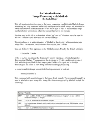
1. An Introduction to
Image Processing with MatLab
By: Rachel Hager
This lab is going to introduce you to the image processing capabilities in MatLab. Image
processing is a very important and widely used process in which images are processed to
retrieve information that is not visible to the naked eye, as well as it is used in a large
number of other applications where the standard picture is not enough.
The first step in this lab is to download all the ‘jpg’ and ‘tif’ files that are to be used in
this lab. You can locate them as a link on the webpage.
The second step is to set the directory of MatLab to the directory which contains your
image files. Be sure that you create this directory on your U-drive.
You can do this by first typing cd on the MatLab prompt. Usually the default setting is:
c:MatlabR12work
If this is so, you can change the directory by simply typing cd .. which changes the
directory to c:Matlab. You can repeat the step to go to C: drive and then type cd u:.
This will change the MatLab directory to your U-drive. Once you are in the right
directory you are all set to start doing some serious image processing.
In order to read the image we use the following command in MatLab
imread(‘filename’);
This command will save the image in the Image detail module. The command imread() is
used in MatLab to store image file. Image files that are supported by MatLab include the
following:

2. Since bitmap images are fairly large, they take a long time to convert into matrices.
Hence we stick to jpeg and tiff image formats in this lab.
This lab consists of 8 parts to help familiarize you with the basics of image processing:
1. Storing an Image
2. Creating the Negative of an Image
3. RGB Components of an Image
4. Gamma Scaling of an Image
5. Converting an Image to Grayscale
6. Creating a Histogram of an Image
7. Brightening an Image
8. Dithering an Image
1 Storing an Image
An image is stored in MatLab in the form of an image matrix. This matrix contains the
values of all the pixels in the image. In the case of a grayscale image, the image matrix is
a 2x2 matrix. In the case of a color image we have a 3x3 matrix.
Type the following command
Myimage = imread(‘filename’);
The filename should be complete. For example:
‘U:EE186LabsImageProcessingflowers.tiff’

3. If there were no errors, you stored the image correctly. If you see the error “Cannot find
file…” that means you either do not have the image saved in your directory, you have the
image name wrong, or you might be in the wrong directory.
After storing this image, you can view it using the command
imshow(Myimage);
The image will open in a new window.
2. Creating the Negative of an Image
In order to see the negative of the image, you will need to change the values in the image
matrix to double precision. This is done to invert the color matrix. The code below
negates the image:
negImage = double(Myimage); % Convert the image matrix to double
negImageScale = 1.0/max(negImage(:)); % Find the max value in this
% new array and take its
% inverse
negImage = 1 - negImage*negImageScale; % Multiply the double image
% matrix by the factor of
% negImageScale and subtract
% the total from 1
figure; % Draw the figure
imshow(negImage); % Show the new image
The above manipulations will result in a negative image that is exactly opposite in color
to the original image.
3. RGB Components of an Image
MatLab has the ability to find out exactly how much Red, Green, Blue content there is in
an image. You can find this out by selecting only one color at a time and viewing the
image in that color. The following code allows you to view the Red content of an image:
redimage = Myimage; % Create a new matrix equal to the matrix
% of your original image.
redimage (:, :, 2:3) = 0; % This selectively nullifies the second
% and third columns of the colormap
% matrix which are part of the original matrix. Since the colors
% are mapped using RGB, or columns with values of Red, Green and
% Blue, so we can selectively nullify the green and blue columns to
% obtain only the red part of the image.
imshow(redimage); % show the redimage that you just created.
Similarly, we can do the same with the green and blue components of the image. Just
keep in mind the format of the array
Red : Green : Blue
1 2 3

4. Try checking the blue component of the image. The only thing you will need to change is
the column numbers at the end of the statement.
blueimage = Myimage; % Create a new matrix equal to the matrix
% of your original image.
blueimage(:, :, 1:2) = 0; % Note the difference in column
% numbers.
imshow(blueimage); % Display the blueimage you just created.
Now try the green component yourself. There is a little trick to this.
After trying the green component of the image, try to see two components at a time. You
can do this by nullifying only one column at a time instead of two. (Hint: You only need
to put one number instead of 1:2 or 1:2:3 etc. Just write 1 or 2 or 3 to see the
combinations and note them.)
4. Gamma Scaling of an Image
Gamma scaling is an important concept in graphics and games. It relates to the pixel
intensities of the image. The format is simple:
J = imadjust(I, [low high], [bottom top], gamma);
This transforms the values in the intensity image I to values in J by mapping values
between low and high to values between bottom and top. Values below low and above
high are clipped. That is, values below low map to bottom, and those above high map to
top. You can use an empty matrix ([]) for [low high] or for [bottom top] to specify the
default of [0 1]. The variable gamma specifies the shape of the curve describing the
relationship between the values in I and J. If gamma is less than 1, the mapping is
weighted toward higher (brighter) output values. If gamma is greater than 1, the mapping
is weighted toward lower (darker) output values. If you omit the argument, gamma
defaults to 1 (linear mapping). Now try the following gamma variations and note down
the changes in intensities of the image.
NewImage = imadjust(Myimage, [.2, .7], []);
figure;
imshow(NewImage);
Note that the original image has gamma at default since there is no value of gamma
added. Now try this:
NewImage = imadjust(Myimage, [.2, .7], [], .2);
figure;
imshow(NewImage);
Note the difference? The gamma has been changed, so we see a change in the image
intensity. The intensity of each pixel in the image has increased. This clarifies the

5. explanation of gamma above. Now try a new value of gamma. This time use a value of 2
instead of .2.
Newimage = imadjust(x, [.2, .7], [], 2);
figure;
imshow(Newimage);
What happened? How did this change affect the gamma? Comment on your findings.
5. Converting an Image to Grayscale
MatLab allows us to change a color image into a grayscale image with ease. One way to
do this is to make all the values of the RGB components equal. MatLab provides a
function to do this.
Simply type the following:
grayimage = rgb2gray(Myimage);
figure;
imshow(grayimage);
The new image formed is in gray scale. The rgb2gray() function does exactly what it
says, changes the RGB image into gray; it basically forces all the RGB components to be
equal.
6. Brightening an Image
Another very useful and easy function that MatLab provides us is the function to brighten
an image. However, keep in mind that this function can be used only with the grayscale
images.
Simply type the following command after reading in the image, scaling it to gray, and
viewing it.
brighten(beta); % Set beta to any value between -1.0 and 1.0
We will see how to brighten a colored image in a later lab.
7. Creating a Histogram of an Image
An image histogram is a chart that shows the distribution of the different intensities in an
image. Each color level is represented, as a point on x-axis and on y-axis is the number of
instances of color level repetitions in the image. A histogram may be viewed with the
imhist() command. Sometimes all the important information in an image lies only in a
small region of colors, hence it is usually difficult to extract information from the image.
To balance the brightness level of an image, we carryout an image processing operation
termed histogram equalization.

6. In order to see the histogram of your favorite image use the following steps:
Myimage = imread('image'); % Read in your favorite image
figure; % Create figure to place image on
imshow(Myimage); % View the image
figure; % Create another figure for the histogram
imhist(Myimage); % Draw the histogram chart
[eqImage, T]=histeq(Myimage); % Equalize the image, that is
% equalize the intensity of the pixels
% of the image
figure; % Create another figure to place the image
imshow(eqImage); % Draw the equalized image
figure; % Create a figure for the histogram
imhist(eqImage); % Draw the equalized histogram
figure; % Create another figure to place a plot
plot((0:255)/255, T); % Plot the graph of the vector T
The vector T should contain integer counts for equally spaced bins with intensity values
in the appropriate range: [0, 1] for images of class double, [0, 255] for images of class
uint8, and [0, 65535] for images of class uint16.
8. Dither an Image
Dithering is a color reproduction technique in which dots or pixels are arranged in such a
way that allows us to perceive more colors than are actually used. This method of
"creating" a large color palette with a limited set of colors is often used in computer
images, television, and the printing industry. Images in MatLab can be dithered by using
the predefined functions. One easy way to do this is as follows:
figure('Name', 'Myimage - indexed, no dither');
[Myimagenodither, Myimagenodithermap]=rgb2ind(Myimage, 16, 'nodither');
imshow(Myimagenodither, Myimagenodithermap);
figure('Name', 'Myimage - indexed, dithered');
[Myimagedither, Myimagedithermap] = rgb2ind(Myimage, 16, 'dither');
imshow(Myimagedither, Myimagedithermap);
Type the above commands in the MatLab command prompt and check the images.
How do they differ? Do you feel one is better than the other? Which one seems a bit more
detailed? Comment on all your findings.
When finished, feel free to experiment, discover, learn and have fun….it is all about how
much you like to play and learning starts to happen as you have fun. Challenge yourself
and learn. Report and comment all of your finding.