BH curve hysteresis in ferro ferrimagnets

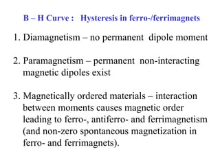
1. B – H Curve : Hysteresis in ferro-/ferrimagnets 1. Diamagnetism – no permanent dipole moment 2. Paramagnetism – permanent non-interacting magnetic dipoles exist 3. Magnetically ordered materials – interaction between moments causes magnetic order leading to ferro-, antiferro- and ferrimagnetism (and non-zero spontaneous magnetization in ferro- and ferrimagnets).

2. Types of magnetism 1. Diamagnetism Absence of Permanent magnetic moments  Fully filled orbitals On application of magnetic field (H), magnetic moment is induced in such a way to oppose the effect of H Occurs through distortion of orbitals It is proportional to the total no. of electrons . χ dia ~ 10 -6 and is independent of Temperature(T)

3. 2. Paramagnetism : Unpaired electrons existing in any orbital Permanent magnetic moments exist on atoms or ions Applied H orients the moments already present, against thermal agitation to randomize them Magnetization M = m/V ; i.e. M is magnetic moment per unit volume Magnetic Susceptibility:  ~ 10 -3  = M/H

4. Ferromagnetism : M is large M = Ng  B J B J (y) ; y = g  B H m /k B T Molecular field H m = H +  M,  is the Weiss molecular field constant B J (y) is the Brillouin function At high T,  = C/(T-  ) …Curie –Weiss Law At low T, large H : M saturates Induction B =  0 ( H+M) ; Permeability  = B/H Antiferromagnetism : M = 0,  = C/(T+  ) y

5. Magnetic order from T dependence of Susceptibility

6. Domain Theory- Competing Energies 1. Magnetostatic energy H d = -N d M ; E d = (  0 /2)N d M 2 N d is demagnetizing factor 2. Magnetocrystalline energy 3. Exchange Energy J =  S i .S J Minimization of total energy leads to formation of domains separated by domain walls. When H is applied, M develops due to movement of Domain walls Irreversible wall motion causes hysteresis and losses

7. Anisotropy energy : is due to preference of certain crystallographic directions for the alignment of atomic moments M vs. H for Fe ( Cubic) and Co (Hexagonal) Anisotropy constants Cubic : K Uniaxial : K 1 , K 2 E a = K 1 Sin 2  + K 2 Sin 4   : / M, EA

8. Domains and Domain walls 180 0 wall

10. Integrator C R2 R1 P s S s P S Variac Step down Transformer Circuit : V x (  H ) V Y (  B) Sample V x to X – plates of CRO V y to Y- plates of CRO One Primary and one secondary

11. Loop Tracer for Toroidal Sample Mutual Inductance set up One primary &Two secondaries – directly gives M – H loops Single primary and single secondary Emf 1 = - N S A µ 0  (H+M) /  t Emf 2 = - N S A µ 0  (H) /  t

12. Hysteresis loops Domain theory : Irreversible motion of domain walls causes hysteresis , large coercivity Presence of defects in domains, domain boundaries causes pinning of the walls & large hysteresis Barkhausen effect - Wall diplacement occurs by jerks

13. Barkhausen Effect Cilcks can be heard on a loud speaker Domain walls need to cross potential wells in the magnetization process Flexible Domain Wall - Contributes to Reversible M

14. Steps during Magnetization Process H = 0, Random directions of domains Low fields,Reversible Easy dirns. Close to H expand Medium fields, Domains in other equivalent Easy dirns. High fields Domain rotation to H dirn .

15. H = 0 Low H Medium H High H

16. Formulae : 1. Magnetic field H = n p I in (A/m) ; I = V R /R Here n p = N p /l p - i.e.no. of turns in primary per unit length. N p is the no. of turns in the Primary a) Solenoid : l p = length of primary b) Toroid : l p = 2  r , where r = (r 1 +r 2 ) / 2 r 2 r 1 1 kA/m = 4  Oe,1 Tesla /  0 = 1 A/m 1 T = 10 4 Oe ;  0 = 4  * 10 -7 H / m Toroid

18.  where  = 2  f where f is the frequency of ac signal used. Here f = 50 Hz ( the line frequency) Secondary Output Let B = B 0 Sin  t

19. C R 2 R 1 1. To determine the calibration constant of Integrator 2. Measure the value of R in the primary circuit to determine current I, I = V R /R

20. Calculate remanance ( B r ), coercivity ( H c ), saturation magnetization ( M s ), field required for saturation ( H s ), Saturation Induction ( B s ) = 4  M s AC Hysteresis loss (W) from the measured B-H curves. The ((1/4  )*area under the B-H curve) gives the information about hysteresis loss in CGS units ( erg / cc / cycle )

21. Corrections 1. Demagnetisation The rod shaped ( l / d > 10) and Toroidal shaped samples are chosen to minimize the demagnetizing factors (N) so that H int = H / (1-N)  H is a valid approximation. 2. Filling Factor : Here, the sample is assumed to fill the volume of the secondary coil completely. If not, we introduce a Filling Factor (  ) correction which defines the extent of sample filling in the secondary coil.