Financial risk management

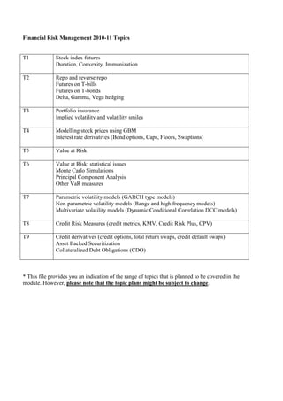
Financial Risk Management 2010-11 Topics

T1 Stock index futures
Duration, Convexity, Immunization

T2 Repo and reverse repo
Futures on T-bills
Futures on T-bonds
Delta, Gamma, Vega hedging

T3 Portfolio insurance
Implied volatility and volatility smiles

T4 Modelling stock prices using GBM
Interest rate derivatives (Bond options, Caps, Floors, Swaptions)

T5 Value at Risk

T6 Value at Risk: statistical issues
Monte Carlo Simulations
Principal Component Analysis
Other VaR measures

T7 Parametric volatility models (GARCH type models)
Non-parametric volatility models (Range and high frequency models)
Multivariate volatility models (Dynamic Conditional Correlation DCC models)

T8 Credit Risk Measures (credit metrics, KMV, Credit Risk Plus, CPV)

T9 Credit derivatives (credit options, total return swaps, credit default swaps)
Asset Backed Securitization
Collateralized Debt Obligations (CDO)

* This file provides you an indication of the range of topics that is planned to be covered in the
module. However, please note that the topic plans might be subject to change.

Topics
Financial Risk Management Futures Contract:
Speculation, arbitrage, and hedging
Topic 1
Stock Index Futures Contract:
Managing risk using Futures
Reading: CN(2001) chapter 3 Hedging (minimum variance hedge
ratio)
Hedging market risks

Futures Contract
Agreement to buy or sell “something” in the future at
a price agreed today. (It provides Leverage.)
Speculation with Futures: Buy low, sell high
Futures (unlike Forwards) can be closed anytime by taking
an opposite position
Speculation with Futures
Arbitrage with Futures: Spot and Futures are linked
by actions of arbitragers. So they move one for one.
Hedging with Futures: Example: In January, a farmer
wants to lock in the sale price of his hogs which will
be “fat and pretty” in September.
Sell live hog Futures contract in Jan with maturity in Sept

Speculation with Futures Speculation with Futures
Purchase at F0 = 100
Hope to sell at higher price later F1 = 110
Profit/Loss per contract
Close-out position before delivery date. Long future
Obtain Leverage (i.e. initial margin is ‘low’) $10

Example:
Example: Nick Leeson: Feb 1995 F1 = 90
0

F0 = 100
Long 61,000 Nikkei-225 index futures (underlying F1 = 110 Futures price
value = $7bn).
-$10
Nikkei fell and he lost money (lots of it)
- he was supposed to be doing riskless ‘index Short future
arbitrage’ not speculating

Speculation with Futures
Profit payoff (direction vectors)
F increase F increase
then profit increases then profit decrease

Profit/Loss Profit/Loss
Arbitrage with Futures
-1
+1
Underlying,S
+1 or Futures, F -1

Long Futures Short Futures
or, Long Spot or, Short Spot

Arbitrage with Futures Arbitrage with Futures
At expiry (T), FT = ST . Else we can make riskless General formula for non-income paying security:
profit (Arbitrage). F0 = S0erT or F0 = S0(1+r)T
Forward price approaches spot price at maturity
Futures price = spot price + cost of carry
Forward price, F
Forward price ‘at a premium’ when : F > S (contango)
For stock paying dividends, we reduce the ‘cost of
carry’ by amount of dividend payments (d)
F0 = S0e(r-d)T
0 Stock price, St
T
At T, ST = FT For commodity futures, storage costs (v or V) is
negative income
Forward price ‘at a discount’, when : F < S (backwardation)
F0 = S0e(r+v)T or F0 = (S0+V)erT

Arbitrage with Futures Arbitrage with Futures
For currency futures, the ‘cost of carry’ will be Arbitrage at t<T for a non-income paying security:
reduced by the riskless rate of the foreign currency If F0 > S0erT then buy the asset and short the futures
contract
(rf)
If F0 < S0erT then short the asset and buy the futures
F0 = S0e(r-rf)T
contract

For stock index futures, the cost of carry will be Example of ‘Cash and Carry’ arbitrage: S=£100,
reduced by the dividend yield r=4%p.a., F=£102 for delivery in 3 months.
0.04×0.25
F0 = S0e(r-d)T We see F = 100 × e
ɶ = 101 £
Since Futures is over priced,
time = Now time = in 3 months
•Sell Futures contract at £102 •Pay loan back (£101)
•Borrow £100 for 3 months and buy stock •Deliver stock and get agreed price of £102

Hedging with Futures
F and S are positively correlated
To hedge, we need a negative correlation. So we
long one and short the other.
Hedging with Futures Hedge = long underlying + short Futures

Hedging with Futures Hedging with Futures
Simple Hedging Example: F1 value would have been different if r had changed.
You long a stock and you fear falling prices over the This is Basis Risk (b1 = S1 – F1)
next 2 months, when you want to sell. Today (say
January), you observe S0=£100 and F0=£101 for Final Value = S1 + (F0 - F1 ) = £100.7
April delivery. = (S1 - F1 ) + F0
so r is 4% = b1 + F0
Today: you sell one futures contract
In March: say prices fell to £90 (S1=£90). So where “Final basis” b1 = S1 - F1
F1=S1e0.04x(1/12)=£90.3. You close out on Futures.
At maturity of the futures contract the basis is zero
Profit on Futures: 101 – 90.3 = £10.7
(since S1 = F1 ). In general, when contract is closed
Loss on stock value: 100 – 90 =£10
out prior to maturity b1 = S1 - F1 may not be zero.
Net Position is +0.7 profit. Value of hedged portfolio However, b1 will usually be small in relation to F0.
= S1+ (F0 - F1) = 90 + 10.7 = 100.7

Stock Index Futures Contract
Stock Index Futures contract can be used to
eliminate market risk from a portfolio of stocks
F0 = S0 × e( r − d )T
If this equality does not hold then index arbitrage
Stock Index Futures Contract (program trading) would generate riskless profits.

Risk free rate is usually greater than dividend yield
Hedging with SIFs (r>d) so F>S

Hedging with Stock Index Futures Hedging with Stock Index Futures
Example: A portfolio manager wishes to hedge her The required number of Stock Index Futures contract
portfolio of $1.4m held in diversified equity and to short will be 3
S&P500 index  TVS 0   $1, 400, 000 
Total value of spot position, TVS0=$1.4m NF = −  = −  = − 3.73
S0 = 1400 index point  FVF0   $375, 000 
Number of stocks, Ns = TVS0/S0 = $1.4m/1400 In the above example, we have assumed that S and
=1000 units F have correlation +1 (i.e. ∆ S = ∆ F )
We want to hedge Δ(TVSt)= Ns . Δ(St)
In reality this is not the case and so we need
Use Stock Index Futures, F0=1500 index point, z= minimum variance hedge ratio
contract multiplier = $250
FVF0 = z F0 = $250 ( 1500 ) = $375,000

Minimum Variance Hedge Ratio To obtain minimum, we differentiate with respect to Nf
2
∆V = change in spot market position + change in Index Futures position (∂σ V / ∂N f = 0 ) and set to zero
= Ns . (S1-S0) + Nf . (F1 - F0) z
= Ns S0. ∆S /S0 + ∆
Nf F0. (∆F /F0) z N f ( F V F0 ) 2 σ ∆ F / F
2
= −TVS
0
⋅ F V F ⋅ σ ∆ S / S ,∆ F / F
0
= TVS0 . ∆S /S0 + ∆
Nf . FVF0 . (∆F /F0)
 TVS0 
where, z = contract multiple for futures ($250 for S&P 500 Futures); ∆S = N f = −   ( σ ∆ S / S ,∆ F / F 2
σ ∆F / F )
S1 - S0, ∆F = F1 - F0  F V F0 
 TVS0 
=−  β ∆ S / S ,∆ F / F
The variance of the hedged portfolio is
2 2 2 2
σ V = (TVS 0 ) σ ∆S / S + ( N f ) ( FVF ) σ ∆F / F
2 2  F V F0 
0 where Ns = TVS0/S0 and beta is regression coefficient of the
+ 2N TVS 0 FVF0 . σ ∆S / S , ∆F / F regression
f (∆S / S ) = α 0 + β ∆S / ∆F ( ∆ F / F ) + ε

SUMMARY 2 Application: Changing beta of your portfolio: “Market
∂σV / ∂N = 0 implies Timing Strategy”
f TVS
Nf = 0
.( β h − β p )
TVS 0 FVF0
Nf = − .β p Example: βp (=say 0.8) is your current ‘spot/cash’ portfolio of stocks
FVF0 But

 Value of Spot Position 
= −
 FaceValue of futures at t = 0 



βp • You are more optimistic about ‘bull market’ and desire a higher exposure of
βh (=say, 1.3)
• It’s ‘expensive’ to sell low-beta shares and purchase high-beta shares
If correlation = 1, the beta will be 1 and we just have • Instead ‘go long’ more Nf Stock Index Futures contracts
TVS0
Nf = − Note: If βh= 0, then Nf = - (TVS0 / FVF0) βp
FVF0

Application: Stock Picking and hedging market risk
If you hold stock portfolio, selling futures will place a
You hold (or purchase) 1000 undervalued shares of Sven plc
hedge and reduce the beta of your stock portfolio.
If you want to increase your portfolio beta, go long V(Sven) = $110 (e.g. Using Gordon Growth model)
futures.
P(Sven) = $100 (say)
Example: Suppose β = 0.8 and Nf = -6 contracts would
make β = 0. Sven plc are underpriced by 10%.

If you short 3 (-3) contracts instead, then β = 0.4 Therefore you believe Sven will rise 10% more than the market over the next
3 months.
If you long 3 (+3) contracts instead, then β = 0.8+0.4
= 1.2 But you also think that the market as a whole may fall by 3%.

The beta of Sven plc (when regressed with the market return) is 2.0

Can you ‘protect’ yourself against the general fall in the market and hence any Application: Future stock purchase and hedging market
‘knock on’ effect on Sven plc ? risk
Yes . Sell Nf index futures, using: You want to purchase 1000 stocks of takeover target with βp = 2, in 1
month’s time when you will have the cash.
TVS
N f = − 0
.β p
You fear a general rise in stock prices.
FVF 0 Go long Stock Index Futures (SIF) contracts, so that gain on the futures will
offset the higher cost of these particular shares in 1 month’s time.
If the market falls 3% then TVS
N f = 0
.β p
Sven plc will only change by about 10% - (2x3%) = +4% FVF 0

SIF will protect you from market risk (ie. General rise in prices) but not from
But the profit from the short position in Nf index futures, will give you an specific risk. For example if the information that you are trying to takeover
additional return of around 6%, making your total return around 10%. the firm ‘leaks out’ , then price of ‘takeover target’ will move more than that
given by its ‘beta’ (i.e. the futures only hedges market risk)

Topics
Financial Risk Management Duration, immunization, convexity
Repo (Sale and Repurchase agreement)
Topic 2 and Reverse Repo
Managing interest rate risks
Reference: Hull(2009), Luenberger (1997), and CN(2001)
Hedging using interest rate Futures
Futures on T-bills
Futures on T-bonds

Readings
Books
Hull(2009) chapters 6
CN(2001) chapters 5, 6
Luenberger (1997) chapters 3
Journal Article Hedging Interest rate risks: Duration
Fooladi, I and Roberts, G (2000) “Risk Management with Duration Analysis”
Managerial Finance,Vol 25, no. 3

Duration Duration (also called Macaulay Duration)
Duration measures sensitivity of price changes (volatility) with Duration of the bond is a measure that summarizes
changes in interest rates approximate response of bond prices to change in yields.
1 Lower the coupons A better approximation could be convexity of the bond .
T for a given time to n

PB = ∑ C t t + ParValueT maturity, greater B = ∑ c i e − y ti
(1+ r )
weight
t =1 (1+ r )
T change in price to i =1
change in interest n
rates
∑ t i ⋅ c i e − y ti n
 c e − y ti 
T
2 Greater the time to D = i =1
= ∑ ti  i 
PB = ∑ C t t + ParValueT
maturity with a given B i =1  B 
coupon, greater
t =1 (1+ r ) (1+ r )
T
change in price to Duration is weighted average of the times when payments
change in interest are made. The weight is equal to proportion of bond’s total
rates present value received in cash flow at time ti.
3 For a given percentage change in yield, the actual price increase is Duration is “how long” bondholder has to wait for cash flows
greater than a price decrease

Macaulay Duration Modified Duration and Dollar Duration
For a small change in yields ∆ y / d y For Macaulay Duration, y is expressed in continuous
compounding.
dB
∆B = ∆y When we have discrete compounding, we have Modified
dy Duration (with these small modifications)
Evaluating d B :  n
 If y is expressed as compounding m times a year, we divide D
d y ∆ B =  − ∑ t i c i e − y ti  ∆ y by (1+y/m) ∆B = − B ⋅ D
 i =1  ⋅ ∆y
(1 + y / m)
= −B ⋅ D ⋅∆y
∆B = − B ⋅ D* ⋅ ∆y
∆B
= −D ⋅∆y
B Dollar Duration, D$ = B.D
D measures sensitivity of percentage change in bond That is, D$ = Bond Price x Duration (Macaulay or Modified)
prices to (small) changes in yields ∆B = − D$ ⋅ ∆y
∆B
Note negative relationship between Price (B) So D$ is like Options Delta D$ = −
∆y
and yields (Y)

Duration Duration -example
Example: Consider a trader who has $1 million in Example: Consider a 7% bond with 3 years to maturity. Assume that the bond
is selling at 8% yield.
bond with modified duration of 5. This means for
A B C D E
every 1 bp (i.e. 0.01%) change in yield, the value of
the bond portfolio will change by $500. Present value Weight =
Year Payment Discount A× E
∆B = − ( $1, 000, 000 × 5 ) ⋅ 0.01% = −$500 =B× C D/Price
factor 8%
A zero coupon bond with maturity of n years has a 0.5 3.5 0.962 3.365 0.035 0.017
Duration = n 1.0 3.5 0.925 3.236 0.033 0.033
A coupon-bearing bond with maturity of n years will 1.5 3.5 0.889 3.111 0.032 0.048
have Duration < n 2.0 3.5 0.855 2.992 0.031 0.061
2.5 3.5 0.822 2.877 0.030 0.074
Duration of a bond portfolio is weighted average of
3.0 103.5 0.79 81.798 0.840 2.520
the durations of individual bonds Sum Price = 97.379 Duration = 2.753
D p o r tfo lio = ∑ (B
i
i / B )⋅ D i
Here, yield to maturity = 0.08, m = 2, y = 0.04, n = 6, Face value = 100.

Qualitative properties of duration Properties of duration
Duration of bonds with 5% yield as a function of
maturity and coupon rate. 1. Duration of a coupon paying bond is always less
than its maturity. Duration decreases with the increase
Coupon rate of coupon rate. Duration equals bond maturity for non-
Years to 1% 2% 5% 10% coupon paying bond.
maturity
1 0.997 0.995 0.988 0.977 2. As the time to maturity increases to infinity, the
2 1.984 1.969 1.928 1.868
5 4.875 4.763 4.485 4.156
duration do not increase to infinity but tend to a finite
10 9.416 8.950 7.989 7.107 limit independent of the coupon rate.
25 20.164 17.715 14.536 12.754
50 26.666 22.284 18.765 17.384 1+ m
λ
Actually, D → where λ is the yield to maturity
100 22.572 21.200 20.363 20.067 λ
Infinity 20.500 20.500 20.500 20.500 per annum, and m is the number of coupon
payments per year.

Properties of Duration Changing Portfolio Duration

3. Durations are not quite sensitive to increase in Changing Duration of your portfolio:
coupon rate (for bonds with fixed yield). They don’t If prices are rising (yields are falling), a bond
vary huge amount since yield is held constant and
trader might want to switch from shorter
it cancels out the influence of coupons.
duration bonds to longer duration bonds as
4. When the coupon rate is lower than the yield, the longer duration bonds have larger price
duration first increases with maturity to some changes.
maximum value then decreases to the asymptotic
limit value. Alternatively, you can leverage shorter
maturities. Effective portfolio duration =
5. Very long durations can be achieved by bonds with ordinary duration x leverage ratio.
very long maturities and very low coupons.

Immunization (or Duration matching) Immunization
This is widely implemented by Fixed Income Practitioners. Matching present values (PV) of portfolio and obligations
This means that you will meet your obligations with the cash
time 0 time 1 time 2 time 3 from the portfolio.
If yields don’t change, then you are fine.
0 pay $ pay $ pay $ If yields change, then the portfolio value and PV will both change
You want to safeguard against interest rate increases. by varied amounts. So we match also Duration (interest rate risk)
A few ideas: PV1 + PV2 = PVobligation
1. Buy zero coupon bond with maturities matching timing of Matching duration
cash flows (*Not available) [Rolling hedge has reinv. risk] Here both portfolio and obligations have the same sensitivity to
interest rate changes.
2. Keep portfolio of assets and sell parts of it when cash is
needed & reinvest in more assets when surplus (* difficult as If yields increase then PV of portfolio will decrease (so will the PV
of the obligation streams)
Δ value of in portfolio and Δ value of obligations will not
identical) If yields decrease then PV of portfolio will increase (so will the PV
of the obligation streams)
3. Immunization - matching duration and present values D1 PV1 + D 2 PV2 = Dobligation PVobligation
of portfolio and obligations (*YES)

Immunization Immunization
Example Suppose only the following bonds are available for its choice.
coupon rate maturity price yield duration
Suppose Company A has an obligation to Bond 1 6% 30 yr 69.04 9% 11.44
pay $1 million in 10 years. How to invest Bond 2 11% 10 yr 113.01 9% 6.54
in bonds now so as to meet the future Bond 3 9% 20 yr 100.00 9% 9.61

obligation? • Present value of obligation at 9% yield is $414,642.86.

• An obvious solution is the purchase of a • Since Bonds 2 and 3 have durations shorter than 10 years, it is not
simple zero-coupon bond with maturity 10 possible to attain a portfolio with duration 10 years using these
two bonds.
years.
Suppose we use Bond 1 and Bond 2 of amounts V1 & V2,
* This example is from Leunberger (1998) page 64-65. The numbers V1 + V2 = PV
are rounded up by the author so replication would give different P1V1 + D2V2 = 10 × PV
numbers.
giving V1 = $292,788.64, V2 = $121,854.78.

Immunization Immunization
Yield
9.0 8.0 10.0
Bond 1
Difficulties with immunization procedure
Price 69.04 77.38 62.14 1. It is necessary to rebalance or re-immunize the
Shares 4241 4241 4241 portfolio from time to time since the duration depends
Value 292798.64 328168.58 263535.74 on yield.
Bond 2 2. The immunization method assumes that all yields
Price 113.01 120.39 106.23 are equal (not quite realistic to have bonds with
Shares 1078 1078 1078 different maturities to have the same yield).
Value 121824.78 129780.42 114515.94
Obligation 3. When the prevailing interest rate changes, it is
value 414642.86 456386.95 376889.48 unlikely that the yields on all bonds change by the
Surplus -19.44 1562.05 1162.20 same amount.
Observation: At different yields (8% and 10%), the value of the
portfolio almost agrees with that of the obligation.

Duration for term structure Duration for term structure
We want to measure sensitivity to parallel shifts in the spot
rate curve
Consider parallel shift in term structure: sti changes to sti + ∆y ( )
Then PV becomes
For continuous compounding, duration is called Fisher-Weil
Fisher- n
( )
P ( ∆y ) =
− sti + ∆ y ⋅ti
duration.
duration ∑x
i=0
ti ⋅e
If x0, x1,…, xn is cash flow sequence and spot curve is st where
t = t0,…,tn then present value of cash flow is Taking differential w.r.t ∆y in the point ∆y=0 we get
n
dP ( ∆ y ) n

∑x
− sti ⋅ti
| ∆ y = 0 = − ∑ t i x t i ⋅ e ti i
− s ⋅t
PV = ⋅e
d ∆y
ti
i=0 i=0

The Fisher-Weil duration is So we find relative price sensitivity is given by DFW
n
1 1 dP (0)
∑t
− sti ⋅ti
D FW = ⋅ x ti ⋅ e ⋅ = − D FW
PV i=0
i
P (0) d ∆ y

Convexity Convexity
Duration applies to only small changes in y Convexity for a bond is
n
Two bonds with same duration can have different
1 d 2B ∑ t i2 ⋅ c i e − y t i n
 c e − y ti 
change in value of their portfolio (for large changes C =
B dy 2
= i =1

B
= ∑ t i2  i 
in yields) i =1  B 
Convexity is the weighted average of the ‘times squared’
when payments are made.
From Taylor series expansion
dB 1 d 2B
∆ B = ∆ y + (∆ )
2
y
dy 2 dy 2
∆ B 1
= − D ⋅ ∆ y + C ⋅ (∆ )
2
y
B 2
First order approximation cannot capture this, so we
So Dollar convexity is like Gamma measure in
take second order approximation (convexity)
options.

Short term risk management using Repo
Repo is where a security is sold with agreement to buy it back at
a later date (at the price agreed now)
Difference in prices is the interest earned (called repo rate
rate)
It is form of collateralized short term borrowing (mostly overnight)
Example: a trader buys a bond and repo it overnight. The
REPO and REVERSE REPO money from repo is used to pay for the bond. The cost of this
deal is repo rate but trader may earn increase in bond prices
and any coupon payments on the bond.

There is credit risk of the borrower. Lender may ask for
margin costs (called haircut) to provide default protection.
Example: A 1% haircut would mean only 99% of the value of
collateral is lend in cash. Additional ‘margin calls’ are made if
market value of collateral falls below some level.

Short term risk management using Repo
Hedge funds usually speculate on bond price differentials
using REPO and REVERSE REPO
Example: Assume two bonds A and B with different prices (say price(A)<price(B)) but
similar characteristics. Hedge Fund (HF) would like to buy A and sell B
simultaneously.This can be financed with repo as follows:
(Long position) Buy Bond A and repo it. The cash obtained is used to pay for Interest Rate Futures
the bond. At repo termination date, sell the bond and with the cash buy
bond back (simultaneously). HF would benefit from the price increase in
bond and low repo rate (Futures on T-Bills)
(short position) Enter into reverse repo by borrowing the Bond B (as
collateral for money lend) and simultaneously sell Bond B in the market. At
repo termination date, buy bond back and get your loan back (+ repo
rate). HF would benefit from the high repo rate and a decrease in price of
the bond.

Interest Rate Futures Interest Rate Futures
In this section we will look at how Futures contract written on a
Treasury Bill (T-Bill) help in hedging interest rate risks So what is a 3-month T-Bill Futures contract?
At expiry, (T), which may be in say 2 months time
Review - What is T-Bill?
the (long) futures delivers a T-Bill which matures at
T-Bills are issued by government, and quoted at a discount
T+90 days, with face value M=$100.
Prices are quoted using a discount rate (interest earned as % of
face value) As we shall see, this allows you to ‘lock in’ at t=0, the forward
Example: 90-day T-Bill is quoted at 0.08 This means annualized
0.08. rate, f12
return is 8% of FV. So we can work out the price, as we know FV. T-Bill Futures prices are quoted in terms of quoted index, Q
  d   90  (unlike discount rate for underlying)
P = F V 1 −   
  100   360  Q = $100 – futures discount rate (df)
Day Counts convention (in US)
So we can work out the price as
1. Actual/Actual (for treasury bonds)
  d f   90 
2. 30/360 (for corporate and municipal bonds) F = F V 1 −   
3. Actual/360 (for other instruments such as LIBOR)   100   360 

Hedge decisions Cross Hedge: US T-Bill Futures
Example:
When do we use these futures contract to hedge?
Today is May. Funds of $1m will be available in August to
Examples: invest for further 6 months in bank deposit (or commercial bills)
1) You hold 3m T-Bills to sell in 1-month’s time ~ fear price fall ~ spot asset is a 6-month interest rate
~ sell/short T-Bill futures Fear a fall in spot interest rates before August, so today BUY T-
bill futures
2) You will receive $10m in 3m time and wish to place it on a Eurodollar bank
deposit for 90 days ~ fear a fall in interest rates Assume parallel shift in the yield curve. (Hence all interest rates
~ go long a Eurodollar futures contract move by the same amount.)
~ BUT the futures price will move less than the price of the
3) Have to issue $100m of 180-day Commercial Paper in 3 months time (I.e. commercial bill - this is duration at work! higher the maturity, more
borrow money) ~ fear a rise in interest rates sensitive are changes in
~ sell/short a T-bill futures contract as there is no commercial bill futures prices to interest rates
contract (cross hedge) Use Sept ‘3m T-bill’ Futures, ‘nearby’ contract
~ underlying this futures contract is a 3-month interest rate

Cross Hedge: US T-Bill Futures Cross Hedge: US T-Bill Futures
Question: How many T-bill futures contract should I purchase?
3 month Desired investment/protection
exposure period period = 6-months We should take into account the fact that:
1. to hedge exposure of 3 months, we have used T-bill futures
with 4 months time-to-maturity
May Aug. Sept. Dec. Feb.
2. the Futures and spot prices may not move one-to-one
Maturity of ‘Underlying’ We could use the minimum variance hedge ratio:
in Futures contract
TVS0
Nf = .β p
FVF0
Purchase T-Bill Known $1m Maturity date of Sept.
future with Sept. cash receipts T-Bill futures contract
However, we can link price changes to interest rate
delivery date changes using Duration based hedge ratio

Duration based hedge ratio Duration based hedge ratio
Using duration formulae for spot rates and futures: Expressing Beta in terms of Duration:
∆S ∆F  TVS0 
= − DS ⋅ ∆ys = − DF ⋅ ∆yF Nf =   .β p
S F  FVF0 
We can obtain
So we can say volatility is proportional to Duration:  ∆S ∆F  last term by
Cov  , 
 ∆S   ∆F   TVS0   S F  regressing
σ2  = DS ⋅ σ ( ∆ys ) σ2  = DF ⋅ σ ( ∆yF ) =
2 2 2 2
 ∆yS = α0 + βy∆yF + ε
 S   F   FVF0  σ 2  ∆F 
 
 ∆S ∆F   F 
Cov  ,  = Ε ( − DS ⋅ ∆ys )( − DF ⋅ ∆yF ) 
 S F 
   TVS0  Ds  σ ( ∆ys ∆yF ) 
=   
= DS ⋅ DF ⋅ σ ( ∆ys ∆yF ) FVF0  DF  σ 2 ( ∆yF ) 
  

Duration based hedge ratio Cross Hedge: US T-Bill Futures
Example
Summary: REVISITED
3 month Desired investment/protection
 TVS0   Ds 
Nf = .  βy  exposure period period = 6-months

 FVF0   DF 
May Aug. Sept. Dec. Feb.
where beta is obtained from the regression of yields

∆yS = α0 + β y ∆yF + ε Maturity of ‘Underlying’
in Futures contract

Purchase T-Bill Known $1m Maturity date of Sept.
future with Sept. cash receipts T-Bill futures contract
delivery date

Cross Hedge: US T-Bill Futures Cross Hedge: US T-Bill Futures
Suppose now we are in August:
May (Today). Funds of $1m accrue in August to be invested for 6- months
3 month US T-Bill Futures : Sept Maturity
in bank deposit or commercial bills( Ds = 6 )
Spot Market(May) CME Index Futures Price, F Face Value of $1m
Use Sept ‘3m T-bill’ Futures ‘nearby’ contract ( DF = 3) (T-Bill yields) Quote Qf (per $100) Contract, FVF

May y0 (6m) = 11% Qf,0 = 89.2 97.30 $973,000
Cross-hedge.
August y1(6m) = 9.6% Qf,1 = 90.3 97.58 $975,750
Here assume parallel shift in the yield curve Change -1.4% 1.10 (110 ticks) 0.28 $2,750
(per contract)

Qf = 89.2 (per $100 nominal) hence: Durations are : Ds = 0.5, Df = 0.25
Amount to be hedged = $1m. No. of contracts held = 2
F0 = 100 – (10.8 / 4) = 97.30
F

FVF0 = $1m (F0/100) = $973,000 Key figure is F1 = 97.575 (rounded 97.58)
Gain on the futures position
Nf = (TVS0 / FVF0) (Ds / DF ) = TVS0 (F1 - F0) NF = $1m (0.97575 – 0.973) 2 = $5,500
= ($1m / 973,000) ( 0.5 / 0.25) = 2.05 (=2)

Cross Hedge: US T-Bill Futures
Invest this profit of $5500 for 6 months (Aug-Feb) at y1=9.6%:
= $5500 + (0.096/2) = $5764

Loss of interest in 6-month spot market (y0=11%, y1=9.6%)
= $1m x [0.11 – 0.096] x (1/2) = $7000 Interest Rate Futures
Net Loss on hedged position $7000 - $5764 = $1236
(so the company lost $1236 than $7000 without the hedge)
(Futures on T-Bonds)
Potential Problems with this hedge:
1. Margin calls may be required
2. Nearby contracts may be maturing before September. So we may have to roll
over the hedge
3. Cross hedge instrument may have different driving factors of risk

US T-Bond Futures US T-Bond Futures
Contract specifications of US T-Bond Futures at CBOT: Conversion Factor (CF): CF adjusts price of actual bond to be
(CF):
Contract size $100,000 nominal, notional US Treasury bond with 8% coupon delivered by assuming it has a 8% yield (matching the bond to
Delivery months March, June, September, December the notional bond specified in the futures contract)
Quotation Per $100 nominal Price = (most recent settlement price x CF) + accrued interest
Tick size (value) 1/32 ($31.25)
Last trading day 7 working days prior to last business day in expiry month
Example: Possible bond for delivery is a 10% coupon (semi-
Delivery day Any business day in delivery month (seller’s choice)
annual) T-bond with maturity 20 years.
Settlement Any US Treasury bond maturing at least 15 years from the
contract month (or not callable for 15 years) The theoretical price (say, r=8%):
40
5 100
Notional is 8% coupon bond. However, Short can choose to P=∑ i
+ = 119.794
deliver any other bond. So Conversion Factor adjusts “delivery i =1 1.04 1.0440
price” to reflect type of bond delivered Dividing by Face Value, CF = 119.794/100 = 1.19794 (per
T-bond must have at least 15 years time-to-maturity $100 nominal) If Coupon rate > 8% then CF>1
Quote ‘98-14’ means 98.(14/32)=$98.4375 per $100 nominal
‘98- If Coupon rate < 8% then CF<1

US T-Bond Futures Hedging using US T-Bond Futures
deliver:
Cheapest to deliver: Hedging is the same as in the case of T-bill Futures (except
In the maturity month, Short party can choose to deliver any Conversion Factor).
bond from the existing bonds with varying coupons and
maturity. So the short party delivers the cheapest one. For long T-bond Futures, duration based hedge ratio is given
by:
Short receives:
 TVS0   Ds 
(most recent settlement price x CF) + accrued interest Nf =  . β y  ⋅ CFCTD
Cost of purchasing the bond is:
 FVF0   DF 
Quoted bond price + accrued interest where we have an additional term for conversion factor for
the cheapest to deliver bond.
The cheapest to deliver bond is the one with the smallest:
Quoted bond price - (most recent settlement price x CF)

Financial Risk Management

Topic 3a
Managing risk using Options
Readings: CN(2001) chapters 9, 13; Hull Chapter 17

Topics

Financial Engineering with Options
Black Scholes
Delta, Gamma, Vega Hedging
Portfolio Insurance

Options Contract - Review
An option (not an obligation), American and European

-

Put Premium

-

Financial Engineering with options
Synthetic call option

Put-Call Parity: P + S = C + Cash
Example: Pension Fund wants to hedge its stock holding
against falling stock prices (over the next 6 months) and
wishes to temporarily establish a “floor value” (=K) but also
wants to benefit from any stock price rises.

Financial Engineering with options
Nick Leeson’s short straddle

You are initially credited with the call and put premia C + P (at t=0) but if at expiry
there is either a large fall or a large rise in S (relative to the strike price K ) then you
will make a loss
(.eg. Leeson’s short straddle: Kobe Earthquake which led to a fall in S
(S = “Nikkei-225”) and thus large losses).

Black Scholes
BS formula for price of European Call option d1 − σ
d 2 =D2=d1 T
− rT
c = S 0 N (d 1 ) − K e N (d 2 )

Probability of call option being in-the-money and getting stock

Present value of the strike price

Probability of exercise and paying strike price

c expected (average) value of receiving the stock in the event of
=
exercise MINUS cost of paying the strike price in the event of exercise

Black Scholes
where S   σ2  S   σ2 
ln  0 +r +  T ln  0 +r − T
K   2  ;d =  K   2 
d1 = or d 2 = d1 − σ T
σ T σ T
2

Sensitivity of option prices
Sensitivity of option prices (American/European non- non-
dividend paying)
c = f ( K, S0, r, T, σ ) This however can be negative for
- + ++ + dividend paying European options.
Example: stock pays dividend in
2 weeks. European call with 1
p = f ( K, S0, r, T, σ ) week to expiration will have more
+ - - + + value than European call with 3
weeks to maturity.

Call premium increases as stock price increases (but less than
one-for-one)
Put premium falls as stock price increases (but less than one-
for-one)

The Greek Letters
Delta, ∆ measures option price change when stock
price increase by $1
Gamma, Γ measures change in Delta when stock
price increase by $1
Vega, υ measures change in option price when there
is an increase in volatility of 1%
Theta, Θ measures change in option price when
there is a decrease in the time to maturity by 1 day
Rho, ρ measures change in option price when there
is an increase in interest rate of 1% (100 bp)

∂f ∂2 f ∂f ∂f ∂f
∆ = ;Γ = ;υ = ;Θ = ;ρ =
∂S ∂S 2
∂σ ∂T ∂r
Using Taylor series,

1
df ≈ ∆ ⋅dS + Γ ⋅ (d S ) + Θ ⋅dt + ρ ⋅dr + υ ⋅dσ
2

2

Read chapter 12 of McDonald text book “Derivative Markets” for more about Greeks

Delta
The rate of change of the option price with respect
to the share price
e.g. Delta of a call option is 0.6
Stock price changes by a small amount, then the option
price changes by about 60% of that

Option
price

Slope = ∆ = ∂c/ ∂ S
C

S Stock price

Delta
∆ of a stock = 1
∂C
∆ call = = N ( d1 ) > 0
∂S (for long positions)
∂P
∆ put = = N ( d1 ) − 1 < 0
∂S
If we have lots of options (on same underlying) then
delta of portfolio is
∆ portfolio = ∑ N k ⋅ ∆ k
k
where Nk is the number of options held. Nk > 0 if long
Call/Put and Nk < 0 if short Call/Put

Delta
So if we use delta hedging for a short call position, we
must keep a long position of N(d1) shares
What about put options?
The higher the call’s delta, the more likely it is that the
option ends up in the money:
Deep out-of-the-money: Δ ≈ 0
At-the-money: Δ ≈ 0.5
In-the-money: Δ≈1
Intuition: if the trader had written deep OTM calls, it
would not take so many shares to hedge - unlikely the
calls would end up in-the-money

Theta

The rate of change of the value of an option with
respect to time
Also called the time decay of the option
For a European call on a non-dividend-paying stock,
S0 N '(d1 )σ − rT 1 −
x2
Θ=− − rKe N (d 2 ) where N '( x) = e 2

2T 2π
Related to the square root of time, so the relationship is
not linear

Theta

Theta is negative: as maturity approaches, the option
tends to become less valuable
The close to the expiration date, the faster the value of
the option falls (to its intrinsic value)
Theta isn’t the same kind of parameter as delta
The passage of time is certain, so it doesn’t make
any sense to hedge against it!!!
Many traders still see theta as a useful descriptive statistic
because in a delta-neutral portfolio it can proxy for
Gamma

Gamma

The rate of change of delta with respect to the
share price: ∂2 f
∂S 2

Calculated as Γ = N '(d1 )
S0σ T

Sometimes referred to as an option’s curvature
If delta changes slowly → gamma small → adjustments
to keep portfolio delta-neutral not often needed

Gamma
If delta changes quickly → gamma large → risky to
leave an originally delta-neutral portfolio unchanged for
long periods:

Option
price

C''
C'
C

S S' Stock price

Gamma
Making a Position Gamma-Neutral
Gamma-
We must make a portfolio initially gamma-neutral as well as delta-neutral
if we want a lasting hedge
But a position in the underlying share can’t alter the portfolio gamma
since the share has a gamma of zero
So we need to take out another position in an option that isn’t linearly
dependent on the underlying share
If a delta-neutral portfolio starts with gamma Γ, and we buy wT options
each with gamma ΓT, then the portfolio now has gamma
Γ + wT Γ T
We want this new gamma to = 0:
Γ + wT Γ T = 0
−Γ
Rearranging, wT =
ΓT

Delta-Theta-Gamma
For any derivative dependent on a non-dividend-paying stock,
Δ , θ, and Г are related
The standard Black-Scholes differential equation is
∂f ∂f 1 2 2 ∂ 2 f
+ rS + σ S = rf
∂t ∂S 2 ∂S 2

where f is the call price, S is the price of the underlying
share and r is the risk-free rate
∂f
But Θ = , ∆ = ∂f ∂2 f
and Γ =
∂t ∂S ∂S 2
1 2 2
So Θ + rS ∆ + Θ S Γ = rf
2
So if Θ is large and positive, Γ tends to be large and negative,
and vice-versa
This is why you can use Θ as a proxy for Γ in a delta-neutral
portfolio

Vega
NOT a letter in the Greek alphabet!
Vega measures, the sensitivity of an option’s
volatility:
price to volatility

υ =
∂f
∂σ
υ = S0 T N '(d1 )

High vega → portfolio value very sensitive to
small changes in volatility
Like in the case of gamma, if we add in a traded
option we should take a position of – υ/υT to
make the portfolio vega-neutral

Rho

The rate of change of the value of a portfolio of
options with respect to the interest rate
∂f
ρ= ρ = KTe− rT N (d 2 )
∂r
Rho for European Calls is always positive and Rho for
European Puts is always negative (since as interest rates
rise, forward value of stock increases).
Not very important to stock options with a life of a few
months if for example the interest rate moves by ¼%
More relevant for which class of options?

Delta Hedging
Value of portfolio = no of calls x call price + no of stocks x
stock price
V = NC C + NS S
∂V ∂C
= N C ⋅ + N S ⋅1 = 0
∂S ∂S
∂C
NS = −NC ⋅
∂S
N S = − N C ⋅ ∆ c a ll
So if we sold 1 call option then NC = -1. Then no of stocks to
buy will be NS = ∆call
So if ∆call = 0.6368 then buy 0.63 stocks per call option

Delta Hedging
Example: As a trader, you have just sold (written)
100 call options to a pension fund (and earned a
nice little brokerage fee and charged a little more
than Black-Scholes price).
You are worried that share prices might RISE hence
RISE,
the call premium RISE, hence showing a loss on your
position.

Suppose ∆ of the call is 0.4. Since you are short,
your ∆ = -0.4 (When S increases by +$1 (e.g. from
100 to 101), then C decrease by $0.4 (e.g. from 10
to 9.6)).

Delta Hedging
Your 100 written (sold) call option (at C0 = 10 each option)
You now buy 40-shares
Suppose S FALLS by $1 over the next month
THEN fall in C is 0.4 ( = “delta” of the call)
So C falls to C1 = 9.6
To close out you must now buy back at C1 = 9.6 (a GAIN of $0.4)

Loss on 40 shares = $40
Gain on calls = 100 (C0 - C1 )= 100(0.4) = $40
Delta hedging your 100 written calls with 40 shares means that
the value of your ‘portfolio is unchanged.

Delta Hedging
Call Premium
∆ = 0.5

B
∆ = 0.4 .
A

0
.
100 110 Stock Price

As S changes then so does ‘delta’ , so you have to rebalance your portfolio.
E.g. ‘delta’ = 0.5, then you now have to hold 50 stocks for every written call.
This brings us to ‘Dynamic Hedging’, over many periods.
Buying and selling shares can be expensive so instead we can maintain the
hedge by buying and selling options.

(Dynamic) Delta Hedging
You’ve written a call option and earned C0 =10.45 (with K=100,
σ = 20%, r=5%, T=1)
At t = 0: Current price S0 = $100. We calculate ∆ 0 = N(d1)= 0.6368.
So we buy ∆0 = 0.6368 shares at S0 = $100 by borrowing debt.
Debt, D0 = ∆0 x S0 = $63.68

At t = 0.01: stock price rise S1 = $100.1. We calculate ∆ 1 = 0.6381.
So buy extra (∆ 1 – ∆ 0) =0.0013 no of shares at $100.1.
Debt, D1 = D0 ert + (∆ 1 – ∆ 0) S1 = $63.84

So as you rebalance, you either accumulate or reduce debt
levels.

Delta Hedging
At t=T, if option ends up well “in the money”
Say ST = 163.3499. Then ∆ T = 1 (hold 1 share for 1 call).
Our final debt amount DT = 111.29 (copied from Textbook page 247)

The option is exercised. We get strike $100 for the share.
Our Net Cost: NCT = DT – K = 111.29 – 100 = $11.29

How have we done with this hedging?
At t = 0, we received $10.45 and at t = T we owe $11.29
0
% Net cost of hedge, % NCT = [ (DT – K )-C0 ] / C0 = 8%
(8% is close to 5% riskless rate)

Delta Hedging
One way to view the hedge:
The delta hedge is supposed to be riskless (i.e. no change in value of portfolio of
“One written call + holding ∆ shares” , over any very small time interval )

Hence for a perfect hedge we require:

dV = NS dS + (NC ) dC ≈ NS dS + (-1) [ ∆ dS ] ≈ 0

If we choose NS = ∆ then we will obtain a near perfect hedge

(ie. for only small changes in S, or equivalently over small time intervals)

Delta Hedging
Another way to view the hedge:
The delta hedge is supposed to be riskless, so any money we borrow (receive)
at t=0 which is delta hedged over t to T , should have a cost of r

Hence:
For a perfect hedge we expect: NDT / C0 = erT so, NDT e-r T - C0 ≈ 0

If we repeat the delta hedge a large number of times then:

% Hedge Performance, HP = stdv( NDT e-r T - C0) / C0

HP will be smaller the more frequently we rebalance the portfolio (i.e. buy or sell
stocks) although frequent rebalancing leads to higher ‘transactions costs’ (Kuriel
and Roncalli (1998))

Gamma and Vega Hedging
∂2 f ∂f
Γ = υ =
∂S 2 ∂σ
Long Call/Put have positive Γ and υ
Short Call/Put have negative Γ and υ

Gamma /Vega Neutral: Stocks and futures have
Γ ,υ = 0
So to change Gamma/Vega of an existing options
portfolio, we have to take positions in further (new)
options.

Delta-Gamma Neutral
Example: Suppose we have an existing portfolio of options, with a value of
Γ = - 300 (and a ∆ = 0)

Note: Γ = Σi ( Ni Γi )

Can we remove the risk to changes in S (for even large changes in S ? )
Create a “Gamma-Neutral” Portfolio

Let ΓZ = gamma of some “new” option (same ‘underlying’)

For Γport = NZ ΓZ + Γ = 0
we require: NZ = - Γ / ΓZ “new” options

Delta-Gamma Neutral
Suppose a Call option “Z” with the same underlying (e.g. stock) has a delta =
0.62 and gamma of 1.5

How can you use Z to make the overall portfolio gamma and delta neutral?

We require: Nz Γz + Γ = 0
Nz = - Γ / Γz = -(-300)/1.5 = 200

implies 200 long contracts in Z (ie buy 200 Z-options)

The delta of this ‘new’ portfolio is now ∆ = Nz.∆z = 200(0.62) = 124

Hence to maintain delta neutrality you must short 124 units of the underlying -
this will not change the ‘gamma’ of your portfolio (since gamma of stock is
zero).

Delta-Gamma-Vega Neutral
Example:You hold a portfolio with
∆ port = − 500, Γ port = − 5000, υ port = − 4000

We need at least 2 options to achieve Gamma and Vega neutrality. Then
we rebalance to achieve Delta neutrality of the ‘new’ Gamma-Vega
neutral portfolio.
Suppose there is available 2 types of options:
Option Z with ∆ Z = 0.5, Γ Z = 1.5, υ Z = 0.8
Option Y with ∆ Y = 0.6, Γ Y = 0.3, υ Y = 0.4

We need N Z υ Z + N Y υ Y + υ port = 0
N Z Γ Z + N Y Γ Y + Γ port = 0

Delta-Gamma-Vega Neutral
So
N Z ( 0.8 ) + N Y ( 0.4 ) − 4000 = 0
N Z (1.5 ) + N Y ( 0.3 ) − 5000 = 0

Solution:
N Z = 2222.2 N Y = 5555.5
Go long 2222.2 units of option Z and long 5555.5 units of option Y to
attain Gamma-Vega neutrality.

New portfolio Delta will be:
2222.2 × ∆ Z + 5555.5 × ∆ Y + ∆ port = 3944.4
Therefore go short 3944 units of stock to attain Delta neutrality

Portfolio Insurance
You hold a portfolio and want insurance against
market declines. Answer: Buy Put options
From put-call parity: Stocks + Puts = Calls + T-bills
Stock+Put = {+1, +1} + {-1, 0} = {0, +1} = ‘Call payoff’

This is called Static Portfolio Insurance.

Alternatively replicate ‘Stocks+Puts’ portfolio price movements
with
‘Stocks+T-bills’ or
‘Stocks+Futures’. [called Dynamic Portfolio Insurance]
Why replicate? Because it’s cheaper!

Dynamic Portfolio Insurance
Stock+Put (i.e. the position you wish to replicate)
N0 = V0 /(S0 +P0) (hold 1 Put for 1 Stock)

N0 is fixed throughout the hedge:

At t > 0 ‘Stock+Put’ portfolio:

Vs,p = N0 (S + P)

Hence, change in value:
∂Vs, p  ∂ P
∂S  ∂ S  = N0 (1+ ∆ p )
= N0 1+ 
 
This is what we wish to replicate

Replicate with (N0*) Stocks + (Nf) Futures:

N0* = V0 / S0 (# of index units held in shares)
N0* is also held fixed throughout the hedge.
Note: position in futures costs nothing (ignore interest cost on margin funds.)

At t > 0: VS,F = N0* S + Nf (F zf) F = S ⋅ e r (T − t )
∂ F F r (T − t )
∂ VS , F =e
Hence: ∂ F  ∂S
= N0 + z f N f
*

∂S 

∂S  
Equating dV of (Stock+Put) with dV(Stock+Futures) to get Nf :

= [N (1 + ∆ ) − N ] * e − r (T − t )
Nft 0 p t 0
zf

Replicate with ‘Stock+T-Bill’

VS,B = NS S + NB B
∂ VS , B
= Ns
∂S
(V s , p ) t − ( N S ) t S t
NB,t =
Bt

Equate dV of (Stock+Put) with dV(Stock+T-bill)
( N s ) t = N 0 (1 + ∆ p )
t
= N 0 (∆ c ) t

Example:
Value of stock portfolio V0 = $560,000
S&P500 index S0 = 280
Maturity of Derivatives T - t = 0.10
Risk free rate r = 0.10 p.a. (10%)
CompoundDiscount Factor er (T – t) = 1.01
Standard deviation S&P σ = 0.12

Put Premium P0 = 2.97 (index units)
Strike Price K = 280
Put delta ∆p = -0.38888
(Call delta) (∆c = 1 + ∆p = 0.6112)

Futures Price (t=0) F0 = S0 er(T – t ) = 282.814
Price of T-Bill B = Me-rT = 99.0

Hedge Positions
Number of units of the index held in stocks = V0 /S0 = 2,000 index units

Stock-Put Insurance
N0 = V0 / (S0 + P0) = 1979 index units

Stock-Futures Insurance
Nf = [(1979) (0.6112) - 2,000] (0.99/500) = - 1.56 (short futures)

Stock+T-Bill Insurance

No. stocks = N0 ∆c = 1979 (0.612) = 1,209.6 (index units)
NB = 2,235.3 (T-bills)


1) Stock+Put Portfolio
Gain on Stocks = N0.dS = 1979 ( -1) = -1,979
Gain on Puts = N0 dP = 1979 ( 0.388) = 790.3
Net Gain = -1,209.6

2) Stock + Futures: Dynamic Replicatin
Gain on Stocks = Ns,o dS = 2000 (-1) = -2,000
Gain on Futures = Nf.dF.zf = (-1.56) (-1.01) 500 = +790.3
Net Gain = -1,209.6

3) Stock + T-Bill: Dynamic Replication
Gain on Stocks = Ns dS = 1209.6 (-1) = -1,209.6
Gain on T-Bills = 0
(No change in T-bill price)

Net Gain = -1,209.6

The loss on the replication portfolios is very close to that
on the stock-put portfolio (over the infinitesimally small time period).

Note:We are only “delta replicating” and hence, if there are large changes in S or changes in
σ, then our calculations will be inaccurate

When there are large market falls, liquidity may “dry up” and it may not be possible to
trade quickly enough in ‘stocks+futures’ at quoted prices (or at any price ! e.g. 1987 crash).

Financial Risk Management

Topic 3b
Option’s Implied Volatility

Topics

Option’s Implied Volatility
VIX
Volatility Smiles

Readings
Books
Hull(2009) chapter 18
VIX
http://www.cboe.com/micro/vix/vixwhite.pdf

Journal Articles
Bakshi, Cao and Chen (1997) “Empirical Performance of Alternative
Option Pricing Models”, Journal of Finance, 52, 2003-2049.

Estimating Volatility
Itō’s Lemma: The Lognormal Property
If the stock price S follows a GBM (like in the BS model),
ln(
then ln(ST/S0) is normally distributed.
 σ2  
ln S T − ln S 0 = ln( S T / S T ) ≈ φ  µ −
 T , σ T 

2

 2  

The volatility is the standard deviation of the
continuously compounded rate of return in 1 year
The standard deviation of the return in time ∆t
is σ ∆t

Estimating Volatility: Historical & Implied – How?

Estimating Volatility from Historical Data

Take observations S0, S1, . . . , Sn at intervals of t years
(e.g. t = 1/12 for monthly)
Calculate the continuously compounded return in each
interval as:
u i = ln( S i / S i −1 )
Calculate the standard deviation, s , of the ui´s
1 n
s= ∑
n − 1 i =1
(u i − u ) 2

The variable s is therefore an estimate for σ ∆t
So:
σ = s/ τ
ˆ

Estimating Volatility from Historical Data
Price Relative Daily Return
Date Close St/St-1 ln(St/St-1)
For volatility estimation 03/11/2008 4443.3
(usually) we assume 04/11/2008
05/11/2008
4639.5
4530.7
1.0442
0.9765
0.0432
-0.0237
that there are 252 06/11/2008 4272.4 0.9430 -0.0587
07/11/2008 4365 1.0217 0.0214
trading days within one 10/11/2008 4403.9 1.0089 0.0089
11/11/2008 4246.7 0.9643 -0.0363
year 12/11/2008 4182 0.9848 -0.0154
13/11/2008 4169.2 0.9969 -0.0031
14/11/2008 4233 1.0153 0.0152
mean -0.13% 17/11/2008 4132.2 0.9762 -0.0241
18/11/2008 4208.5 1.0185 0.0183
stdev (s) 3.5% 19/11/2008 4005.7 0.9518 -0.0494
20/11/2008 3875 0.9674 -0.0332
τ 1/252 21/11/2008 3781 0.9757 -0.0246
24/11/2008 4153 1.0984 0.0938
σ(yearly) τ
s / sqrt(τ) = 55.56% 25/11/2008 4171.3 1.0044 0.0044
26/11/2008 4152.7 0.9955 -0.0045
27/11/2008 4226.1 1.0177 0.0175
28/11/2008 4288 1.0146 0.0145
01/12/2008 4065.5 0.9481 -0.0533

Back or forward looking 02/12/2008
03/12/2008
4122.9
4170
1.0141
1.0114
0.0140
0.0114

7 volatility measure? 04/12/2008 4163.6 0.9985 -0.0015
05/12/2008 4049.4 0.9726 -0.0278
08/12/2008 4300.1 1.0619 0.0601

Implied Volatility
BS Parameters
Observed Parameters: Unobserved Parameters:

S: underlying index value Black and Scholes

X: options strike price σ: volatility

T: time to maturity

r: risk-free rate • Traders and brokers often quote implied volatilities
q: dividend yield rather than dollar prices

How to estimate it?

Implied Volatility

The implied volatility of an option is the volatility
for which the Black-Scholes price equals (=) the
market price
There is a one-to-one correspondence between
prices and implied volatilities (BS price is
monotonically increasing in volatility)
Implied volatilities are forward looking and price
traded options with more accuracy
Example: If IV of put option is 22%, this means
that pbs = pmkt when a volatility of 22% is used in
the Black-Scholes model.
9

Implied Volatility
Assume c is the call price, f is an option pricing
model/function that depends on volatility σ and other
inputs:
c = f (S , K , r , T , σ )

Then implied volatility can be extracted by inverting the
formula:
σ = f −1
(S , K , r , T , c )
mrk

where cmrk is the market price for a call option.
The BS does not have a closed-form solution for its inverse
function, so to extract the implied volatility we use root-
finding techniques (iterative algorithms) like Newton-
Newton-
Raphson method
10
f (S , K , r , T , σ ) − c mrk = 0

Volatility Index - VIX
In 1993, CBOE published the first implied
volatility index and several more indices later on.
VIX:
VIX 1-month IV from 30-day options on S&P
VXN:
VXN 3-month IV from 90-day options on S&P
VXD:
VXD volatility index of CBOE DJIA
VXN:
VXN volatility index of NASDAQ100
MVX:
MVX Montreal exchange vol index based on
iShares of the CDN S&P/TSX 60 Fund
VDAX:
VDAX German Futures and options exchange vol
index based on DAX30 index options
11 Others: VXI, VX6, VSMI, VAEX, VBEL, VCAC

Volatility Smile

What is a Volatility Smile?
It is the relationship between implied
volatility and strike price for options with a
certain maturity
The volatility smile for European call
options should be exactly the same as
that for European put options

13

Volatility Smile

Put-call parity p +S0e-qT = c +Ke–r T holds for market
prices (pmkt and cmkt) and for Black-Scholes prices
(pbs and cbs)
It follows that the pricing errors for puts and calls
are the same: pmkt−pbs=cmkt−cbs
When pbs=pmkt, it must be true that cbs=cmkt
It follows that the implied volatility calculated from a
European call option should be the same as that
calculated from a European put option when both
have the same strike price and maturity
14

Volatility Term Structure

In addition to calculating a volatility
smile, traders also calculate a
volatility term structure
This shows the variation of implied
volatility with the time to maturity of
the option for a particular strike

15

IV Surface

Also known as:
Volatility smirk
18
Volatility skew

Volatility Smile
Implied Volatility Surface (Smile) from Empirical
Studies (Equity/Index)

Bakshi, Cao and Chen (1997) “Empirical Performance of Alternative
19
Option Pricing Models ”, Journal of Finance, 52, 2003-2049.

Volatility Smile
Implied vs Lognormal Distribution

20

Volatility Smile
In practice, the left tail is heavier and the right tail is less
heavy than the lognormal distribution
What are the possible causes of the Volatility Smile
anomaly?
Enormous number of empirical and theoretical papers
to answer this …

21

Volatility Smile
Possible Causes of Volatility Smile
Asset price exhibits jumps rather than continuous changes
(e.g. S&P 500 index)
Date Open High Low Close Volume Adj Close Return
04/01/2000 1455.22 1455.22 1397.43 1399.42 1.01E+09 1399.42 -3.91%
18/02/2000 1388.26 1388.59 1345.32 1346.09 1.04E+09 1346.09 -3.08%
20/12/2000 1305.6 1305.6 1261.16 1264.74 1.42E+09 1264.74 -3.18% -ve Price jumps
12/03/2001 1233.42 1233.42 1176.78 1180.16 1.23E+09 1180.16 -4.41%
03/04/2001 1145.87 1145.87 1100.19 1106.46 1.39E+09 1106.46 -3.50%

10/09/2001 1085.78 1096.94 1073.15 1092.54 1.28E+09 1092.54 0.62%
Trading was
17/09/2001 1092.54 1092.54 1037.46 1038.77 2.33E+09 1038.77 -5.05% suspended

16/03/00 1392.15 1458.47 1392.15 1458.47 1.48E+09 1458.47 4.65%
15/10/02 841.44 881.27 841.44 881.27 1.96E+09 881.27 4.62%
05/04/01 1103.25 1151.47 1103.25 1151.44 1.37E+09 1151.44 4.28%
14/08/02 884.21 920.21 876.2 919.62 1.53E+09 919.62 3.93% +ve price jumps
01/10/02 815.28 847.93 812.82 847.91 1.78E+09 847.91 3.92%
11/10/02 803.92 843.27 803.92 835.32 1.85E+09 835.32 3.83%
22
24/09/01 965.8 1008.44 965.8 1003.45 1.75E+09 1003.45 3.82%

Volatility Smile
Volatility for asset price is stochastic
In the case of equities volatility is negatively related to stock
prices because of the impact of leverage. This is consistent with
the skew (i.e., volatility smile) that is observed in practice

23

Volatility Smile
Volatility for asset price is stochastic
In the case of equities volatility is negatively related to stock
prices because of the impact of leverage. This is consistent with
the skew that is observed in practice
Combinations of jumps and stochastic volatility

25

Volatility Smile
Alternatives to Geometric Brownian Motion
Accounting for negative skewness and excess kurtosis by
generalizing the GBM
Constant Elasticity of Variance
Mixed Jump diffusion
Stochastic Volatility
Stochastic Volatility and Jump
Other models (less complex → ad-hoc)
The Deterministic Volatility Functions (i.e., practitioners Black
and Scholes)
(See chapter 26 (sections 26.1, 26.2, 26.3) of Hull for
these alternative specifications to Black-Scholes)
26

Topic # 4: Modelling stock
prices, Interest rate
derivatives
Financial Risk Management 2010-11
February 7, 2011

FRM c Dennis PHILIP 2011

Financial risk management

Empfohlen

Empfohlen

Weitere ähnliche Inhalte

Was ist angesagt?

Was ist angesagt? (7)

Andere mochten auch

Andere mochten auch (15)

Ähnlich wie Financial risk management

Ähnlich wie Financial risk management (20)

Kürzlich hochgeladen

Kürzlich hochgeladen (20)

Financial risk management