MIT commercial property price index posts first increase in over a year -MIT Center for Real Estate’s gauge rises 4.4 percent in third quarter as more signs of a market bottom appear.

1. This document contains: (1) Press Release, (2) Commentary, & (3) FAQs Responses.
MIT PRESS RELEASE
EMBARGOED FOR RELEASE AT 12:01AM EDT TUESDAY NOVEMBER 3,
2009
MIT commercial property price index posts first increase in over a year
-MIT Center for Real Estate’s gauge rises 4.4 percent in third quarter as more signs of a
market bottom appear.
CAMBRIDGE, Mass., Nov. 3 — Transaction prices of commercial property sold by major
institutional investors rose by more than 4 percent in the third quarter of 2009, according to an
index developed and published by the MIT Center for Real Estate (MIT/CRE).
The 4.4 percent increase in the transactions-based index (TBI) for the third quarter is the first
positive price change in the index in over a year, and the largest increase since before the market
downturn began in mid-2007. While the price index is now 36.5 percent below its 2007 peak, it
is not as low as the 39 percent deficit seen last quarter — suggesting that the U.S. commercial
property market may have finally found a price bottom.
“The big news this quarter is not just that the price index increased, but that transaction volume
substantially increased for the second quarter in a row, reflecting the first increase in market
sentiment in two years,” said Professor David Geltner, director of research at MIT/CRE. “Our
demand index, which tracks the prices that potential buyers are willing to pay, posted its first
increase after eight consecutive quarters of decline, and it was a robust 12 percent jump.”
MIT/CRE publishes not only the price index based on closed deals, but also compiles indices
that separately gauge movements on the demand side and the supply side of the institutional
property market. The demand-side index tracks the changes in prices that potential buyers are
willing to pay (sometimes called a “constant-liquidity” index of the market, because it tracks
how much prices would have to change to keep a constant ability to sell as many properties at the
same rate of trading volume). “The demand index can be considered a gauge of market
sentiment, at least among the all-important buy-side of the market,” said Geltner. That index fell
steadily for eight quarters, leaving it down to a level 48 percent below its mid-2007 peak by last
quarter. But now it is back up to a level only 42 percent below peak.
“Equally interesting is that the supply-side index which gauges the prices property owners are
willing to accept continued falling during the third quarter, a modest 2.5 percent decline, to a
level now 32 percent below its peak,” said MIT/CRE Research Technician Holly Horrigan. “The
combination of the upsurge in demand and the continued drop in sellers’ prices led to the strong
increase in transaction volume and the beginnings of a reliquification of the market,” said
Horrigan.
“One quarter does not a trend make, and we are still well below normal trading volume,” Geltner
cautioned. “Nevertheless, this is the strongest sign of a bottom that we’ve had in two years,” he
added.
1

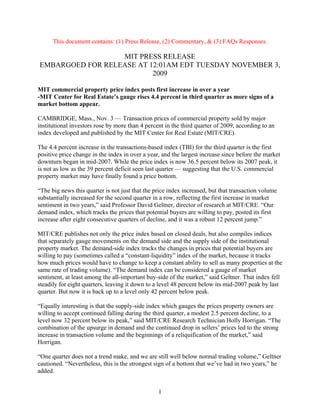
2. “Our latest results relate interestingly to recent results posted by another commercial property
price index whose methodology was developed at the MIT/CRE: the Moody’s/REAL
Commercial Property Price Index – or CPPI – produced by Moody’s Investors Service,” Geltner
noted. “Analysis of that index shows that healthy properties, those that are not in distress, have
only dropped in price about 33 percent from the mid-2007 peak, a similar drop to the supply-side
index we’ve recorded here representing property owners’ willingness to trade, while distressed
properties in the CPPI have fallen 56 percent. The types of properties and owners tracked by the
TBI would generally be less subject to distress than those tracked by the CPPI,” Geltner noted.
The TBI tracks the prices that institutions such as pension funds pay or receive when transacting
commercial properties like shopping centers, apartment complexes and office towers. The MIT
Center’s TBI is based on prices of National Council of Real Estate Investment Fiduciaries
(NCREIF) properties sold each quarter from the property database that underlies the NCREIF
Property Index (NPI), and also makes use of the appraisal information for all of the currently
approximately 6,000 NCREIF properties. Such an index — national, quarterly, transaction-based
and by property type, and tracking demand and supply as well as prices — had not been
previously constructed prior to MIT’s development of it in 2006. NCREIF supported
development of the index as a useful tool for research and decision-making in the industry.
TBI Prices, Demand & Supply : 2001-09Q3
set to 2000Q4 = 100
220
200 TBI
TBI Demand (ConstLiq)
180
TBI Supply
160
140
120
100
80
Jun-09
Jun-07
Jun-08
Jun-05
Jun-06
Jun-03
Jun-04
Jun-01
Jun-02
Dec-07
Mar-08
Sep-08
Dec-08
Mar-09
Sep-09
Dec-04
Mar-05
Sep-05
Dec-05
Mar-06
Sep-06
Dec-06
Mar-07
Sep-07
Sep-03
Dec-03
Mar-04
Sep-04
Dec-00
Mar-01
Sep-01
Dec-01
Mar-02
Sep-02
Dec-02
Mar-03
2

3. Geltner Commentary on 3Q2009 TBI Results…
-David Geltner, November 3, 2009.
In my commentary last quarter I stated: “Now if only the demand side would stop falling, we
would really be back in business.” From that perspective, the third quarter results of the TBI
appear to be “just what the doctor ordered” *…
Demand, Supply & Price Indexes underlying the Liquidity Metric:
260 2001-2009
Price 1984Q1=100, Dem&Sup set to = avg leve
240 Demand
Supply
220 Price
200
180
160
140
120
100
20004
20012
20014
20022
20024
20032
20034
20042
20044
20052
20054
20062
20064
20072
20074
20082
20084
20092
yyyyq
Does the 3Q09 increase of 4.4% in completed transactions prices in the NCREIF database
indicate that 2Q09 was “the bottom” in the current market downturn? To be sure, 4.4% is a solid
uptick, almost a full standard deviation above the TBI price index’s long-term historical mean
quarterly return. But the best reason to think that this may flag a bottom in the market is the
upsurge in the demand-side reservation prices, which posted a whopping +11.8% increase, the
first increase in the eight quarters since the market peak in 2Q2007, and the largest increase in
potential buyers’ prices since the record set in 2Q05 (+17.4%). Indeed, 3Q09 saw the second
largest increase in the demand-side reservation prices since the inception of the index in 1984.
Only the demand side can establish a price bottom in a market.
*
The chart here is similar to the one at the end of the Press Release, except that the indexes are re-leveled with
different starting values. The values in the chart here are set so that the long-run average value level of each of the
three indices (demand, supply, price) is the same across the entire 1984-2009 history of the TBI. This makes sense
under the assumption that over the long run the two sides of the market agree on average with the prices that reflect
the transactions they actually complete (together). The three indices as depicted here are the values on which the
“TBI Liquidity Metric” is calculated (see below).
1

4. Of course, it takes the demand side and the supply side working together to create a functioning
market, and in this regard the property owners also continued to make progress this quarter.
Sellers’ reservation prices posted another decline, after their spectacular fall of last quarter they
eased into a modest decline of another 2.5% in the third quarter (taking the supply side to 31.8%
below its 1Q08 peak). * Combined with the demand jump, this produced a strong upsurge in sales
volume to levels around half of the normal healthy-market volume. Sales out of the NCREIF
index have now increased for two quarters in a row, and are back up to levels that, while still
clearly well below normal, suggest a market that is returning to functionality.
TBI Transaction Volume:
Index Sales Observations as Percentage of NCREIF Properties
7%
6%
5%
4%
3%
2%
1%
0%
2Q 1984
2Q 1985
2Q 1986
2Q 1987
2Q 1988
2Q 1989
2Q 1990
2Q 1991
2Q 1992
2Q 1993
2Q 1994
2Q 1995
2Q 1996
2Q 1997
2Q 1998
2Q 1999
2Q 2000
2Q 2001
2Q 2002
2Q 2003
2Q 2004
2Q 2005
2Q 2006
2Q 2007
2Q 2008
2Q 2009
Our illiquidity measure was more than cut in half in the third quarter, with the TBI market
“Liquidity Metric” jumping from around negative 25% to around negative 11%, meaning that a
further combination of sellers’ reduction in their reservation prices and/or buyers’ increase in
their reservation prices totaling about 11% would bring the market back to full normal liquidity
(characterized by average trading volume). †
*
As noted in the press release, there is an interesting congruence between the TBI price drop and that of the
“healthy” properties in the Moody’s/REAL CPPI (that is, properties not flagged by the Real Capital Analytics
“troubled asset” designation). Through August CPPI healthy properties were down 33% since the October 2007
peak, while through 3Q2009 TBI supply-side reservations are down 31.8% from that index’s 1Q2008 peak,
compared to TBI prices in completed transactions down 36.5% from their 2Q2007 peak. (CPPI properties falling
into distress since October 2007 are down 56%.)
†
Description of the “Liquidity Metric”... This metric (which might also be considered a quantification of a type of
“bid-ask spread”) is constructed in three steps. First, we take the full-history average value levels of the three
indexes (price, demand, supply) based on their official starting values of 100 in 1Q1984. Label these three value
levels as “P”, “D”, and “S”. Then we multiply the demand and supply index value levels at each point in history by a
constant equal to the ratio P/D for the demand index and P/S for the supply index, thus giving all three adjusted
2

5. TBI Liquidity Metric:
30% Buyers' Minus Sellers' Reservation Prices as Fraction of Current
Transaction Price
25% (Assumes Dem, Sup & Price Indexes Equal Avg Level 1984-2009)
20%
(DemandPrice-SuppyPrice)/TransPrice
15%
10%
5%
0%
-5%
-10%
-15%
-20%
-25%
-30%
1984
1985
1986
1987
1988
1989
1990
1991
1992
1993
1994
1995
1996
1997
1998
1999
2000
2001
2002
2003
2004
2005
2006
2007
2008
2009
Nevertheless, a single quarter does not a trend make. There is some noise in the TBI. Second
quarter was so extremely negative, that some part of this quarter’s return may be a sort of
mathematical reaction or “bounce-back”, a correction of negative noise in the second quarter.
Indeed, if market prices assume an essentially flat trajectory for a while, I would expect the TBI
to “bounce along” with a tendency toward alternating slightly positive and slightly negative
quarters. Even so, a flat trajectory would be a turning from the downward plunge of the past two
indexes a full-history average value level of P. Finally we compute the relative liquidity measure each period t as:
(Dt – St)/Pt , based on the index value levels each period as adjusted in step two.
The exact value indicated by this metric is therefore ad hoc, based on the assumption that, over the long
run, the average demand-side reservation price equals the average supply-side reservation price. This assumption is
reasonable, as it acts essentially as a calibrating mechanism, to define the liquidity “neutrality” point (zero bid-ask
spread) to represent the long-run average amount of liquidity (average trading volume turnover) in the market.
However, given the cyclicality in the real estate market this assumption will be most accurate when the total history
since 1Q1984 represents a complete whole multiple of the liquidity cycle (e.g., when the current liquidity level
approximately equals the 1Q1984 NCREIF turnover ratio). As of 3Q2009 we are a bit below that starting liquidity
value (which likely reflected the lack of maturity of the NCREIF property population in 1984 when many funds
were very new, leading to a below long-run average sales ratio even though the real estate market was strong in
1984). This may slightly throw off the liquidity metric (making it too low, probably by less than a point). If we
continue to publish this metric, we will likely “freeze” the historical index value levels from which it is computed
when next the market gets close to its initial 1984 liquidity level or when the full-history average liquidity metric
nears zero (it is presently at -0.6%).
(Note that this liquidity metric is not sensitive to the official starting values of the three indexes in 1Q1984,
which is admittedly arbitrary (at 100) but which cancels out in step two as the index returns each period are
unaffected by merely multiplying the index levels by a constant.)
3

6. years, a sort of “90-degree turn” (not 180 degrees, but better than no turn when you were headed
into a wall).
Of course, as always, much depends on the evolution of the real economy. But barring a double-
dip in the recession, it seems to me that the only force that could drive prices down significantly
below the second quarter’s nadir would be distressed selling, and that is a phenomenon that
should be relatively rare among the NCREIF members’ core properties that characterize the NPI
database tracked by the TBI.
TBI & Corresponding NPI (EWCF) Price Indices: 1984-2009Q3
TBI 1Q84=1, NPI set to = avg level 84-09
2.5
2007
Peak
2006 Pause:
2.0 (condo bust, Int rate
spike)
'87 Stk Mkt
Crash 1998-99
Fin Crisis,
1986 2001-02
REIT Bust
1.5 T ax 1990-91 Recession 2007-9
Reform Recession crash
2005-7 bottom??
R.E.
1.0
Boom
1997
REIT
1992-93
Boom
Kimco T aubman
IPOs
0.5
19841
19851
19861
19871
19881
19891
19901
19911
19921
19931
19941
19951
19961
19971
19981
19991
20001
20011
20021
20031
20041
20051
20061
20071
20081
20091
NPI Appreciation (EWCF) Transactions-Based (Variable Liquidity)
Regarding the properties in the NPI, another metric that the TBI model allows us to report is an
estimate of the difference between the transaction prices tracked by the TBI and the appraisal-
based values reported into the NPI. As of 3Q09 our current estimate would be that the average
NPI reported valuation is down to only about 8% above the corresponding transaction prices in
the third quarter, cut from nearly an 18% spread in the previous quarter. * This derives from a
*
As a percentage of the reported value the difference is now about 7% compared to 15% in the second quarter. We
note that this does not imply that the transaction prices of the properties actually sold during the quarter were below
their then-current appraised (or NCREIF-reported) values for those particular properties. The TBI can only estimate
4

7. combination of the uptick in transaction prices in the TBI combined with continued mark-down
of valuations by NCREIF members (the NPI equal-weighted cash-flow based index capital value
was down 4.2% in 3Q09 *).
A final comment about the trajectory of this down market…
There is evidence in recent academic study of down cycles in the housing market that such down
markets move through three distinct phases related in part to what one might argue are
behavioral phenomena among market participants (sellers and buyers). † The first phase is
characterized by the fall in demand that fundamentally causes the down market but which is
initially combined with loss aversion behavior on the part of sellers (home owners). This results
in a drying up of transaction volume and with such transaction prices as are observable not fully
reflecting the decline in demand. The second phase is characterized by sellers finally reducing
their reservation prices (due to some combination of distressed sales and reality setting in, or
simply the inability to further postpone moving). This drives prices down further even as
transaction volume begins to pick up. Finally, the third stage is the pull up out of the bottom of
the down cycle as (or if ) demand begins to grow again.
It would seem that the history of the TBI over the last two years may conform well to this
stylized model of the down cycle, only with a notable acceleration of the phases as compared to
the housing market. Particularly during 2009 it seems that the private commercial property
market has been able to effect a drastic re-pricing much more quickly not only than the housing
market, but than the commercial market itself has been able to do in past down cycles, such as
the 1970s and 1990s. The TBI price index fell 22% in the first half of 2009, whereas in the
downturns of the 1970s and 1990s commercial property transaction prices fell for more than
three years. If 2Q09 does turn out to be the price bottom, then this downturn would have been
completed in exactly two years in the TBI. Whether this acceleration is due to the role of the
public securities markets in both the equity and debt side of commercial real estate (e.g., REIT
prices began falling in February 2007, well ahead of the private commercial market, and
bottomed at the beginning of March this year), or due to generally better private market
information availability in the 2000s compared to earlier times (characterized, for example, if we
may say so, by transaction metrics such as the TBI and the Moody’s/REAL CPPI), remains to be
determined. But it would indicate in improvement in the informational efficiency of private
commercial real estate.
A note on the sectoral indices:
While the TBI all-property index is up this quarter, all of the sectoral indices are still negative.
This is again a reflection of the different index construction methodology between the aggregate
and sectoral indices which I described in my last quarter’s commentary, due to the smaller
transaction sample sizes in the sectoral indices. Just to repeat, the sectoral indices employ a noise
filter which during the three quarters prior to the last quarter of the calendar year results in an
the difference between transaction price and NPI-reported valuation implicitly for the average (equal-weighted)
property in the NCREIF population.
*
The EWCF version of the NPI adds back the capital expenditures removed from the official NPI appreciation
return, making the capital return of the EWCF version of the NPI comparable to the TBI price index.
†
See for example: Nai Jia Lee, “Panel Data Analyses of Urban Economics and Housing Markets”, PhD
Dissertation, MIT Department of Urban Studies & Planning, September 2009.
5

8. anchoring of these indices to the appraisal-based NPI, causing a lag bias in the sectoral TBI
indices compared to the all-property index, prior to the fourth calendar quarter. With the 4th-
quarter index updates this bias will be corrected (and then the corrected returns frozen into the
indices going forward), as the 4th-quarter anchor for the noise filter will be an annual version of
the TBI transaction-based index.
In the meantime, the all-property TBI should be used as the better gauge of the magnitude of the
overall or average price change. (The all-property index of course has more data to work with,
and it no longer employs the noise filter that pushes returns toward the NPI.) Also, as I have
suggested before, due to the very small sample sizes in the TBI sectoral indexes, readers may
want to consider looking at the Moody’s/REAL CPPI sectoral indexes for a better indication of
sectoral price movements. The third-quarter update of the CPPI sectoral indices will occur on
November 19 by Moody’s. (The CPPI is also a transaction price based index whose
methodology was developed at the MIT/CRE; it is published by Moody’s Investors Service,
though also is available after a lag on the MIT/CRE web site.)
Above commentary reflects the opinion of the author only, not of MIT or the Center for Real
Estate.
6

9. Frequently Asked Questions about the TBI…
Excerpts from email discussions with index users…
Question (Meaning of Price vs Demand Indexes):
“My interpretation is that [the price index] metric represents the average value of all US core real estate
[in the subject sector]. Data is also provided for the "Demand" and "Supply" indices. Is it an
oversimplification to presume these indices suggest the trends in Seller's v. Buyer's asking price?”
Response (DG):
I would say that your interpretation is essentially correct. The (variable-liquidity) price index
reflects the changes in prices in realized transactions, closed deals, and each of those deal prices
of course reflects an agreement between parties on both sides of the market (supply as well as
demand), and therefore the price index reflects the market "equilibrium" price (such as it was at
the end of the time period reported by the index). Equilibrium prices are arguably the most
important single measure because they do represent a sort of "agreement" between the two sides
of the market and they represent actual money changing hands. However, in real estate
transactions prices must be interpreted in the context of trading volume (or "liquidity") that is
highly pro-cyclical in nature, with far less trading in a down market, especially in the early stages
of a sharp downturn. Thus, you can't expect to be able to sell as many properties as quickly or
easily at the equilibrium price in a down-market as at the equilibrium price in an up-market.
(Maybe this matters to you, maybe it doesn't.)
So, to add depth and perspective to the picture, we produce the demand and supply side indexes.
The demand-side ("constant-liquidity") index reflects systematic changes in what economists call
the "reservation price" (or “private valuations”) that potential buyers are willing to pay. This is
not exactly the same thing as a "bid price", which in real estate may only represent an opening
bid where deals are negotiated or put through multiple-round auctions. The same thing is true on
the supply side, only from the perspective of the property owners, the potential sellers. Posted
asking prices (if they even exist) are meant as a signal and perhaps a starting-point for
negotiations. In contrast, the "reservation price" is the price at which the party will stop searching
for an opposite party, stop negotiating, and do the deal. By looking at these two indexes
reflecting reservation price movements on each side of the market you can get a deeper picture of
what is going on underlying the transaction price changes in the market. Keep in mind that the
indexes only reflect the relative changes across time within each index. You cannot relate the
absolute level of any index with that of any other index as of any given time.
As noted, the TBI indexes are "statistical products", which means they can contain some
estimation error, and also they are limited by some simplifying assumptions in their structure.
For example, the underlying econometrics forces the model to assume the same magnitude of
price-elasticity on the demand side and on the supply side. You will note that the difference
between the variable-liquidity price index and the two reservation-price indexes (demand and
supply) is always the same magnitude (just opposite sign) between those two sides of the market.
This reflects the simplifying assumption of equal-elasticity magnitude (always equal across the
two sides, but not constant over time).
1

10. Question (Sufficiency of Number of Observations):
“The MIT website indicated transaction volume was extremely low in Q408, which calls into question
whether there was sufficient data available to support the current index value, particularly at the asset-
class level.”
Response (DG):
Regarding your question about the number of transactions, in effect, the sufficiency of the
sample size, we are getting scarily low. My sense (this is based on my experience and judgment,
not formal statistical science) is that we are still OK at the aggregate level, for the all-property
index. I have less confidence in the individual sectoral indexes. As I suggested on the web site, I
would recommend consulting the Moody's/REAL Commercial Property Price Index for a
transactions-price index that is based on a broader population and hence much larger sample of
transactions, particularly for looking at the sectoral level. The Moody's/REAL CPPI is
comparable to the variable-liquidity (equilibrium) price index version of the TBI, only the
Moody’s index tracks a much larger, broader population of commercial properties based on the
Real Capital Analytics database. (You can download the Moody’s data from either
http://web.mit.edu/cre/research/credl/rca.html
or
http://www.realindices.com/real/index.htm
as well as from Moody's).
Having said that, I must say that the three TBI sectoral indexes that we were able to produce this
time (as noted, we couldn’t do retail due to complete lack of sales), look fairly reasonable to me.
This despite that they have only about a dozen transactions each. We don't have a policy of not
publishing a TBI just because of few data observations, but one certainly does need to keep that
in mind. In general I have been pleased with how reasonably the indexes seem to perform even
with surprisingly few observations. We employ a noise filter that seems to be very effective.
Nevertheless, as I said, I would take the sectoral indexes especially with a grain of salt.
Response Update (DG, 1Q09):
With even fewer observations in the indexes this quarter, I need to reiterate the above points.
However, I should also say that I continue to be impressed (even more so) with the reasonable
and relatively stable nature of the index returns in the face of less data than I expected we would
ever have when we initially developed the TBI methodology. This has caused me to re-think how
the indexes are working, and to see a strength in their structure that I did not originally consider.
As noted in my commentary this period, I believe the TBIs’ stability in the face of scarce data
results from two main factors: (i) the quality of the main hedonic explanatory variable in our
price model, the regularly-updated manager-reported valuations of the properties; and (ii) the
pooled nature of the estimation database, which enables the thousands of transaction prices in the
historic data to all be used in the model estimation process each period. This stability
(smoothness in the indexes), as well as the prima facie reasonableness and believability of the
index results, speaks to the accuracy of the indexes. Their ability to register turning points in the
market prior to the appraisal-based NPI speaks to their ability to discover transaction-price-based
information about market movements ahead of the NPI. Nevertheless, the TBI’s price models’
standard errors are quite large relative to the size of typical quarterly returns or quarterly
volatility. There is certainly some noise in the indexes, though apparently much less than would
be implied by a simplistic application of the time dummy-variable coefficient standard error
magnitudes in the price regressions (which are in the range of 4% to 8% each period).
2

11. Question (Role of Appraisals in the TBI):
“While the information provided on the MIT website seems to suggest that the index is impacted only by
actual transactions, your research paper on the topic also discusses the use of appraised values as
reported by the NPI in the TBI. I would appreciate knowing exactly how the TBI incorporates appraised
values, if at all.”
Response (DG):
Regarding your question about how the appraised values are used in the transaction price index,
the appraised values are just a right-hand-side variable in the regression to control for qualitative
differences cross-sectionally across the properties (such as size, quality of location, age, etc). The
dependent variable in the regression is only the actual transaction price (per SF), hence, the index
is truly a transaction price based index, not appraisal based. (Maybe I should clarify, the index
measures "longitudinal" movements, changes through time, and it does so based purely on
changes in transaction prices, not appraised values.)
Response Update (DG 1Q09):
As discussed in the 1Q09 update of my response to the previous question, I would now say that
the above answer does not give full credit to the role of the “appraisals” in the TBI. (I put
“appraisals” in quotes because, more accurately, the values we use as the main hedonic variable
in the TBI models are the manager-reported “official” valuations of the properties that are
reported into the NPI each quarter. These manager-reported valuations have traditionally been
largely based on independent fee appraisals or in-house appraisals of the properties.) The
NCREIF appraisals are updated regularly and frequently, even if not always every quarter for
every property. The frequency, and “seriousness”, of the updating process seems to have gotten
greater in recent years. And during the 2007-09 market collapse the updating process has become
even more aggressive (especially starting in 4Q08). Thus, the main hedonic variable in the TBI
price model is not just cross-sectional in nature, but has an important longitudinal component as
well.
Response Update (DG 2Q09):
As noted in my commentary for 2Q09, the NPI “appraisals” (more correctly, the property
owners’ reported values) serve a temporary role for the TBI sectoral indexes’ preliminary returns
which are issued prior to the fourth calendar quarter each year. During calendar quarters one
through three the noise filter used in the sectoral indexes “anchors” to the corresponding NPI
capital returns (with the NPI defined on an equally-weighted cash flow basis comparable to the
TBI). With the 4th quarter update each year these indexes prior quarterly returns during the latest
calendar year are “re-anchored” to a calendar-year annual frequency transaction-based index (an
annual frequency version of the TBI’s hedonic price model without any noise filter). It is these
re-anchored and fully updated quarterly returns which then get “frozen” going forward after the
end of the calendar year. Thus, the NPI appraisals can have some influence on the sectoral level
TBI indexes during the three preliminary quarters of the current year prior to the 4th-quarter
updating and “freezing” (but not on the all-property index). This can cause some lag bias in the
preliminary sectoral indexes, the more so the more lagged the NPI is and the scarcer are the
transaction observations.
3

12. Question (Backward Adjustments, 4Q08):
“We have noticed significiant historical revisions in the price series. Were the revisions larger than
normal, and is there a story behind them?”
Response (DG):
Regarding backward-adjustments, they may have been a bit larger than normal this time,
probably due to the sharp turn in the market during calendar year 2008. As noted on the web site,
we consider the "TBI" to be "preliminary" through the first three quarters of each year, then
"finalized" (though there can still be further backward adjustments) with the 4th-quarter report.
This is due to technical reasons which I will briefly explain here...
We use a ridge regression noise filter in the index. This is a Bayesian technique that works by
biasing the return estimates towards an "anchor". The anchor is the transactions-based index
estimated at the annual frequency at the end of every calendar year. By estimating at the annual
frequency we have much more data in each period and hence less noise. (We also control for
temporal aggregation at the annual frequency, so we avoid lag bias.) But we can only update that
transactions price based anchor at the end of the calendar year. During the interim (other three
quarterly indexes) we use the appraisal-based NCREIF Index as the anchor. The appraisal-based
index is lagged, and that made an especially large difference during 2008 because of the sharp
turn in the market. This is probably why the backward-adjustments were larger in 4Q08 than
they usually are. The most recent index should be considered to be the most up-to-date and
accurate for the historical returns.
Response Update (DG 1Q09):
This relates to the technical changes we are instituting in the TBI starting in 1Q09. From now on,
there should be no backward adjustments to returns prior to the current calendar year, as we are
“freezing” the indexes at the end of each calendar year as a matter of policy. This is being done
to improve the practical usefulness of the indexes, and considering that backward adjustments
have always been minimal and generally of no economic significance (particularly after the end
of the calendar year). Also, we have adjusted the noise filter, eliminating it altogether in the
aggregate all-property index. Analysis indicates that the noise filter is no longer necessary at the
aggregate level, and eliminating it will increase the independence of the TBI from the NPI during
the preliminary reports in the interim quarters.
Question (Index Base Period & Levels Comparisons):
“I was hoping you could tell me the base year for the transactions-based index. I think it might be 1983,
but I was hoping you might be able to confirm for me.”
Response (DG):
The base period is 1Q1984 (first return period 2Q1984) for the national aggregate index, and
1Q1994 for the sectoral indexes.
The base periods’ index values for the TBI are not necessarily equal to 100. As you know, the
base period value of an index (any index) is arbitrary. The meaningful information in the index is
the periodic returns (relative changes starting from the base period). What our program does is to
set the base period index value level to whatever level will give the TBI index levels an average
value (across the entire history) equal to the average value level of the corresponding NCREIF
Index in which the latter’s base period value is set (arbitrarily) to 100. (We could have done it
the other way round – it’s just arbitrary we picked the NPI to set to 100.) This is done purely for
4

13. visual display in the graphs. In reality there is no rigorous comparison between the index value
levels between the NPI and TBI indexes. You can’t say that transaction prices were 5% above
appraised values just because the TBI (capital index) happens to be, say 210 in a period when the
NPI is 200. (However, if the next period the TBI moves to 189 and the NPI moves to 190 then
you CAN say that period the transaction prices moved down 10% while the appraised values
moved down 5%.) The reason we set the starting values as we do for visual purposes in the
graphs is that, as an approximation, it does make sense to assume that appraised values and
transaction prices will tend to have equal average values over the long run. While lagging and
smoothing in the appraisal-based index will cause its returns to differ from the transaction-based
returns over short-to-medium spans of time, over longer historical spans of time involving full
“cycles” in the real estate market the differences between appraisals and transactions tend to
cancel out: Appraisers tend to follow the market, just with some lag and perhaps smoothing off
the peaks and valleys a bit.
Response Update (DG 1Q09):
We have now (as of 1Q2009) decided to indeed flip it around, and set the TBI indexes to all have
starting values of 100 at their inception dates, and make the NPI’s starting value (in our charts)
float to the value that gives it the same overall average level as the corresponding TBI. It seems
to make more sense, and to reduce confusion, to have the TBIs start at 100, since those are the
indexes we are producing and publishing.
Response Update (DG 2Q09):
See the subsequent question and response below entitled: “How can demand index exceed
supply index?”.
Question (Aggregate index not composite, & missing retail 4Q08):
“I am trying to retrieve data on your Transactions-Based Index and it appears as though the fourth-quarter
data for the retail segment is missing. It is present for the office, industrial, apartment and composite
index, however. If the composite was calculated I would assume the retail data is available. If you can
provide any feedback I would really appreciate it. Thank you very much.”
Response (DG):
We could not publish a retail index for 4Q08 because there were no sales of retail properties out
of the NCREIF database that quarter. The aggregate index is not a composite built up from the
sectoral indexes, but rather is an independently-estimated regression based on the entire data
sample of sold properties as if they were all members of a single population.
Response Update (DG 1Q09):
We have now updated and “backfilled” the retail index, by “straightlining” the index from 3Q08
through 1Q09 (in effect, assuming equal returns in 4Q08 and 1Q09). This is done on the basis of
only a single retail sales observation in 1Q09. Nevertheless, the result seems broadly reasonable
(retail down 7.3% over the two quarters, which we have apportioned as -3.7% in each quarter,
geometric: (1 – 0.073) = (1 – 0.037)*(1 – 0.037), with round-off). This is consistent with our
previously-stated policy of reporting an index result whenever we can calculate one. (In the
future, we may nuance this policy, reserving the right to not report a result if there is very scarce
data and the result seems spurious or unreasonable. However, this is not the case in the present
instance.)
5

14. Response Update (DG 2Q09):
The straightlined, backfilled retail index was frozen at the end of 4Q2008, but the index
remained subject to updating and backward revision during the subsequent three quarters of CY
2009, with those revisions applying to all CY2009 quarters subsequent to the 4Q08 freezing.
Thus, only the first of the two original equal backfilled quarters (4Q08 & 1Q09) remains at its
original backfilled value of -3.7%.
Question (NPI capital index tracks below TBI long-term):
“I was trying to compare the MIT TBI Index with the NCREIF Capital appreciation index - I understand that
there is a slight lag between the two indices - however, in terms of magnitude, I expected them to match
up (for e.g., similar to your chart shown below, where you show inflation adjusted price series). I wanted
to ask if you expect so much difference between capital appreciation being implied by the two series?”
Response (DG):
Keep in mind that the NPI official index differs from the TBI in two respects that affect direct
comparisons of the capital returns.
First, the official NPI is value-weighted, larger property’s returns count more heavily in
computing the index return. The TBI is equal-weighted, all properties count the same. We use
the equal-weighted version in the TBI because we view the TBI as essentially a statistical
estimation, based on a sample of properties (the ones that sold) inferring from that sample the
change in value in the market represented by the entire NCREIF population of properties. We
view each sold property as an equally-valid representative of that population. Hence, it makes
sense for us to use the equal-weighted version of the NPI for comparison purposes. Also, the
equal-weighted NPI tends to have less volatility (in effect it is more diversified, less dominated
by a few large properties). You can download the equal-weighted version of the NPI from the
NCREIF website, via the custom query screen. However, the difference between equal-wtd vs
value-wtd does not produce a systematic trend difference that would cause the index levels to
diverge over time, which is what is bothering you, so this EW vs VW difference is not the
answer to your question.
Second, the official NPI “capital return” (or “appreciation return”) removes capital expenditures
from the change in asset value that forms the numerator of the capital return computation. For
example, suppose a property was worth $100M at the beginning of the quarter and $105M at the
end of the quarter but had $1M of capital expenditures spent on it during the quarter, then the
NPI would compute the capital (or appreciation) return as 4%, not 5%. Suppose the property also
generated $7M of NOI during the quarter. The official NPI would record the “income return” as
7%, even though only $6M of cash would have been available to the property investors after the
CapEx. The NPI total return would be 4% appreciation + 7% income = 11%. This differs from
the way stock market index returns are computed in terms of the breakout between capital and
income. The income component is based only on paid-out dividends (not booked earnings), and
the capital return is based on the stock price change no matter how much of that value change
may reflect retained earnings plowed back into the company. If the properties described above
were a stock the capital return would be 5% and the income return would be 6% (for the same
total return of 11%). We do the TBI like a stock index. We don’t remove CapEx from the TBI
price index, as we mean that index to track commercial property price changes (for same
properties), including the effect of (routine) capital expenditures on the properties. (The NPI and
TBI do not include development or redevelopment or major rehab properties.) You can
6

15. download from the NCREIF website (via the custom query screen) a redefined version of the
NPI capital and income return components defined as we do in the TBI, based on cash flows
rather than book earnings. We use this redefined version of the NPI components in order to make
the comparisons that we show on our charts. We call this the “EWCF” version of the NPI (equal-
wtd, cash flow-based), and it is what we use in our charts. If you just compare the TBI price
index with an NPI based on the official NCREIF capital (appreciation) returns, the NPI will trend
below the TBI (even apart from smoothing or lagging effects) due to the removal of (on average
about) 2%/year of capital expenditures from the official NPI capital index.
Question (How can demand index exceed supply index):
“The data is extremely interesting and useful, however, I don’t understand how Demand (or the bid) is
ever greater than the Supply (or the ask). Meaning if the sellers were willing to sell the assets at a lower
price than the buyers were willing to pay then the transaction would just execute and we would see the
bid and ask be the same. Your data shows years when the Demand is greater than the Supply and I was
hoping for an explanation as to what that means.”
Response (DG):
The indexes (all of them, not just demand and supply) actually only quantify percentage changes
over time within the given index. That is, the price index only actually tells us how much
realized (closed deals) transaction prices have changed; the demand index only tells us how
much the potential buyers’ (average) reservation prices have changed; and the supply index only
tells us how much the property owners’ reservation prices have changed, between any two points
in time (since the indexes began). They do not rigorously tell us the relative price levels across
the indexes as of any point in time. In principle in a rigorous sense you cannot compare index
levels across indexes, only within an index across time. The starting value of each index is
arbitrary (set at 100). This does not imply that all the indexes (price, demand, supply, total
return) were actually at the same level at the inception date of the indexes (1Q1984 for the all-
property indexes). Each index simply equals its starting value (call it “S(0)”, an arbitrary
number) grown forward from the inception date at the actual accumulated (compounded) returns
registered by the index each period:
S(t) = (1+r(t))*(1+r(t-1))*(1+r(t-2))*…*S(0), (1)
where “r(t)” is the index return in period “t” (since the inception date). It is only the returns (the
“r(t)” values for each “t” since inception) that are the actual “data” provided by the indexes, in a
rigorous sense.
Having said that, one can nevertheless make some plausible and interesting comparisons (I think)
across index levels, less formally, by making some reasonable assumptions (in effect, about
relative differences in starting values). For example, in the charts that we produce for the TBI we
put the TBI price index and the NCREIF Property Index side-by-side on the same chart for visual
comparison purposes. To do this we re-set the starting value of the NPI (effectively multiplying
each value level of that index by a constant) so as to equalize between the two indexes the
average index value levels across the entire index history. This makes some sense as an
approximation of the relation between the two indexes’ value levels, because on average over the
long run the appraised values represented by the NPI are probably unbiased, that is, on average
the appraisers are right over the long run (at least approximately, and as a practically useful
assumption). Lagging and smoothing does not cause the long-run average NPI-reported valuation
7

16. to be biased; it just causes the current valuations to be biased on average (in one direction or the
other at a given time depending on which way the market has been moving).
In a similar spirit, in our chart of the demand and supply indexes we (arbitrarily) re-set the
starting value of the supply index to give it the same long-run average value level as that of the
demand index. Again, this does not affect the periodic returns, the actual data rigorously in the
indexes, as the index level is adjusted only by multiplying each level by a constant which cancels
out in the return: r(t) = S(t)/S(t-1)-1. (See what happens in this ratio to S(0) when you plug
formula (1), above, into this return formula.) In effect, this index level adjustment calibrates the
demand and supply indexes so that they will be equal (or approximately equal) in levels during
times when the institutional property market is at a “normal” or “average” level of liquidity
(trading volume is at a typical level, not exceptionally “hot” nor exceptionally “cold”). Formally
speaking, this is an ad hoc calibration. But hopefully you can see the logic and intuition in it.
(However, please note the second paragraph in the footnote on page 3 of my “commentary” to
our 2Q09 release of the TBI, downloadable from the Center’s website this quarter.)
So to come around finally to your original question: how can the demand index ever be above
the supply index?... Based on the calibration I just described, this would happen when the
demand is relatively strong, that is, when potential buyers’ are moving their reservation prices
relatively higher compared to their long-run average, and relative to the reservation prices of the
property owners. As you can see from the chart of the “Liquidity” measure on page 2 of the
2Q09 commentary (the sign of that measure is based on the difference between the demand
index level minus the supply index level), the demand index exceeds the supply index calibrated
in this way during the major “boom” periods of price appreciation during the late 1990s and the
2003-07 period. (Of course, one can get a different visual perspective by recalibrating the
indexes, for example, the chart at the end of the press release sets all indexes to have equal
values of 100 at the end of the year 2000, to emphasize changes only since then.)
Naturally, there are many (and heterogeneous) potential buyers, and similarly many
heterogeneous potential sellers. Whenever a transaction is consummated it means that one of
those buyers had a reservation price that was at least as high as the reservation price of one of
those sellers. (The transaction price occurs somewhere between the buyer’s and seller’s
reservation prices, the outcome of their negotiation process.) Greater transaction volume (greater
turnover in the market) indicates that there are proportionately more such overlaps in the
population (relatively more buyers whose RPs exceed those of sellers). Think of there being a
frequency distribution of all of the potential buyers as a function of their RPs; and another
frequency distribution of all of the potential sellers as a function of their RPs. These two
frequency distributions overlap on some range of prices, and that price range is where the trading
happens. The TBI demand and supply indexes measure the movements (across time) in the
average values of each of those frequency distributions of RPs (assuming each side of the market
has the same range or variance in their distribution).
If you want a more in-depth explanation of how the demand and supply indexes work (including
a graphic that illustrates the overlapping buyer & seller distributions I was referring to in the
previous paragraph), you can download the technical documentation of the TBI from the “Fisher,
Geltner & Pollakowski” link on the Center’s TBI web-page (it’s in the section titled: “TBI
8

17. Details & Usage”). The graphic is in Exhibit 1 on page 39 of that paper, and it is discussed on
pp. 7-12 of the manuscript.
9