X ray diffraction basics

Diffraction Basics

Introduction
The utilization of X-ray diffraction for crystallographic analysis relies on a few basic
principals:
1. When an incident beam of x-rays interacts with a target material, one of the primary
effects observed is scattering (spherical radiation of the incident x-rays without
change in wavelength) of those x-rays from atomic scattering centers within the target
material.
2. In materials with some type of regular (i.e., crystalline) structure, x-rays scattered in
certain directions will be in-phase (i.e., amplified), while most will be out of phase.
This is the process of diffraction.
3. Measurement of the geometry of the diffracted x-rays can be used to discern the
crystal structure and unit cell dimensions of the target material.
4. The intensities of the amplified x-rays can be used to work out the arrangement of
atoms in the unit cell.
For the x-rays to yield useful information about the material structure, the wavelength of the
incident x-rays should be of that same order of magnitude as the interatomic spacing in the
crystal structure.
In this section we will discuss this process of diffraction and how we make use of the
amplification and attenuation to elucidate the structure of the material(s) in the target. The
goal of this section is to give the student sufficient background in the mathematics and
crystallography underlying the practice of x-ray diffraction so that the analytical results will
rise above the level of a “black box” technique.
The first part of the material (including the illustrations) in this section is abstracted from
Chapter 3 of Nuffield (1966). The remainder of the material (from Bragg’s Law on and the
reciprocal lattice) is from Jenkins and Snyder (1996) and Bloss (1994). I thank Dr. Cornelis
Klein for his suggestions and assistance with this material.

The Geometry of Diffraction
As discussed previously, there are many types
of secondary effects that occur when x-rays
interact with matter. Fortunately the dominant
effect, and the only one with which we are
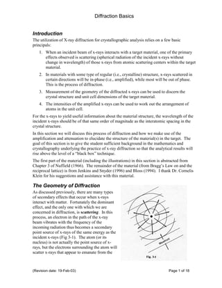
concerned in diffraction, is scattering. In this
process, an electron in the path of the x-ray
beam vibrates with the frequency of the
incoming radiation thus becomes a secondary
point source of x-rays of the same energy as the
incident x-rays (Fig 3-1). The atom (or its
nucleus) is not actually the point source of x-
rays, but the electrons surrounding the atom will
scatter x-rays that appear to emanate from the

(Revision date: 19-Feb-03) Page 1 of 18

Diffraction Basics

center of the atom.
A crystal is a complex but orderly arrangement of atoms, and all atoms in the path of an x-
ray beam scatter x-rays simultaneously. In general, the scattered x-rays interfere, essentially
canceling each other out. In certain specific directions, where the scattered x-rays are “in-
phase” the x-rays scatter cooperatively to form a new wave. This process of constructive
interference is diffraction.
The directions of possible diffractions depend only on the size and shape of the unit cell.
Certain classes of diffraction are systematically extinguished by lattice centering and by
certain space-group symmetry elements. The intensities of the diffracted waves depend on
the kind and arrangement of atoms in the crystal structure. It is the study of the geometry of
diffraction from a crystal that we use to discern the unit cell dimensions; the missing
diffractions give the symmetry of the crystal. The intensities are used to work out the
arrangement of atoms.
The Laue treatment of the geometry of diffraction, developed by Max von Laue in 1912, is
presented in the following sections because of its geometric clarity and the rigor with which
the concepts are treated. As will be discussed, Laue diffraction occurs with polychromatic
(i.e., “white”) rather than monochromatic radiation that we use with powder diffractometry.
Later we will present Bragg’s treatment of diffraction that allow diffraction of
monochromatic x-rays to be treated as reflection. Bragg’s treatment greatly simplifies the
mathematics involved in diffraction calculations, and, when combined with the somewhat
difficult but very useful concept of the reciprocal lattice, simplifies the experimental
measurement of a diffraction pattern, thus making diffraction a useful routine tool for
crystallographic studies.

Diffraction by a Row of Identical, Equally Spaced Atoms
Consider the
hypothetical case of a
one-dimensional row of
equally spaced atoms.
Each atom in the path of
an x-ray beam can be
considered to be the
center of radiating,
spherical wave shells of
x-rays (Fig 3-2).
In general the scattered
waves interfere, cancel
out and no diffraction
occurs. However, when
the scattered waves
happen to be in phase,
they form wave fronts as
shown in Figure 3-2. Since wavelengths of λ, 2λ and 3λ will all add to produce a different
wavefront, we call these first-, second- and third-order wavefronts. By convention,


Diffraction Basics

wavefronts to the right of the diffracted beam is are positive, those to the left are negative
(i.e., minus first-order, etc.).

Figure 3-3. Condition for diffraction from a row
Figure 3-3 illustrates the conditions for diffraction from a row of atoms. Two x-rays strike
the row of periodicity p, at an angle of incidence µ , to form zero-, first- and second-order
diffractions. The angle of diffraction, ν , is measured from the left (positive) end of the row.
The diffracted rays are only in phase if:
p (cosν − cos µ ) = ± hλ
where h is the order of the diffraction, in this case 0 or 1. The condition for diffraction is met
not only in the directions AD, AE and AF shown in the diagrams, but in all directions that
make angles of ν , ν ′ and ν ′′ . These outline three concentric cones as shown in figure 3-3d.
The cones define the locus of in-phase scattering (diffraction).


Diffraction Basics

The expression above is the Laue equation for diffraction by a row. Note that for zero-order
diffractions, h = 0, and thatν is equal to µ . The significance of this is that the incident beam
is always a line in the zero-order cone.
When the angle of incidence, µ , is 90°, the Laue equation reduces to:
p cosν = ± hλ

Under this condition the
angleν for zero order
diffractions is also 90° and
the zero-order cone has the
shape of a disk. Higher-
order cones occur in pairs,
symmetrically placed about
the zero-order disk (Fig. 3-4)

Diffraction by a Plane Lattice-Array of Atoms
A plane lattice-array of atoms (Fig. 3-5) may be defined by two translation periods, a and b,
in the rows OA and OB and the angle γ. Basically this extends the concept of diffraction by a
row to include simultaneous diffraction by two non-parallel rows of atoms.
The diffraction directions for the row OA comprise a set of concentric cones coaxial with OA
(Fig 3-5b), and have half-apical angles defined by the Laue equation for a row. The
directions for the row OB comprise another set of cones (Fig 3-5c) with a different
orientation.
When both diffractions are combined, only at the intersection of the diffraction cones will
diffraction occur (since the other diffractions will interfere and thus cancel). Those lines of
intersection are shown as OX and OY (Fig 3-5d). The Laue equations for diffraction by the
plane may be expresses in terms of the Laue equations for the rows OA and OB:
a(cosν 1 − cos µ1 ) = ± hλ
b(cosν 2 − cos µ 2 ) = ± kλ
where a and b are periods of the rows
µ1 and µ 2 are the angles at which the beam meets the rows
ν 1 and ν 2 are the diffractions angles referred to the respective rows.


Diffraction Basics

Diffraction occurs when the two equations are simultaneously satisfied, i.e., when the angles
ν 1 and ν 2 define the same direction. As illustrated in Fig 3-5d, when the beam meets the
plane at such an angle that the hth-order cone about OA intersects the kth-order cone about
OB along OX and OY. The angle between OA and OX (and OY) is ν 1 and that between OB
and OX is ν 2 .

Diffraction by a Three-Dimensional Lattice-Array of Atoms

The diffraction
directions for a three-
dimensional array may
be described by three
sets of diffraction
cones coaxial with
three non-coplanar
reference rows (Fig 3-
6). In general, each
cone will form two
diffraction lines by
intersection with each
of the other two


Diffraction Basics

resulting in 6 diffraction lines shown as OU and OV (a-c) , OY and OZ (a-b), OW and OX (b-
c). For the material to diffract (i.e., interfere constructively) the three diffractions OV, OW,
and OY would need to be coincident, a condition satisfied by the following Laue equations
only when the diffraction angles, ν 1 , ν 2 and ν 3 define a common direction:
a(cosν 1 − cos µ1 ) = ± hλ
b(cosν 2 − cos µ 2 ) = ± kλ
c(cosν 3 − cos µ 3 ) = ±lλ
The a, b and c directions are fixed (and define the unit cell), thus the ν values depend on µ
(the angle at which the beam meets the reference rows) and λ, (the wavelength of the
incident radiation). The possibility of satisfying the three equations simultaneously can be
increased by varying either µ or λ during analysis. In Laue diffraction, the crystal position
in the beam is fixed, and λ is varied by using continuous (or “white”) radiation while keeping
the orientation of the crystal fixed. Monochromatic radiation is used in most modern
diffraction equipment, so for single crystal analysis the crystal must be progressively moved
in the X-ray beam to vary µ sufficiently so that diffractions may be obtained and recorded.
Below is a sample Laue diffraction pattern (Fig 7.39 from Klein, 2002).

The table below summarizes the different diffraction methods and the radiation used. Most
of this course will be concerned with powder methods.


Diffraction Basics

Radiation Method
White Laue: stationary single crystal
Monochromatic Powder: specimen is polycrystalline, and therefore
all orientations are simultaneously presented to the
beam
Rotation, Weissenberg: oscillation,
De Jong-Bouman: single crystal rotates or oscillates
about chosen axis in path of beam
Precession: chosen axis of single crystal precesses
about beam direction

Diffraction as Reflection: The Bragg Law
In 1912, shortly after von Laue’s experiments were published, Sir W.L. Bragg discovered
that diffraction could be pictured as a reflection of the incident beam from lattice planes. He
developed an equation for diffraction, equivalent to the simultaneous solution of the three
Laue equations by monochromatic radiation, which allows diffraction to be treated
mathematically as reflection from the diffracting planes.
Nuffield’s (1966) explanation of the
Bragg condition is particularly clear. In
Figure 3-7 at left, an x-ray beam
encounters a three dimensional lattice-
array of atoms shown as rows OA, OB
and OC. In this case we assume that the
third-order cone about OA, the second-
order cone about OB and the first-order
cone about OC intersect in a common line
to satisfy the Laue condition for
diffraction.1
The x-rays scattered by adjacent atoms on
OA have a path difference of three
wavelengths, those around OB have a
path difference of two wavelengths and
those around OC, one wavelength
difference. These three points of coherent
scatter define a plane with intercepts 2a, 3b, 6c. The Miller index of this plane (the
reciprocal of the intercepts) is (321). Because A’’, B’’ and C’’ are six wavelengths out of

1
Keep in mind that diffraction is not really reflection, but coherent scattering from lattice points, such that each
point may be thought of as an independent source of x-rays. Diffraction occurs when the scattered x-rays are in
phase.


Diffraction Basics

phase with those scattered at the origin, they scatter waves that differ by zero wavelengths
from one another.
To maintain the same path
length (and remain in phase)
the rays must pass through
the plane (Fig 3-8a) or be
deviated at an angle equal to
the angle of incidence, θ (Fig
3-8b). Though it is not really
reflecting the X-rays, the
effective geometry is that of
reflection. Since the lattice is three-dimensional and any lattice point will act as the origin,
(321) defines an infinite number of parallel planes that diffract simultaneously. The
relationship may be stated as follows: A diffraction direction defined by the intersection of
the hth order cone about the a axis, the kth order cone about the b axis and the lth order
cone about the c axis is geometrically equivalent to a reflection of the incident beam from
the (hkl) plane referred to these axes. This geometric relation provides the basis for Bragg
diffraction. Referring to Figure 3-7, diffraction from each parallel plane shown will be
exactly one wavelength out of phase at the proper value of θ.
Figure 3-9 shows a beam of
parallel x-rays penetrating a stack
of planes of spacing d, at a
glancing angle of incidence, θ.
Each plane is pictured as
reflecting a portion of the
incident beam. The “reflected”
rays combine to form a diffracted
beam if they differ in phase by a
whole number of wavelength,
that is, if the path difference AB-
AD = nλ where n is an integer.
Therefore
d
AB = and
sin θ
d
AD = AB cos 2θ = (cos 2θ )
sin θ
d d
Therefore: nλ = − (cos 2θ )
sin θ sin θ
d d
= (1 − cos 2θ ) = (2 sin 2 θ )
sin θ sin θ
nλ = 2d sin θ
The last equation is the Bragg condition for diffraction.


Diffraction Basics

The value of n gives the “order” of the diffraction. Note that the value of the diffraction
angle, θ, will increase as the order of diffraction increases up to the limit where nλ = 2d. The
diagram below (from Bloss, 1994) illustrates this graphically. A indicates light reflection
from a polished (111) face of an NaCl crystal. B indicates diffraction by Cu Kα x-rays at
successive orders of diffraction, with the first-order diffraction at θ = 13.7° (2θ = 25.4°). C
shows the wavelength difference producing the different orders of diffraction. These
reflections are commonly referred to as multiples of the Miller index for the planes without
the parentheses, i.e., 111, 222, 333, 444, but are represent the same value of d.

It can be easily shown that Bragg diffraction occurs in any set of planes in a crystal structure.
Because of geometrical considerations related to multiple out-of phase diffractions (a.k.a.
extinction) in some types of point groups and space groups, not all lattice planes will produce
measurable diffractions. As will be discussed later, these missing diffractions provide
valuable information about the crystal structure.

The Reciprocal Lattice
The most useful method for describing diffraction phenomena has the intimidating name
“reciprocal lattice.” It was developed by P.P. Ewald, and is also called “reciprocal space.” It
makes use of the reciprocal of dhkl to fabricate a geometrical construction which then serves
as a very effective way to understand diffraction effects. Most of the discussion in this
section is abstracted from Jenkins and Snyder (1996).
When setting up an arrangement of x-ray source, specimen and detector, it is useful to be
able to predict the motions that will have to be applied the various motions that will have to
be applied to see particular diffraction effects. Consider the diffraction from the (200) planes
of a (cubic) LiF crystal that has an identifiable (100) cleavage face. To use the Bragg
equation to determine the orientation required for diffraction, one must determine the value
of d200. Using a reference source (like the ICDD database or other tables of x-ray data) for
LiF, a = 4.0270 Å, thus d200 will be ½ of a or 2.0135 Å. From Bragg’s law, the diffraction
angle for Cu Kα1 (λ = 1.54060) will be 44.986° 2θ. Thus the (100) face should be placed to
make an angle of 11.03° with the incident x-ray beam and detector. If we had no more


Diffraction Basics

complicated orientation problems, then we would have no need for the reciprocal space
concept. Try doing this for the (246) planes and the complications become immediately
evident.
The orientation
problem is related to
the fact that the
diffracting Bragg
planes are inherently
three dimensional.
We can remove a
dimension from the
problem by
representing each
plane as a vector –
dhkl is defined as the
perpendicular
distance from the
origin of a unit cell to the first plane In the family hkl as illustrated in Figure 3.2. While this
removes a dimensional element, it is evident that the sheaf of vectors representing all the
lattice planes (see Fig. 3.3 on the following page) will be extremely dense near the center and
not ultimately very useful.
Ewald proposed that instead of plotting the dhkl vectors, that the reciprocal of these vectors
should be plotted. The reciprocal vector is defined as:

1
d* ≡
hkl
d hkl
Figure 3.3 can now be reconstructed plotting the reciprocal vectors instead of the dhkl vectors.
Figure 3.4 shows this construction. The units are in reciprocal angstroms and the space is
therefore a reciprocal space. Note that the points in this space repeat at perfectly periodic
intervals defining a space lattice called a reciprocal lattice. The repeating translation vectors
in this lattice are called a*, b* and c*. The interaxial (or reciprocal) angles are α*, β* and γ*
where the reciprocal of an angle is defined as its complement, or 180° minus the real-space
angle. For orthogonal systems the angular relations are quite simple. For non-orthogonal
systems (monoclinic and triclinic), they are more complex.


Diffraction Basics

The reciprocal lattice
makes the
visualization of
Bragg planes very
easy. Figure 3.4
shows only the (hk0)
plane of the
reciprocal lattice.
To establish the
index of any point in
the reciprocal lattice,
count the number of
repeat units in the
a*, b*, and c*
directions. Fig. 3.4
shows only the hk0
plane, but the lattice
is fully three
dimensional. When
connected, the
innermost points in
the lattice will define
a three-dimensional
shape that is directly related to the shape of the of the real-space unit cell. Thus the


Diffraction Basics

symmetry of the real space lattice propagates into the reciprocal lattice. Any vector in the
lattice represents a set of Bragg planes and can be resolved into its components:

d hkl = ha * + kb * + lc *
*

In orthogonal crystal systems, the relationship between d and d* is a simple reciprocal. In
non-orthogonal systems (triclinic, monoclinic, hexagonal), the vector character of the
reciprocals complicates the angular calculations. The figure at left shows the relations for the
ac plane of a monoclinic unit cell. d001
meets the (100) plane at 90°. Because the
angle β between the a and c directions is
not 90°, the a unit cell direction and the
d100 are not equal in magnitude or
direction, but are related by the sin of the
angle between them. This means that the
reciprocal lattice parameters d*100 and a*
will also involve the sin of the interaxial angle.
Table 3.1 (at right)
lists the direct and
reciprocal space
relationships in the
different crystal
systems. The
parameter V shown
for the Triclinic
system is a
complicated
trigonometric
calculation required
for the this system
because of the
absence of 90°
angles. It is derived by Jenkins and Snyder (1994, p. 53) and listed below:
1
V* = = a * b * c * (1 − cos 2 α * − cos 2 β * − cos 2 γ * +2 cos α * cos β * cos γ *)1 / 2
V

The Ewald Sphere of Reflection
Figure 3.6 (following page) shows a cross section through an imaginary sphere with a radius
of 1/λ with a crystal at its center. The reciprocal lattice associated with the crystal’s lattice is
viewed as tangent to the sphere at the point where an x-ray beam entering from the left and
passing through the crystal would exit the sphere on the right. The Ewald sphere contains all
that is needed to visualize diffraction geometrically.


Diffraction Basics

Rotation of the
crystal (and its
associated real-
space lattice) will
will also rotate the
reciprocal lattice
because the
reciprocal lattice is
defined in terms of
the real-space
lattice. Figure 3.7
shows this
arrangement at a
specific time when
the (230) point is
broght into contact
with the sphere.
Here, by definition:
1
CO = and
λ
d *( 230 )
OA = hence
2
OA d *( 230) / 2
sin θ = =
CO 1/ λ
or
2 sin θ
λ=
d *( 230 )
from the definition
of the reciprocal
vector:
1
d ( 230 ) ≡
d *( 230)
therefore:
λ = 2d ( 230 ) sin θ
which is the Bragg
equation.
As each lattice
point, representing a d*-value, touches the sphere of reflection, the diffraction condition is
met and diffraction occurs. In terms of Bragg notation, the real-space lattice plane,
represented by d*, “reflects” the incident beam. Note that the angle between the incident x-


Diffraction Basics

ray beam and the diffraction point on the Ewald sphere is 2θ; this is directly related to the use
of 2θ as a measurement convention in x-ray diffraction data.
In the notation of the Ewald sphere, the diffracted intensity is directed from the crystal in the
direction of the lattice point touching the sphere. The Ewald sphere construction is very
useful in explaining diffraction in a manner that avoids the need to do complicated
calculations. It allows us to visualize and effect using a pictorial, mental model, and permits
simple analysis of otherwise complex relationships among the crystallographic axes and
planes.

The Powder Diffraction Pattern
Methods of single crystal diffraction are not germane to this course. Most of the previous
discussions have been in relation to diffraction by single crystals, and most modern methods
of single crystal diffractometry utilize automated three-axis diffractometers to move the
specimen in a systematic manner and obtain a diffraction pattern.
Most materials are not single crystals, but are composed of billions of tiny crystallites – here
called a polycrystalline aggregate or powder. Many manufactured and natural materials
(including many rocks) are polycrystalline aggregates. In these materials there will be a
great number of crystallites in all possible orientations. When a powder with randomly
oriented crystallites is placed in an x-ray beam, the beam will see all possible interatomic
planes. If we systematically change the experimental angle we produce and detect all
possible diffraction peaks from the powder. Here’s how it works in the context of the Ewald
sphere:

• There is a d*hkl vector associated with each point in the reciprocal lattice with its
origin on the Ewald sphere at the point where the direct X-ray beam exists
• Each crystallite located in the center of the Ewald sphere has its own reciprocal lattice
with its orientation determined by the orientation of the crystallite with respect to the
X-ray beam.


Diffraction Basics

The Powder Camera
Figure 3.9 shows this geometry from the d*100 reflection, which forms a sphere of vectors
emanating from the point
of interaction with the
beam. The number of
vectors will be equal to the
number of crystallites
interacting with the x-ray
beam. The angle between
the beam and the cone of
diffraction (refer to Fig
3.7) is 2θ. In the diagram
at left (Fig 3.10), the
diffraction cones from the
(100) reflection are
shown. In the powder
camera, these rings
intersect a 360° ring of
film, and parts of the
cones are captured
on film as Debye
rings, producing a
Debye-Scherrer
diffraction
photograph.
Debye-Scherrer
powder cameras
(illustrated at left)
have been largely
supplanted in
analytical
laboratories by
automated
diffractometers.
The powder
patterns recorded
on film in these
devices accurately
record the true
shape of the
diffraction cones
produced.


Diffraction Basics

The schematic at left
shows the Debye
cones that intersect
the film in the
camera, and how
diffractions are
measured on the
film to determine
the d-spacings for
the reflections
measured.
Two Debye-
Scherrer powder
camera photographs
are shown below.
The upper film is
gold (Au), a Face
centered cubic
structure (Fm3m)
that exhibits a fairly
simple diffraction
pattern.

The film below is of Zircon (ZrSiO4). Zircon is a fairly complex tetragonal structure
(4/m2/m2/m) and this complexity is reflected in the diffraction pattern.

The Powder Diffractometer
Most modern X-ray diffraction laboratories rely on automated powder diffractometers.
While diffractometers differ in the geometry, their purpose is the measurement of the dhkl
values and diffraction intensities for powder specimens. In essence, the powder
diffractometer is designed to measure diffractions occurring along the Ewald sphere from a
powder specimen. It can be thought of as a system for moving through the reciprocal lattice,
measuring d-spacings as they occur. By convention (but not by accident – see Fig. 3.7)
diffraction angles are recorded at 2θ. We will discuss our Scintag diffractometer in more
detail later in this course.
Figure 7.4 (following page from Jenkins and Snyder, 1996) shows the geometry and common
mechanical movements in the different types of diffractometers. The table shows the


Diffraction Basics

diffractometer type, and how the various components move (or don’t move). In the table r1 is
the distance between the tube (usually taken as the anode) and the specimen, and r2 the
distance between the specimen and the receiving slit.

The Seeman-Bolin diffractometer fixes the incident beam and specimen and moves the
receiving slit (detector) assembly, varying r2 with 2θ to maintain the correct geometry.
The Bragg-Brentano diffractometer is the dominant geometry found in most laboratories. In
this system, if the tube is fixed, this is called θ-2θ geometry. If the tube moves (and the
specimen is fixed), this is called θ:θ geometry. The essential characteristics are:
• The relationship between θ (the angle between the specimen surface and the incident
x-ray beam) and 2θ (the angle between the incident beam and the receiving slit-
detector) is maintained throughout the analysis.
• r1 and r2 are fixed and equal and define a diffractometer circle in which the specimen
is always at the center.
A detailed schematic of this geometry is on the following page (Fig. 7.6 from Jenkins and
Snyder).


Diffraction Basics

The arrangement above includes the following elements:
• F – the X-ray source
• DS – the divergence scatter slit
• SS –Soller slit assembly (SS1 on “tube” side, SS2 on detector side), a series of
closely spaced parallel plates, parallel to the diffractometer circle (i.e., the plane of
the paper), designed to limit the axial divergence of the beam.
• α -- the “take off” angle – the angle between the anode surface and the primary beam
• θ and 2θ are as defined above.
• RS – the receiving slit, located on the diffractometer circle (which remains fixed
throughout diffractometer movement)
• C – the monochromator crystal. rm is the radius of the monochromator circle on
which RS, C and AS (the detector slit) lie.
• rf is the radius of the focusing circle. F, S and RS all fall on this circle. rf is very
large at low θ values and decreases as θ increases.
We will discuss the Bragg-Brentano diffractometer in more detail in subsequent weeks.

Conclusions
This introduction to diffraction has been primarily concerned with development of an
understanding of the source of diffraction and understanding how crystalline spacings can be
determined experimentally by x-ray diffraction methods.
What is missing in the treatment so far is related to the intensity of diffraction. Basically not
all diffractions are created equal – some are much more intense than others and some that one
assumes should be present are missing altogether. The source of the variations in intensity of
diffraction and the relationship to crystal structure and chemistry will be the topic of Part 2.


X ray diffraction basics

Recommended

Recommended

More Related Content

What's hot

What's hot (20)

Similar to X ray diffraction basics

Similar to X ray diffraction basics (20)

More from José da Silva Rabelo Neto

More from José da Silva Rabelo Neto (20)

X ray diffraction basics