

Empfohlen
Weitere ähnliche Inhalte
Was ist angesagt?
Was ist angesagt? (20)
Andere mochten auch
Andere mochten auch (15)
Ähnlich wie 3rd qrtr p comm sc part 1
Ähnlich wie 3rd qrtr p comm sc part 1 (20)
Mehr von Choi Kyung Hyo
Mehr von Choi Kyung Hyo (13)
Kürzlich hochgeladen
Kürzlich hochgeladen (20)
3rd qrtr p comm sc part 1
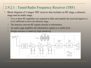
- 1. 1 2.9.2.1 : Tuned Radio Frequency Receiver (TRF) Block diagram of 3-stages TRF receiver that includes an RF stage, a detector stage and an audio stage : Two or three RF amplifiers are required to filter and amplify the received signal to a level sufficient to drive the detector stage. The detector converts RF signals directly to information. An audio stage amplifies the information signals to a usable level Simple and have a relatively high sensitivity
- 2. 2 2.9.2.1 : Tuned Radio Frequency Receiver (TRF) 3 distinct disadvantages : 1. The bandwidth is inconsistent and varies with the center frequency when tuned over a wide range of input frequencies. 2. Instability due to large number of RF amplifiers all tuned to the same center frequency 3. The gains are not uniform over a very wide frequency range.
- 3. 3 2.9.2.2 : Superheterodyne Receiver Heterodyne – to mix two frequencies together in a nonlinear device or to translate one frequency to another using nonlinear mixing. Block diagram of superheterodyne receiver :
- 4. 4 2.9.2.2 : Superheterodyne Receiver 1. RF section Consists of a pre-selector and an amplifier RF amplifier determines the sensitivity of the receiver and a predominant factor in determining the noise figure for the receiver. 2. Mixer/converter section Consists of a radio-frequency oscillator and a mixer. Choice of oscillator depends on the stability and accuracy desired. The shape of the envelope, the bandwidth and the original information contained in the envelope remains unchanged although the carrier and sideband frequencies are translated from RF to IF.
- 5. 5 2.9.2.2 : Superheterodyne Receiver 3. IF section Consists of a series of IF amplifiers and bandpass filters to achieve most of the receiver gain and selectivity. 4. Detector section To convert the IF signals back to the original source information (demodulation).
- 6. 6 2.9.2.2 : Superheterodyne Receiver 5. Audio amplifier section
- 7. 7 2.9.3 : Receiver Operation 2.9.3.1 : Frequency Conversion Frequency conversion in the mixer stage is identical to the frequency conversion in the modulator except that in the receiver, the frequencies are down-converted rather that up-converted. In the mixer, RF signals are combined with the local oscillator frequency Therefore the difference of RF and oscillator frequency is always equal to the IF frequency The adjustment for the center frequency of the pre-selector and the local oscillator frequency are gang-tune (the two adjustments are tied together so that single adjustment will change the center frequency of the pre-selector and at the same time change the local oscillator)
- 8. 8 2.9.3.2 : Frequency Conversion Illustration of the frequency conversion process for an AM broadcast-band superheterodyne receiver using high side injection :
- 9. 9 2.9.3.2 : Frequency Conversion Ex 5-3
- 10. 10 2.9.3.3 : Local oscillator tracking Local oscillator tracking – the ability of the local oscillator in a receiver to oscillate either above or below the selected radio frequency carrier by an amount equal to the intermediate frequency throughout the entire radio frequency band.
- 11. 11 2.9.3.4 : Image frequency Image frequency – any frequency other than the selected radio frequency carrier that will produce a cross-product frequency that is equal to the intermediate frequency if allowed to enter a receiver and mix with the local oscillator. It is equivalent to a second radio frequency that will produce an IF that will interfere with the IF from the desired radio frequency.
- 12. 12 2.9.3.4 : Image frequency The following figure shows the relative frequency spectrum for the RF, IF, local oscillator and image frequencies for a superheterodyne receiver using high side injection. For a radio frequency to produce a cross product equal to IF, it must be displaced from local oscillator frequency by a value equal to the IF. With high side injection, the selected RF is below the local oscillator by amount equal to the IF. Therefore, the image frequency is the radio frequency that is located in the IF frequency above the local oscillator as shown above. (35) IFRFIFloim fffff 2+=+=
- 13. 13 2.9.3.5 : Image frequency rejection ratio Image frequency rejection ratio (IFRR) – a numerical measure of the ability of a pre-selector to reject the image frequency Mathematically expressed as, (36) where ρ= (fim/fRF) – (fRF/fim) Q = quality factor of a pre-selector 22 1 ρQIFRR +=
- 14. 14 Occurs when a receiver picks up the same station at two nearby points on the receiver tuning dial. One point is the desired location, and the other point is called the spurious point. Double spotting
- 15. 15 2.9.3.5 : Image frequency rejection ratio For an AM broadcast-band superheterodyne receiver with IF, RF, and local oscillator frequencies of 455 kHz, 600 kHz, and 1055 kHz, respectively. Determine: a. Image Frequency b. IFRR for a preselector Q of 100
- 16. 16 2.9.4 : Double Conversion Receivers For good image rejection, relatively high IF is desired. However, for a high gain selective amplifiers that are stable, a low IF is necessary. The 1st IF is a relatively high frequency for good image rejection. The 2nd IF is a relatively low frequency for good selectivity and easy amplification.
- 17. Inductive Coupling Inductive or transformer coupling is the most common techniques used for coupling IF amplifiers. 17
- 18. Automatic Gain Control Circuits AGC circuits compensates for minor variations in the received RF signal level. 18
- 19. Squelch Circuits The purpose of a squelch circuit is to quiet a receiver in the absence of a received signal. 19
- 20. 20 2.9.5 : Net Receiver Gain Net receiver gain is simply the ratio of the demodulator signal level at the output of the receiver to the RF signal level at the input to the receiver. In essence, net receiver gain is the dB sum of all gains to the receiver minus the dB sum of all losses. Gains and losses found in a typical radio receiver :
- 22. Electromagnetic Waves An electromagnetic wave propagating through space consists of electric and magnetic fields, perpendicular both to each other and to the direction of travel of the wave. The fields vary together, both in time and in space, and there is a definite ratio between the electric field intensity and the magnetic field intensity.
- 23. Power Density The amount of power that flows through each square meter of a surface perpendicular to the direction of travel.
- 24. Plane and Spherical Waves Conceptually, the simplest source of electromagnetic waves would be a point in space. Waves would radiate equally from this source in all directions. A wavefront is a surface on which all the waves have the same phase, would be the surface of the sphere. Such a source, called an isotropic radiator. Polarization The polarization of a plane wave is simply the direction of its electric field vector.
- 25. Free-Space Propagation Free-space Path Loss It is often defined as the loss incurred by an electromagnetic wave as it propagates in a straight line through a vacuum with no absorption or reflection of energy from nearby objects.
- 26. Transmitting Antenna Gain Until now, we have been assuming an isotropic antenna, that is, one that radiates equally in all directions. Many practical antennas are designed to radiate more power in some directions than others. They are said to have gain in those directions in which the most power is radiated.
- 27. Effective Isotropic Radiated Power (EIRP) is the equivalent power that an isotropic antenna would have to radiate to achieve the same power density in the chosen direction at a given point as another antenna.
- 28. Receiving Antenna Gain The power extracted from a wave by a receiving antenna ought to depend both on its physical size and on its gain.
- 29. Reflection Electromagnetic reflection occurs when an incident wave strikes a boundary of two media and some or all of the incident power does not enter the second material.
- 31. Refraction is sometimes referred to as the bending of the radio- wave path. However, the ray does not actually bend. Electromagnetic refraction is actually the changing of direction of an electromagnetic ray as it passes obliquely from one medium to another with different velocities of propagation.
- 34. Diffraction is defined as the modulation or redistribution of energy within a wavefront when it passes near the edge of an opaque object. Huygens’s Principle states that every point on a given spherical wavefront can be considered as a secondary point source of electromagnetic waves from which other secondary wave (wavelets) are radiated outward.
Hinweis der Redaktion
- If a sphere were drawn at any distance from the source and concentric with it, all the energy from the source would pass through the surface of the sphere. Since no energy would be absorbed by free space, this would be true for any distance, no matter how large. However, the energy would be spread over a larger surface as the distance from the source increased.