Fundamentals of Transport Phenomena ChE 715
•
0 gefällt mir•111 views

Fundamentals of Transport Phenomena ChE 715

Empfohlen
Weitere ähnliche Inhalte
Was ist angesagt?
Was ist angesagt? (19)
Andere mochten auch
Andere mochten auch (14)
Ähnlich wie Fundamentals of Transport Phenomena ChE 715
Ähnlich wie Fundamentals of Transport Phenomena ChE 715 (20)
Kürzlich hochgeladen
Kürzlich hochgeladen (20)
Fundamentals of Transport Phenomena ChE 715
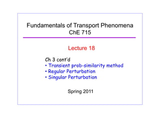
- 1. Fundamentals of Transport Phenomena ChE 715 Lecture 18 Ch 3 cont’d • Transient prob-similarity method R l P t b ti• Regular Perturbation • Singular Perturbation Spring 2011
- 2. Characteristic time scales Two relevant approximations for time dependent problems SECTION 3.4 • Quasi-steady state approximation (QSSA): At “long” times, neglect time derivative(s). • “Penetration” approximation: At “short” times, assume that certain boundaries are far away from the perturbationare far away from the perturbation. Time for concentration (diffusion) or temperature (conduction) propagation over distance L:propagation over distance L: tD ~ L2 Di ; tC ~ L2 α α ≡ k ρC ⎛ ⎝ ⎜ ⎞ ⎠ ⎟. Di α ρCp⎝ ⎠
- 3. Characteristic time scales: membrane pore C1(t); C2(t); volume V (well-mixed) volume V (well-mixed) In the pore: C(x,t) x = 0 x = Lx 0 x L Initial conditions (I.C.’s): C1(0) = KC0 (the perturbation) C (0) = 0C2(0) = 0 C(x,0) = 0
- 4. Characteristic time scales: membrane pore C1(t); C2(t);1 volume V (well-mixed) 2 volume V (well-mixed) In the pore: C(x,t) x = 0 x = Lx = 0 x = L Develop solutions for the QSSA and penetration regimes.p Q p g
- 5. Characteristic time scales: membrane pore C1(t); C2(t); volume V (well-mixed) volume V (well-mixed) In the pore: C(x,t) x = 0 x = L Generally speaking, what is the essence of the QSSA?
- 6. Membrane pore example: QSSA solution 2 2 0; C C D t x ∂ ∂ ∂ ∂ = ≈ 1 2 1( , ) (t) + [ ( ) - ( )] x C x t KC K C t C t L = C1(t) C2(t) C A Bx= + L What BCs have we used? C1(t) 2( ) 1 20, ( ); , ( )x C KC t x L C KC t= = = =1 1 00 ; (0)x x dC V AN C C dt = = − = ( )1 2 x x C C N J DK L − = ≈ From solution of C(x,t) 0 ( )/0 1( ) 1 ; 2 2 tC LV C t e KAD τ τ− = + = How? 1 1 2[ ] dC ADK C C dt LV = − − x = 0 x = L 2 2; (0) 0x x L dC V AN C dt = = − = C dt LV 1 1 0 2 [ / 2] dC ADK dt C C LV = − − 2 1dC dC V V dt dt = − ( )0 2 ( ) 1 2 C C t e τ− = − Integrate, and use BC
- 7. Membrane pore example: QSSA solution (cont.) When is the QSSA justified for this problem? 1. From scaling analysis, the time is well beyond the penetration regime: t >> L2/D 2. We also need the following (membrane vol << external vol): 2 2 1 L ALK D Vτ = <<
- 8. Membrane pore example: penetration solution C1(t); l V C2(t); l Vvolume V (well-mixed) volume V (well-mixed) In the pore: C(x,t) x = 0 x = L Clearly, “short” times means that t << L2/D In this regime, the length of the pore is semi-infinite!
- 9. Membrane pore example: penetration solution Solution of PDE’s by the Similarity Method ∂C = D ∂2 C ; SECTION 3.5 ∂t D ∂x2 ; C(0,t) = C0 ; C(∞,t) = C(x,0) = 0. ∂C ∂t = ∂η ∂t dC dη = − x ′g g2 dC dη = − η ′g g dC dη ; Propose a substitution variable, η = x/g(t): ∂t ∂t dη g dη g dη ∂2 C ∂x2 = 1 g2 d2 C dη2 ; d2 C dη2 + ηg ′g D dC dη = 0. Essence of the similarity method: must be a constantg ′g
- 10. Membrane pore example: penetration solution let g ′g D = a; d2 C dC 0 dη2 + aη dη = 0 let Y = dC d ; ′Y + aηY = 0. dη η Apply the integrating factor method: Y exp aη2 2( )= constant ≡ A; dC d = Aexp −aη2 2( ); let a = 2. dη p η( ) 00 (0)(0, ) C CC t C= ⇒ = BC ( , ) ( ,0) 0 ( ) 0CC t C x∞ = ⇒ ∞= = BCs:
- 11. Membrane pore example: penetration solution Solution of PDE’s by the Similarity Method (cont.) C(η) C0 =1− 2 π e−s2 ds0 η ∫ ≡ erfc η =1− erf η. Apply B.C.’s and solve: η η 0 8 1 0 0.6 0.8 0.2 0.4 0 0 0.5 1 1.5 2 η
- 12. Membrane pore example: penetration solution Solution of PDE’s by the Similarity Method (cont.) Not done yet: need to determine g(t): Initial and boundary conditions must be consistent: g ′g = 2D; C(x,0) = C(∞,t) = 0; requires that g(0) = 0. η = x/g(t) g ′g = 1 2 g2 ( )′; g = 4Dt.g C(η) C = erfc x 4DtC0 4Dt
- 13. Regular Perturbation Perturbation: Regular, Singularg g Define small parameter: ε Mathematical Order: O(1) 1 ~ 1 O(1) 15 ~ 10 O(10) O( )ε ~ ε O(ε) ε2 O(ε2)
- 14. Regular Perturbation Solution when ε = 0 has the same h t th l ti hcharacter as the solution when ε 0: Solution: 2 0 1 2 ... n ε ε ε ∞ Θ = Θ + Θ + Θ + = Θ∑0 n n ε = = Θ∑
- 15. Example Problem – Heated Wire Ts = T∞ From Example 2.8-1 2 ; ; / T T r hR r Bi H R k R k ∞− Θ = = = k, Hv (Bih >> 1) v /H R k R k 2 2 1 4 2 V Vr T T R R R H H k h∞ ⎡ ⎤⎛ ⎞ − − +⎢ ⎥⎜ ⎟ ⎝ ⎠⎢ ⎥⎣ ⎦ = 2 1 1T T r∞− − Θ = = + 0 How? 2 / 4 2v nH R k Bi Θ = = + In this case let How? ( )( ) 1k T k a T T∞ ∞= + −⎡ ⎤⎣ ⎦ ( )⎡ ⎤ In this case, let ( )( ) 1vH T H a T T∞ ∞= + −⎡ ⎤⎣ ⎦
- 16. Example Problem – Heated Wire 1 ( ) ( ) 0v d dT rk T H T r dr dr ⎛ ⎞ + =⎜ ⎟ ⎝ ⎠ Ts = T∞ r dr dr⎝ ⎠ ( )T R T= k, Hv BC’s: 0 dT;( )T R T∞BC s: 0 0 r r dr = =; Define: 2 2 ; ; / T T H Rr r a H R k R k ε∞ ∞ ∞ ∞ ∞ − Θ = = = ε <<1 (basis for pert method)ε <<1 (basis for pert. method)
- 17. Example Problem – Heated Wire Ts = T∞ 1 ( ) ( ) 0v d dT rk T H T r dr dr ⎛ ⎞ + =⎜ ⎟ ⎝ ⎠ k, Hv ( )( ) 1k T k a T T∞ ∞= + −⎡ ⎤⎣ ⎦ ( )( ) 1vH T H a T T∞ ∞= + −⎡ ⎤⎣ ⎦ 2 2 ; ; / H R a T T r r H kR k R ε∞ ∞ ∞ ∞ ∞ − Θ == = 1 (1 ) (1 ) 0 d d r r dr dr ε ε Θ⎛ ⎞ + Θ + + Θ =⎜ ⎟ ⎝ ⎠ ∞ ∞ ∞ ⎝ ⎠ (1) 0Θ =BC’s: 0 d r Θ =( ) 0 0 r r dr =
- 18. Example Problem – Heated Wire 1 (1 ) (1 ) 0 d d r r dr dr ε ε Θ⎛ ⎞ + Θ + + Θ =⎜ ⎟ ⎝ ⎠ Ts = T∞ (1) 0Θ = k, Hv BC’s: 0 0 d r dr Θ =; 0rdr = 2 0 1 ( )Oε εΘ = Θ + Θ +Solve within O(ε) : ⎡ ⎤⎛ ⎞ Then: ( )2 3 20 1 0 1 1 1 ( ) ( ) d dd r O O r dr dr dr ε ε ε ε ε ⎡ Θ ⎤Θ⎛ ⎞ + Θ + Θ + + +⎜ ⎟⎢ ⎥ ⎝ ⎠⎣ ⎦ ( )2 3 0 11 ( ) 0Oε ε ε+ + Θ + Θ + =
- 19. Example Problem – Heated Wire (1) 0Θ = k H Ts = T∞ BC: k, Hv then: 2 0 1(1) (1) ( ) 0Oε εΘ + Θ + = ( )2 3 1 ( ) 0OΘ Θ ( )2 3 20 1 0 1 1 1 ( ) ( ) d dd r O O r dr dr dr ε ε ε ε ε ⎡ Θ ⎤Θ⎛ ⎞ + Θ + Θ + + +⎜ ⎟⎢ ⎥ ⎝ ⎠⎣ ⎦ 01 1 0 dd Θ⎛ ⎞ ⎜ ⎟ 0dΘ O(1) problem: 0 ?Θ = ; ( )2 3 0 11 ( ) 0Oε ε ε+ + Θ + Θ + = 0 1 0r r dr dr ⎛ ⎞ + =⎜ ⎟ ⎝ ⎠ 0 0 0 r d r dr = Θ =0 (1) 0Θ = ( )2 0 1 ( ) 1 4 r rΘ = − Solving :
- 20. Example Problem – Heated Wire ⎡ ⎤⎛ ⎞k H Ts = T∞ O(ε) problem: 1 ?Θ = 0 1 0 0 1 0 d dd r r dr dr dr ⎡ Θ ⎤Θ⎛ ⎞ Θ + + Θ =⎜ ⎟⎢ ⎥ ⎝ ⎠⎣ ⎦ k, Hv 1 0 0 r d r dr = Θ =1(1) 0Θ = ; 1dΘ solving: 0r= ( )4 1 1 ( ) 1 64 r rΘ = − 0 1 2 d r dr Θ = − solving: 64 and the total ( ) ( )2 4 21 ( ) 1 1 ( )O ε Θsolution is: ( ) ( )2 4 21 ( ) 1 1 ( ) 4 64 r r r O ε εΘ = − + − +
- 21. Example Problem 2 – Regular Perturbation Diffusion and second order reaction (slow) at steady state A B y=0 Inert surfacey=L2 CAo Liq film L t Inert surfacey=L2 1 AVAR k C= − at x=L0AdC dy =BCs: CA=CAO at y=0 Let 2 2 0A A VA d C D R dy + = 2 d C 2 ; x= ; Da= AoA Ao AB kC LC y C L D θ = d2 Θ Θ2 0 2 2 2 0A A A d C D kC dy − = Assume Da <<1 and Da=є dx2 −εΘ2 = 0; Θ(0) =1; ′Θ (1) = 0. 2 3 1 2( ) ( ) ( ) ( ) ( )ox x x x Oε ε εΘ = Θ + Θ + Θ +
- 22. Example Problem 2 – Regular Perturbation Example: Diffusion and second order reaction (slow) at steady state. d2 Θ dx2 −εΘ2 = 0; Θ(0) =1; ′Θ (1) = 0. Θ2 = Θ0 +εΘ1 +ε2 Θ2 + O(ε3 )( ) 2 = Θ 2 + 2εΘ Θ +ε2 Θ 2 + 2Θ Θ( )+O(ε3 ) O(1) problem: 2 = Θ0 + 2εΘ0Θ1 +ε2 Θ1 + 2Θ0Θ2( )+O(ε3 ) d2 Θ0 dx2 = 0; Θ0 (0) =1; Θ0 ′(1) = 0;0 ( ) ; 0 ( ) ; Θ0 (x) =1
- 23. Example Problem 2 – Regular Perturbation Example: Second order reaction (slow) d2 Θ1 dx2 =Θ0 2 =1; ′ O(ε) problem: Θ1(0) = 0; Θ1 ′(1) = 0; Θ1(x) = x2 2 − x. d2 Θ2 d 2 = 2Θ0Θ1 = x2 − 2x; O(ε2) problem: dx2 0 1 ; Θ2 (0) = 0; Θ2 ′(1) = 0; Θ ( ) x4 x3 2 Θ2 (x) = x 12 − x 3 + 2 3 x.
- 24. Example Problem 2 – Regular Perturbation Example: Second order reaction (slow) ⎛ ⎞ ⎛ ⎞2 3 4 2 32 ( ) 1 ( ) 2 3 3 12 x x x x x x Oε ε ε ⎛ ⎞ ⎛ ⎞ Θ = − − + − + +⎜ ⎟ ⎜ ⎟ ⎝ ⎠ ⎝ ⎠ 1 0.95 1 ε = 0.1 0.9 ε = 0.2( )xΘ 0.85 ε = 0.5 0.8 0 0.2 0.4 0.6 0.8 1 Position, x
- 25. Example Problem – Singular Perturbation CA(R) = Co R 2 1k R RA = k1CA R r 1 A k R Da D = >> 1 (fast reaction) 1 CA/C0 0 0 1 r/R 1 - ñ01
- 26. Example Problem – Singular Perturbation CA(R) = Co R 1C r RA = k1CA R r 1 0 ; ;AC r r Da C R ε − Θ = = = (1) 1Θ =BC’s: 0 d r Θ =;0 d d r ε Θ⎛ ⎞ − Θ =⎜ ⎟ ⎝ ⎠ 0 0 r r dr = r dr dr ⎜ ⎟ ⎝ ⎠ (trivial solution)ε = 0 Θ = 0 Define: ( )1 b rξ ε≡ − (b < 0)
- 27. Example Problem – Singular Perturbation CA(R) = Co R ( )1 b rξ ε≡ − 1 b r ξε − = − RA = k1CA R r b dr dε ξ− = − bd d dr d ε ξ Θ Θ = − 2 2 2 2 2 bd d dr d ε ξ Θ Θ = dr dξ dr dξ 2 0 d dε ε Θ Θ + Θ = Replacing in the d d l 2 0 dr r dr ε + − Θ =expanded original eq. 2 1b d dε + Θ Θ We obtain: 2 1 2 0 1 b b d d d d ε ε ξ ξε ξ + − Θ Θ − − Θ = −
- 28. Example Problem – Singular Perturbation CA(R) = Co R First term (Diffusion in a slab: O(1) RA = k1CA R r 2 1/ 2 0 d dεΘ Θ − − Θ = Set: b = -1/2 2 1/ 2 0 1d dξ ξε ξ Θ − 1/2 3/2 0 1 2 ( )Oε ε εΘ = Θ + Θ + Θ + 21 1 ( ) ..... x 0 1 x O x for= + + + → Replacing: 0 1 2 ( ) 2 2 d dΘ Θ 1/2 1/2 1 1 ( ) ... 1 Oξε ε ξε = + + + − ( ) 1 f x− 1/20 1 2 ... d d d d ε ξ ξ Θ Θ + + 1/ 2 0dΘ ξ 1/ 2 0 ... d ε ξ − − ( )1/2 0 1 ... 0ε− Θ + Θ + =
- 29. Example Problem – Singular Perturbation CA(R) = Co R 2 1/2 1/2 1/2 1/20 01 1 2 [1 ( )][ ] d dd d O d d d d ε ε ξε ε ε ξ ξ ξ ξ Θ ΘΘ Θ + − + + + RA = k1CA R r 1/2 0 1 ( ) 0 d d d d O ξ ξ ξ ξ ε ε− Θ − Θ + = BC’s: 2 d Θ O(1) problem: (0) 1Θ =2 0 02 0 d dξ Θ − Θ = Other BC: dΘ0 (1) 0 d dξ Θ = (?) NO! because BL doesn’t extend to cylindrical center
- 30. Example Problem – Singular Perturbation CA(R) = Co R 2 0 02 0 d dξ Θ − Θ = RA = k1CA R r BC’s: dξ (0) 1Θ = New BC: ( ) 0Θ ∞ = Solving: 0 e ξ− Θ = O(ε1/2) problem: 2 01 0 dd ΘΘ + + Θ BC’s: 1(0) 0Θ =01 12 0 d dξ ξ + + Θ = BC s: 1( ) 0Θ ∞ = e ξ ξ − 1 2 eξ Θ =Solving: