1. Tutorial: Survival Analysis in Stata
In this tutorial, we use data from the Digitalis Investigation Group (DIG). Recall that the DIG trial
was a was a randomized, double-blind, multicenter trial designed to examine the safety and
efficacy of Digoxin in treating patients with congestive heart failure. In this trial, patients were
randomized to either Digoxin or placebo. The log-rank test was used to compare overall
mortality between the two groups.
To begin, open the dig.dta data set. Before we can do any analyses, we must first tell Stata that
we are working with survival data (analogous to how we had to svyset our data and tell Stata
that we were working with survey data). You can do this using the stset command. The
command for this dataset is stset deathday, failure(death==1). This command tells Stata that
our time-to-death variable is deathday; and a value of 1 for the death variable means that
person died while any other value (in this case 0) means that person was censored. For survival
data, we need at least two variables: 1) a variable for the time to the event and 2) a variable to
indicate if the observation is censored or not.
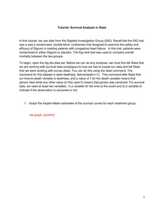
1. Graph the Kaplan-Meier estimates of the survival curves for each treatment group.
.sts graph, by(trtmt)
1

2. Kaplan-Meier survival estimates
1.00
0.75
0.50
0.25
0.00
0 500 1000 1500 2000
analysis time
trtmt = 0 trtmt = 1
Note: you can also list the values of the survival function using the sts list, by(trtmt)
command.
2. In the New England of Journal paper (see handout NEJM_DIG), the authors plotted 1 –
S(t) in Figure 1. Graph 1 – S(t) for each treatment group.
sts graph, failure by(trtmt)
2

3. Kaplan-Meier failure estimates
1.00
0.75
0.50
0.25
0.00
0 500 1000 1500 2000
analysis time
trtmt = 0 trtmt = 1
3. Conduct a log-rank test at the 0.05 level of significance to test the hypothesis that the
survival distribution is the same in the two treatment groups. Use the following
command: sts test trtmt, logrank
a. What are your null and alternative hypotheses?
The null hypothesis is that the two groups have same distribution of survival
times. The alternative is that they do not.
b. What is the value of your test statistic?
0.00
c. What distribution does your test statistic have under the null hypothesis?
Chi-squared distribution with 1 degree of freedom
d. What is your p-value?
0.9616. Note: using all 6800 observation yields a p-value of 0.8013. This is the p-
value the authors reported in Figure 1.
3

4. e. What is your conclusion?
Since our p-value is greater than 0.05, we fail to reject the null hypothesis. Thus,
we conclude that we do not have evidence that the distribution of survival times
is different between the Digoxin group and the placebo group.
4