This ppt. is about what Hyperbolic functions and curves are and where we use them in daily life.

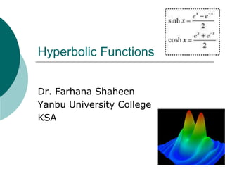
1. Hyperbolic Functions
Dr. Farhana Shaheen
Yanbu University College
KSA

2. Hyperbolic Functions
 Vincenzo Riccati
 (1707 - 1775) is
given credit for
introducing the
hyperbolic functions.
Hyperbolic functions are very useful
in both mathematics and physics.

3. The hyperbolic functions are:
Hyperbolic sine:
Hyperbolic cosine

4. Equilateral hyperbola
 x = coshα , y = sinhα
 x2 – y2= cosh2 α - sinh2 α = 1.

5. GRAPHS OF HYPERBOLIC
FUNCTIONS
 y = sinh x
 y = cosh x

6. Graphs of cosh and sinh functions

7. The St. Louis arch is in the shape of a
hyperbolic cosine.

8. Hyperbolic Curves

9. y = cosh x
 The curve formed by a hanging
necklace is called a catenary. Its
shape follows the curve of
y = cosh x.

10. Catenary Curve
 The curve described by a uniform, flexible
chain hanging under the influence of
gravity is called a catenary curve. This
is the familiar curve of a electric wire
hanging between two telephone poles. In
architecture, an inverted catenary curve
is often used to create domed ceilings.
This shape provides an amazing amount
of structural stability as attested by fact
that many of ancient structures like the
pantheon of Rome which employed the
catenary in their design are still standing.

11. Catenary Curve
 The curve is described by a
COSH(theta) function

12. Example of non-catenary curves

13. Sinh graphs

14. Graphs of tanh and coth functions
 y = tanh x
 y = coth x

15. Graphs of sinh, cosh, and tanh

16. Graphs of sech and csch functions
 y = sech x
 y = csch x

17.  Useful relations


 Hence:
 1 - (tanh x)2 = (sech x)2.





18. RELATIONSHIPS OF HYPERBOLIC
FUNCTIONS
 tanh x = sinh x/cosh x
 coth x = 1/tanh x = cosh x/sinh x
 sech x = 1/cosh x
 csch x = 1/sinh x
 cosh2x - sinh2x = 1
 sech2x + tanh2x = 1
 coth2x - csch2x = 1

19.  The following list shows the
principal values of the inverse
hyperbolic functions expressed in
terms of logarithmic functions which
are taken as real valued.

20.  sinh-1 x = ln (x + ) -∞ < x < ∞
 cosh-1 x = ln (x + ) x≥1
 [cosh-1 x > 0 is principal value]
 tanh-1x = ½ln((1 + x)/(1 - x)) -1 < x
<1
 coth-1 x = ½ln((x + 1)/(x - 1)) x>1
or x < -1
 sech-1 x = ln ( 1/x + )
 0 < x ≤ 1 [sech-1 a; > 0 is principal
value]
 csch-1 x = ln(1/x + ) x≠0

21. Hyperbolic Formulas for Integration
du 1 u 2 2
sinh C or ln ( u u a )
2 2
a u a
du 1 u 2 2
cosh C or ln ( u u a )
2 2
u a a
du 1 1 u 1 a u
2 2
tanh C,u a or ln C, u a
a u a a 2a a u

22. Hyperbolic Formulas for Integration
2 2
du 1 1 u 1 a a u
sec h C or ln ( ) C,0 u a
2 2
u a u a a a u
RELATIONSHIPS OF HYPERBOLIC FUNCTIONS
2 2
du 1 1 u 1 a a u
csc h C or ln ( ) C, u 0.
2 2
u a u a a a u

23.  The hyperbolic functions share many properties with
the corresponding circular functions. In fact, just as
the circle can be represented parametrically by
 x = a cos t
 y = a sin t,
 a rectangular hyperbola (or, more specifically, its
right branch) can be analogously represented by
 x = a cosh t
 y = a sinh t
 where cosh t is the hyperbolic cosine and sinh t is
the hyperbolic sine.

24.  Just as the points (cos t, sin t) form
a circle with a unit radius, the
points (cosh t, sinh t) form the right
half of the equilateral hyperbola.

26. Animated plot of the trigonometric
(circular) and hyperbolic functions
 In red, curve of equation
x² + y² = 1 (unit circle),
and in blue,
x² - y² = 1 (equilateral hyperbola),
with the points (cos(θ),sin(θ)) and
(1,tan(θ)) in red and
(cosh(θ),sinh(θ)) and (1,tanh(θ)) in
blue.

27. Animation of hyperbolic functions

28. Applications of Hyperbolic functions
 Hyperbolic functions occur in the
solutions of some important linear
differential equations, for example
the equation defining a catenary,
and Laplace's equation in Cartesian
coordinates. The latter is important
in many areas of physics, including
electromagnetic theory, heat
transfer, fluid dynamics, and special
relativity.

29.  The hyperbolic functions arise in many
problems of mathematics and
mathematical physics in which integrals
involving a x arise (whereas the
2 2
circular functions involve a x 2 2
).
 For instance, the hyperbolic sine
arises in the gravitational potential of a
cylinder and the calculation of the Roche
limit. The hyperbolic cosine function is
the shape of a hanging cable (the so-
called catenary).

30.  The hyperbolic tangent arises in the
calculation and rapidity of special
relativity. All three appear in the
Schwarzschild metric using external
isotropic Kruskal coordinates in general
relativity. The hyperbolic secant arises
in the profile of a laminar jet. The
hyperbolic cotangent arises in the
Langevin function for magnetic
polarization.

31. Derivatives of Hyperbolic Functions
 d/dx(sinh(x)) = cosh(x)
 d/dx(cosh(x)) = sinh(x)
 d/dx(tanh(x)) = sech2(x)

32. Integrals of Hyperbolic Functions
 ∫ sinh(x)dx = cosh(x) + c
 ∫ cosh(x)dx = sinh(x) + c.
 ∫ tanh(x)dx = ln(cosh x) + c.

33. Example :
Find d/dx (sinh2(3x))
Sol: Using the chain rule,
we have:
d/dx (sinh2(3x))
= 2 sinh(3x) d/dx (sinh(3x))
= 6 sinh(3x) cosh(3x)

34. Inverse hyperbolic functions
 d (sinh−1 (x)) = 1
2
dx 1 x
d 1
 (cosh−1 (x)) = 2
dx x 1
d 1
(tanh−1 (x)) = 2
dx 1 x

35. Curves on Roller Coaster Bridge

37. Masjid in Kazkhistan

38. Fatima masjid in Kuwait

39. Kul Sharif Masjid in Russia

40. Masjid in Georgia

41. Great Masjid in China

42. Thank You

44. Animation of a Hypotrochoid

45. Complex Sinh.jpg