1. Informatica 31 (2007) 249-268 249
Supervised Machine Learning: A Review of Classification
Techniques
S. B. Kotsiantis
Department of Computer Science and Technology
University of Peloponnese, Greece
End of Karaiskaki, 22100 , Tripolis GR.
Tel: +30 2710 372164
Fax: +30 2710 372160
E-mail: sotos@math.upatras.gr
Overview paper
Keywords: classifiers, data mining techniques, intelligent data analysis, learning algorithms
Received: July 16, 2007
Supervised machine learning is the search for algorithms that reason from externally supplied instances
to produce general hypotheses, which then make predictions about future instances. In other words, the
goal of supervised learning is to build a concise model of the distribution of class labels in terms of
predictor features. The resulting classifier is then used to assign class labels to the testing instances
where the values of the predictor features are known, but the value of the class label is unknown. This
paper describes various supervised machine learning classification techniques. Of course, a single
article cannot be a complete review of all supervised machine learning classification algorithms (also
known induction classification algorithms), yet we hope that the references cited will cover the major
theoretical issues, guiding the researcher in interesting research directions and suggesting possible bias
combinations that have yet to be explored.
Povzetek: Podan je pregled metod strojnega učenja.
1 Introduction
There are several applications for Machine Learning Numerous ML applications involve tasks that can be
(ML), the most significant of which is data mining. set up as supervised. In the present paper, we have
People are often prone to making mistakes during concentrated on the techniques necessary to do this. In
analyses or, possibly, when trying to establish particular, this work is concerned with classification
relationships between multiple features. This makes it problems in which the output of instances admits only
difficult for them to find solutions to certain problems. discrete, unordered values.
Machine learning can often be successfully applied to
these problems, improving the efficiency of systems and
the designs of machines.
Every instance in any dataset used by machine learning
algorithms is represented using the same set of features.
The features may be continuous, categorical or binary. If
instances are given with known labels (the corresponding
correct outputs) then the learning is called supervised
(see Table 1), in contrast to unsupervised learning, where Table 1. Instances with known labels (the corresponding
instances are unlabeled. By applying these unsupervised correct outputs)
(clustering) algorithms, researchers hope to discover
unknown, but useful, classes of items (Jain et al., 1999). We have limited our references to recent refereed
Another kind of machine learning is reinforcement journals, published books and conferences. In addition,
learning (Barto & Sutton, 1997). The training we have added some references regarding the original
information provided to the learning system by the work that started the particular line of research under
environment (external trainer) is in the form of a scalar discussion. A brief review of what ML includes can be
reinforcement signal that constitutes a measure of how found in (Dutton & Conroy, 1996). De Mantaras and
well the system operates. The learner is not told which Armengol (1998) also presented a historical survey of
actions to take, but rather must discover which actions logic and instance based learning classifiers. The reader
yield the best reward, by trying each action in turn. should be cautioned that a single article cannot be a

2. 250 Informatica 31 (2007) 249–268 S.B. Kotsiantis
comprehensive review of all classification learning The second step is the data preparation and data pre-
algorithms. Instead, our goal has been to provide a processiong. Depending on the circumstances,
representative sample of existing lines of research in researchers have a number of methods to choose from to
each learning technique. In each of our listed areas, there handle missing data (Batista & Monard, 2003). Hodge &
are many other papers that more comprehensively detail Austin (2004) have recently introduced a survey of
relevant work. contemporary techniques for outlier (noise) detection.
Our next section covers wide-ranging issues of These researchers have identified the techniques’
supervised machine learning such as data pre-processing advantages and disadvantages. Instance selection is not
and feature selection. Logical/Symbolic techniques are only used to handle noise but to cope with the
described in section 3, whereas perceptron-based infeasibility of learning from very large datasets.
techniques are analyzed in section 4. Statistical Instance selection in these datasets is an optimization
techniques for ML are covered in section 5. Section 6 problem that attempts to maintain the mining quality
deals with instance based learners, while Section 7 deals while minimizing the sample size (Liu and Motoda,
with the newest supervised ML technique—Support 2001). It reduces data and enables a data mining
Vector Machines (SVMs). In section 8, some general algorithm to function and work effectively with very
directions are given about classifier selection. Finally, the large datasets. There is a variety of procedures for
last section concludes this work. sampling instances from a large dataset (Reinartz, 2002).
Feature subset selection is the process of identifying
and removing as many irrelevant and redundant features
2 General issues of supervised as possible (Yu & Liu, 2004). This reduces the
dimensionality of the data and enables data mining
learning algorithms algorithms to operate faster and more effectively. The
Inductive machine learning is the process of learning fact that many features depend on one another often
a set of rules from instances (examples in a training set), unduly influences the accuracy of supervised ML
or more generally speaking, creating a classifier that can classification models. This problem can be addressed by
be used to generalize from new instances. The process of constructing new features from the basic feature set
applying supervised ML to a real-world problem is (Markovitch & Rosenstein, 2002). This technique is
described in Figure 1. called feature construction/transformation. These newly
generated features may lead to the creation of more
Problem concise and accurate classifiers. In addition, the
discovery of meaningful features contributes to better
Identification
comprehensibility of the produced classifier, and a better
of required understanding of the learned concept.
data
2.1 Algorithm selection
Data pre-processing
The choice of which specific learning algorithm we
Definition of
should use is a critical step. Once preliminary testing is
training set judged to be satisfactory, the classifier (mapping from
unlabeled instances to classes) is available for routine
Algorithm use. The classifier’s evaluation is most often based on
selection prediction accuracy (the percentage of correct prediction
divided by the total number of predictions). There are at
Parameter tuning Training least three techniques which are used to calculate a
Evaluation
classifier’s accuracy. One technique is to split the
with test set training set by using two-thirds for training and the other
third for estimating performance. In another technique,
No Yes
OK? Classifier known as cross-validation, the training set is divided into
mutually exclusive and equal-sized subsets and for each
subset the classifier is trained on the union of all the
Figure 1. The process of supervised ML
other subsets. The average of the error rate of each subset
is therefore an estimate of the error rate of the classifier.
The first step is collecting the dataset. If a requisite
Leave-one-out validation is a special case of cross
expert is available, then s/he could suggest which fields validation. All test subsets consist of a single instance.
(attributes, features) are the most informative. If not, then This type of validation is, of course, more expensive
the simplest method is that of “brute-force,” which
computationally, but useful when the most accurate
means measuring everything available in the hope that estimate of a classifier’s error rate is required.
the right (informative, relevant) features can be isolated. If the error rate evaluation is unsatisfactory, we must
However, a dataset collected by the “brute-force” method
return to a previous stage of the supervised ML process
is not directly suitable for induction. It contains in most (as detailed in Figure 1). A variety of factors must be
cases noise and missing feature values, and therefore examined: perhaps relevant features for the problem are
requires significant pre-processing (Zhang et al., 2002).

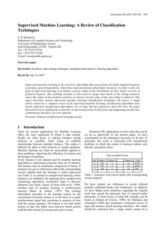
3. SUPERVISED MACHINE LEARNING: A REVIEW OF... Informatica 31 (2007) 249–268 251
not being used, a larger training set is needed, the 3 Logic based algorithms
dimensionality of the problem is too high, the selected
algorithm is inappropriate or parameter tuning is needed.
Another problem could be that the dataset is imbalanced In this section we will concentrate on two groups of
(Japkowicz & Stephen, 2002). logical (symbolic) learning methods: decision trees and
A common method for comparing supervised ML rule-based classifiers.
algorithms is to perform statistical comparisons of the
accuracies of trained classifiers on specific datasets. If 3.1 Decision trees
we have sufficient supply of data, we can sample a Murthy (1998) provided an overview of work in
number of training sets of size N, run the two learning decision trees and a sample of their usefulness to
algorithms on each of them, and estimate the difference newcomers as well as practitioners in the field of
in accuracy for each pair of classifiers on a large test set. machine learning. Thus, in this work, apart from a brief
The average of these differences is an estimate of the description of decision trees, we will refer to some more
expected difference in generalization error across all recent works than those in Murthy’s article as well as
possible training sets of size N, and their variance is an few very important articles that were published earlier.
estimate of the variance of the classifier in the total set. Decision trees are trees that classify instances by sorting
Our next step is to perform paired t-test to check the null them based on feature values. Each node in a decision
hypothesis that the mean difference between the tree represents a feature in an instance to be classified,
classifiers is zero. This test can produce two types of and each branch represents a value that the node can
errors. Type I error is the probability that the test rejects assume. Instances are classified starting at the root node
the null hypothesis incorrectly (i.e. it finds a “significant” and sorted based on their feature values. Figure 2 is an
difference although there is none). Type II error is the example of a decision tree for the training set of Table 2.
probability that the null hypothesis is not rejected, when
there actually is a difference. The test’s Type I error will
be close to the chosen significance level.
at1
In practice, however, we often have only one dataset
of size N and all estimates must be obtained from this
sole dataset. Different training sets are obtained by sub- a1 b1 c1
sampling, and the instances not sampled for training are
used for testing. Unfortunately this violates the
independence assumption necessary for proper at2 No No
significance testing. The consequence of this is that Type
I errors exceed the significance level. This is problematic
a2 b2 c2
because it is important for the researcher to be able to
control Type I errors and know the probability of
incorrectly rejecting the null hypothesis. Several heuristic Yes at3 at4
versions of the t-test have been developed to alleviate
this problem (Dietterich, 1998), (Nadeau and Bengio,
2003). a3 b3 a4 b4
Ideally, we would like the test’s outcome to be
independent of the particular partitioning resulting from Yes No Yes No
the randomization process, because this would make it
much easier to replicate experimental results published in Figure 2. A decision tree
the literature. However, in practice there is always
certain sensitivity to the partitioning used. To measure
replicability we need to repeat the same test several times at1 at2 at3 at4 Class
on the same data with different random partitionings — a1 a2 a3 a4 Yes
usually ten repetitions— and count how often the a1 a2 a3 b4 Yes
outcome is the same (Bouckaert, 2003). a1 b2 a3 a4 Yes
Supervised classification is one of the tasks most a1 b2 b3 b4 No
frequently carried out by so-called Intelligent Systems. a1 c2 a3 a4 Yes
Thus, a large number of techniques have been developed a1 c2 a3 b4 No
based on Artificial Intelligence (Logical/Symbolic b1 b2 b3 b4 No
techniques), Perceptron-based techniques and Statistics c1 b2 b3 b4 No
(Bayesian Networks, Instance-based techniques). In next Table 2. Training Set
sections, we will focus on the most important supervised
machine learning techniques, starting with Using the decision tree depicted in Figure 2 as an
logical/symbolic algorithms. example, the instance 〈at1 = a1, at2 = b2, at3 = a3, at4 =
b4〉 would sort to the nodes: at1, at2, and finally at3,
which would classify the instance as being positive

4. 252 Informatica 31 (2007) 249–268 S.B. Kotsiantis
(represented by the values “Yes”). The problem of no single best pruning method. More details, about not
constructing optimal binary decision trees is an NP- only postprocessing but also about preprocessing of
complete problem and thus theoreticians have searched decision tree algorithms can be fould in (Bruha, 2000).
for efficient heuristics for constructing near-optimal Even though the divide-and-conquer algorithm is
decision trees. quick, efficiency can become important in tasks with
The feature that best divides the training data would hundreds of thousands of instances. The most time-
be the root node of the tree. There are numerous methods consuming aspect is sorting the instances on a numeric
for finding the feature that best divides the training data feature to find the best threshold t. This can be expedited
such as information gain (Hunt et al., 1966) and gini if possible thresholds for a numeric feature are
index (Breiman et al., 1984). While myopic measures determined just once, effectively converting the feature
estimate each attribute independently, ReliefF algorithm to discrete intervals, or if the threshold is determined
(Kononenko, 1994) estimates them in the context of from a subset of the instances. Elomaa & Rousu (1999)
other attributes. However, a majority of studies have stated that the use of binary discretization with C4.5
concluded that there is no single best method (Murthy, needs about the half training time of using C4.5 multi-
1998). Comparison of individual methods may still be splitting. In addition, according to their experiments,
important when deciding which metric should be used in multi-splitting of numerical features does not carry any
a particular dataset. The same procedure is then repeated advantage in prediction accuracy over binary splitting.
on each partition of the divided data, creating sub-trees Decision trees are usually univariate since they use
until the training data is divided into subsets of the same splits based on a single feature at each internal node.
class. Most decision tree algorithms cannot perform well with
Figure 3 presents a general pseudo-code for building problems that require diagonal partitioning. The division
decision trees. of the instance space is orthogonal to the axis of one
variable and parallel to all other axes. Therefore, the
Check for base cases resulting regions after partitioning are all hyper-
For each attribute a rectangles. However, there are a few methods that
Find the feature that best
divides the training data such construct multivariate trees. One example is Zheng’s
as information gain from (1998), who improved the classification accuracy of the
splitting on a decision trees by constructing new binary features with
Let a best be the attribute with the
highest normalized information gain logical operators such as conjunction, negation, and
Create a decision node node that disjunction. In addition, Zheng (2000) created at-least M-
splits on a_best of-N features. For a given instance, the value of an at-
Recurse on the sub-lists obtained by least M-of-N representation is true if at least M of its
splitting on a best and add those
nodes as children of node conditions is true of the instance, otherwise it is false.
Gama and Brazdil (1999) combined a decision tree with
Figure 3. Pseudo-code for building a decision tree a linear discriminant for constructing multivariate
A decision tree, or any learned hypothesis h, is said to decision trees. In this model, new features are computed
overfit training data if another hypothesis h′ exists that as linear combinations of the previous ones.
has a larger error than h when tested on the training data, Decision trees can be significantly more complex
but a smaller error than h when tested on the entire representation for some concepts due to the replication
dataset. There are two common approaches that decision problem. A solution is using an algorithm to implement
tree induction algorithms can use to avoid overfitting complex features at nodes in order to avoid replication.
training data: i) Stop the training algorithm before it Markovitch and Rosenstein (2002) presented the FICUS
reaches a point at which it perfectly fits the training data, construction algorithm, which receives the standard input
ii) Prune the induced decision tree. If the two trees of supervised learning as well as a feature representation
employ the same kind of tests and have the same specification, and uses them to produce a set of generated
prediction accuracy, the one with fewer leaves is usually features. While FICUS is similar in some aspects to other
preferred. Breslow & Aha (1997) survey methods of tree feature construction algorithms, its main strength is its
simplification to improve their comprehensibility. generality and flexibility. FICUS was designed to
The most straightforward way of tackling overfitting perform feature generation given any feature
is to pre-prune the decision tree by not allowing it to representation specification complying with its general
grow to its full size. Establishing a non-trivial purpose grammar.
termination criterion such as a threshold test for the The most well-know algorithm in the literature for
feature quality metric can do that. Decision tree building decision trees is the C4.5 (Quinlan, 1993). C4.5
classifiers usually employ post-pruning techniques that is an extension of Quinlan's earlier ID3 algorithm
evaluate the performance of decision trees, as they are (Quinlan, 1979). One of the latest studies that compare
pruned by using a validation set. Any node can be decision trees and other learning algorithms has been
removed and assigned the most common class of the done by (Tjen-Sien Lim et al. 2000). The study shows
training instances that are sorted to it. A comparative that C4.5 has a very good combination of error rate and
study of well-known pruning methods is presented in speed. In 2001, Ruggieri presented an analytic evaluation
(Elomaa, 1999). Elomaa (1999) concluded that there is of the runtime behavior of the C4.5 algorithm, which
highlighted some efficiency improvements. Based on this

5. SUPERVISED MACHINE LEARNING: A REVIEW OF... Informatica 31 (2007) 249–268 253
analytic evaluation, he implemented a more efficient training instances, separates these instances and
version of the algorithm, called EC4.5. He argued that recursively conquers the remaining instances by learning
his implementation computed the same decision trees as more rules, until no instances remain. In Figure 4, a
C4.5 with a performance gain of up to five times. general pseudo-code for rule learners is presented.
C4.5 assumes that the training data fits in memory, The difference between heuristics for rule learning
thus, Gehrke et al. (2000) proposed Rainforest, a and heuristics for decision trees is that the latter evaluate
framework for developing fast and scalable algorithms to the average quality of a number of disjointed sets (one
construct decision trees that gracefully adapt to the for each value of the feature that is tested), while rule
amount of main memory available. It is clear that in most learners only evaluate the quality of the set of instances
decision tree algorithms; a substantial effort is “wasted” that is covered by the candidate rule. More advanced rule
in the building phase on growing portions of the tree that learners differ from this simple pseudo-code mostly by
are subsequently pruned in the pruning phase. Rastogi & adding additional mechanisms to prevent over-fitting of
Shim (2000) proposed PUBLIC, an improved decision the training data, for instance by stopping the
tree classifier that integrates the second “pruning” phase specialization process with the use of a quality measure
with the initial “building” phase. In PUBLIC, a node is or by generalizing overly specialized rules in a separate
not expanded during the building phase, if it is pruning phase (Furnkranz, 1997).
determined that the node will be pruned during the
subsequent pruning phase. On presentation of training examples
Olcay and Onur (2007) show how to parallelize C4.5 training examples:
1. Initialise rule set to a default
algorithm in three ways: (i) feature based, (ii) node based (usually empty, or a rule assigning all
(iii) data based manner. Baik and Bala (2004) presented objects to the most common class).
preliminary work on an agent-based approach for the 2. Initialise examples to either all
available examples or all examples not
distributed learning of decision trees. correctly handled by rule set.
To sum up, one of the most useful characteristics of 3. Repeat
decision trees is their comprehensibility. People can (a) Find best, the best rule with
easily understand why a decision tree classifies an respect to examples.
(b) If such a rule can be found
instance as belonging to a specific class. Since a decision i. Add best to rule set.
tree constitutes a hierarchy of tests, an unknown feature ii. Set examples to all
value during classification is usually dealt with by examples not handled
passing the example down all branches of the node where correctly by rule set.
until no rule best can be found
the unknown feature value was detected, and each branch (for instance, because no
outputs a class distribution. The output is a combination examples remain).
of the different class distributions that sum to 1. The
Figure 4. Pseudocode for rule learners
assumption made in the decision trees is that instances
belonging to different classes have different values in at It is therefore important for a rule induction system
least one of their features. Decision trees tend to perform to generate decision rules that have high predictability or
better when dealing with discrete/categorical features. reliability. These properties are commonly measured by a
function called rule quality. A rule quality measure is
3.2 Learning set of rules needed in both the rule induction and classification
processes such as J-measure (Smyth and Goodman,
1990). In rule induction, a rule quality measure can be
Decision trees can be translated into a set of rules by
used as a criterion in the rule specification and/or
creating a separate rule for each path from the root to a
generalization process. In classification, a rule quality
leaf in the tree (Quinlan, 1993). However, rules can also
value can be associated with each rule to resolve
be directly induced from training data using a variety of
conflicts when multiple rules are satisfied by the example
rule-based algorithms. Furnkranz (1999) provided an
to be classified. An and Cercone (2000) surveyed a
excellent overview of existing work in rule-based
number of statistical and empirical rule quality measures.
methods.
Furnkranz and Flach (2005) provided an analysis of the
Classification rules represent each class by
behavior of separate-and-conquer or covering rule
disjunctive normal form (DNF). A k-DNF expression is
learning algorithms by visualizing their evaluation
of the form: (X1∧X2∧…∧Xn) ∨ (Xn+1∧Xn+2∧…X2n) ∨ …∨ metrics. When using unordered rule sets, conflicts can
(X(k-1)n+1∧X(k-1)n+2∧…∧Xkn), where k is the number of arise between the rules, i.e., two or more rules cover the
disjunctions, n is the number of conjunctions in each same example but predict different classes. Lindgren
disjunction, and Xn is defined over the alphabet X1, X2,…, (2004) has recently given a survey of methods used to
Xj ∪ ~X1, ~X2, …,~Xj. The goal is to construct the solve this type of conflict.
smallest rule-set that is consistent with the training data. RIPPER is a well-known rule-based algorithm
A large number of learned rules is usually a sign that the (Cohen, 1995). It forms rules through a process of
learning algorithm is attempting to “remember” the repeated growing and pruning. During the growing phase
training set, instead of discovering the assumptions that the rules are made more restrictive in order to fit the
govern it. A separate-and-conquer algorithm (covering training data as closely as possible. During the pruning
algorithms) search for a rule that explains a part of its phase, the rules are made less restrictive in order to avoid

6. 254 Informatica 31 (2007) 249–268 S.B. Kotsiantis
overfitting, which can cause poor performance on unseen class. They do this independent of all the other classes in
instances. RIPPER handles multiple classes by ordering the training set. For this reason, for small datasets, it may
them from least to most prevalent and then treating each be better to use a divide-and-conquer algorithm that
in order as a distinct two-class problem. Other considers the entire set at once.
fundamental learning classifiers based on decision rules To sum up, the most useful characteristic of rule-
include the AQ family (Michalski and Chilausky, 1980) based classifiers is their comprehensibility. In addition,
and CN2 (Clark and Niblett, 1989). Bonarini (2000) gave even though some rule-based classifiers can deal with
an overview of fuzzy rule-based classifiers. Fuzzy logic numerical features, some experts propose these features
tries to improve classification and decision support should be discretized before induction, so as to reduce
systems by allowing the use of overlapping class training time and increase classification accuracy (An
definitions. and Cercone, 1999). Classification accuracy of rule
Furnkranz (2001) investigated the use of round robin learning algorithms can be improved by combining
binarization (or pairwise classification) as a technique for features (such as in decision trees) using the background
handling multi-class problems with separate and conquer knowledge of the user (Flach and Lavrac, 2000) or
rule learning algorithms. The round robin binarization automatic feature construction algorithms (Markovitch
transforms a c-class problem into c(c-1)/2 two-class and Rosenstein, 2002).
problems <i,j>, one for each set of classes {i,j}, i= 1 ... c-
1, j = i+1 ...c. The binary classifier for problem <i,j> is 4 Perceptron-based techniques
trained with examples of classes i and j, whereas
examples of classes k ≠ i,j are ignored for this problem. Other well-known algorithms are based on the notion
A crucial point, of course, is determining how to decode of perceptron (Rosenblatt, 1962).
the predictions of the pairwise classifiers for a final
prediction. Furnkranz (2001) implemented a simple 4.1 Single layered perceptrons
voting technique: when classifying a new example, each
of the learned base classifiers determines to which of its A single layered perceptron can be briefly described
two classes the example is more likely to belong to. The as follows:
winner is assigned a point, and in the end, the algorithm If x1 through xn are input feature values and w1
predicts the class that has accumulated the most points. through wn are connection weights/prediction vector
His experimental results show that, in comparison to (typically real numbers in the interval [-1, 1]), then
conventional, ordered or unordered binarization, the perceptron computes the sum of weighted inputs:
round robin approach may yield significant gains in
accuracy without risking a poor performance.
∑xw i i
and output goes through an adjustable threshold:
i
There are numerous other rule-based learning if the sum is above threshold, output is 1; else it is 0.
algorithms. Furnkranz (1999) referred to most of them. The most common way that the perceptron algorithm
The PART algorithm infers rules by repeatedly is used for learning from a batch of training instances is
generating partial decision trees, thus combining the two to run the algorithm repeatedly through the training set
major paradigms for rule generation − creating rules until it finds a prediction vector which is correct on all of
from decision trees and the separate-and-conquer rule- the training set. This prediction rule is then used for
learning technique. Once a partial tree has been build, a predicting the labels on the test set.
single rule is extracted from it and for this reason the WINNOW (Littlestone & Warmuth, 1994) is based
PART algorithm avoids postprocessing (Frank and on the perceptron idea and updates its weights as follows.
Witten, 1998). If prediction value y΄=0 and actual value y=1, then the
For the task of learning binary problems, rules are weights are too low; so, for each feature such that xi=1,
more comprehensible than decision trees because typical wi=wi·α, where α is a number greater than 1, called the
rule-based approaches learn a set of rules for only the promotion parameter. If prediction value y΄= 1 and
positive class. On the other hand, if definitions for actual value y=0, then the weights were too high; so, for
multiple classes are to be learned, the rule-based learner each feature xi = 1, it decreases the corresponding weight
must be run separately for each class separately. For each by setting wi=wi·β, where 0<β<1, called the demotion
individual class a separate rule set is obtained and these parameter. Generally, WINNOW is an example of an
sets may be inconsistent (a particular instance might be exponential update algorithm. The weights of the
assigned multiple classes) or incomplete (no class might relevant features grow exponentially but the weights of
be assigned to a particular instance). These problems can the irrelevant features shrink exponentially. For this
be solved with decision lists (the rules in a rule set are reason, it was experimentally proved (Blum, 1997) that
supposed to be ordered, a rule is only applicable when WINNOW can adapt rapidly to changes in the target
none of the preceding rules are applicable) but with the function (concept drift). A target function (such as user
decision tree approach, they simply do not occur. preferences) is not static in time. In order to enable, for
Moreover, the divide and conquer approach (used by example, a decision tree algorithm to respond to changes,
decision trees) is usually more efficient than the separate it is necessary to decide which old training instances
and conquer approach (used by rule-based algorithms). could be deleted. A number of algorithms similar to
Separate-and-conquer algorithms look at one class at a
time, and try to produce rules that uniquely identify the

7. SUPERVISED MACHINE LEARNING: A REVIEW OF... Informatica 31 (2007) 249–268 255
WINNOW have been developed, such as those by Auer First, the network is trained on a set of paired data to
& Warmuth (1998). determine input-output mapping. The weights of the
Freund & Schapire (1999) created a newer connections between neurons are then fixed and the
algorithm, called voted-perceptron, which stores more network is used to determine the classifications of a new
information during training and then uses this elaborate set of data.
information to generate better predictions about the test During classification the signal at the input units
data. The information it maintains during training is the propagates all the way through the net to determine the
list of all prediction vectors that were generated after activation values at all the output units. Each input unit
each and every mistake. For each such vector, it counts has an activation value that represents some feature
the number of iterations it “survives” until the next external to the net. Then, every input unit sends its
mistake is made; Freund & Schapire refer to this count as activation value to each of the hidden units to which it is
the “weight” of the prediction vector. To calculate a connected. Each of these hidden units calculates its own
prediction the algorithm computes the binary prediction activation value and this signal are then passed on to
of each one of the prediction vectors and combines all output units. The activation value for each receiving unit
these predictions by means of a weighted majority vote. is calculated according to a simple activation function.
The weights used are the survival times described above. The function sums together the contributions of all
To sum up, we have discussed perceptron-like linear sending units, where the contribution of a unit is defined
algorithms with emphasis on their superior time as the weight of the connection between the sending and
complexity when dealing with irrelevant features. This receiving units multiplied by the sending unit's activation
can be a considerable advantage when there are many value. This sum is usually then further modified, for
features, but only a few relevant ones. Generally, all example, by adjusting the activation sum to a value
perceptron-like linear algorithms are anytime online between 0 and 1 and/or by setting the activation value to
algorithms that can produce a useful answer regardless of zero unless a threshold level for that sum is reached.
how long they run (Kivinen, 2002). The longer they run, Generally, properly determining the size of the
the better the result they produce. Finally, perceptron-like hidden layer is a problem, because an underestimate of
methods are binary, and therefore in the case of multi- the number of neurons can lead to poor approximation
class problem one must reduce the problem to a set of and generalization capabilities, while excessive nodes
multiple binary classification problems. can result in overfitting and eventually make the search
for the global optimum more difficult. An excellent
4.2 Multilayered perceptrons argument regarding this topic can be found in (Camargo
& Yoneyama, 2001). Kon & Plaskota (2000) also studied
Perceptrons can only classify linearly separable sets the minimum amount of neurons and the number of
of instances. If a straight line or plane can be drawn to instances necessary to program a given task into feed-
seperate the input instances into their correct categories, forward neural networks.
input instances are linearly separable and the perceptron ANN depends upon three fundamental aspects, input
will find the solution. If the instances are not linearly and activation functions of the unit, network architecture
separable learning will never reach a point where all and the weight of each input connection. Given that the
instances are classified properly. Multilayered first two aspects are fixed, the behavior of the ANN is
Perceptrons (Artificial Neural Networks) have been defined by the current values of the weights. The weights
created to try to solve this problem (Rumelhart et al., of the net to be trained are initially set to random values,
1986). Zhang (2000) provided an overview of existing and then instances of the training set are repeatedly
work in Artificial Neural Networks (ANNs). Thus, in this exposed to the net. The values for the input of an
study, apart from a brief description of the ANNs we will instance are placed on the input units and the output of
mainly refer to some more recent articles. A multi-layer the net is compared with the desired output for this
neural network consists of large number of units instance. Then, all the weights in the net are adjusted
(neurons) joined together in a pattern of connections slightly in the direction that would bring the output
(Figure 5). Units in a net are usually segregated into three values of the net closer to the values for the desired
classes: input units, which receive information to be output. There are several algorithms with which a
processed; output units, where the results of the network can be trained (Neocleous & Schizas, 2002).
processing are found; and units in between known as However, the most well-known and widely used learning
hidden units. Feed-forward ANNs (Figure 5) allow algorithm to estimate the values of the weights is the
signals to travel one way only, from input to output. Back Propagation (BP) algorithm. Generally, BP
algorithm includes the following six steps:
1. Present a training sample to the neural network.
2. Compare the network's output to the desired output
from that sample. Calculate the error in each output
neuron.
3. For each neuron, calculate what the output should
have been, and a scaling factor, how much lower or
Figure 5. Feed-forward ANN higher the output must be adjusted to match the
desired output. This is the local error.

8. 256 Informatica 31 (2007) 249–268 S.B. Kotsiantis
4. Adjust the weights of each neuron to lower the local constructive algorithms, where extra nodes are added as
error. required (Parekh et al. 2000).
5. Assign "blame" for the local error to neurons at the
previous level, giving greater responsibility to 4.3 Radial Basis Function (RBF) networks
neurons connected by stronger weights.
6. Repeat the steps above on the neurons at the ANN learning can be achieved, among others,
previous level, using each one's "blame" as its error. through i) synaptic weight modification, ii) network
With more details, the general rule for updating structure modifications (creating or deleting neurons or
synaptic connections), iii) use of suitable attractors or
weights is: ∆W ji = ηδ j Oi where:
other suitable stable state points, iv) appropriate choice
• η is a positive number (called learning rate), which of activation functions. Since back-propagation training
determines the step size in the gradient descent is a gradient descending process, it may get stuck in local
search. A large value enables back propagation to minima in this weight-space. It is because of this
move faster to the target weight configuration but it possibility that neural network models are characterized
also increases the chance of its never reaching this by high variance and unsteadiness.
target. Radial Basis Function (RBF) networks have been
• Oi is the output computed by neuron i also widely applied in many science and engineering
• δ j = O j (1 − O j )(T j − O j ) for the output neurons, fields (Robert and Howlett, 2001). An RBF network is a
three-layer feedback network, in which each hidden unit
where Tj the wanted output for the neuron j and implements a radial activation function and each output
• δ j = O j (1 − O j )∑ δ kWkj for the internal unit implements a weighted sum of hidden units outputs.
k Its training procedure is usually divided into two stages.
(hidden) neurons First, the centers and widths of the hidden layer are
The back propagation algorithm will have to perform determined by clustering algorithms. Second, the weights
a number of weight modifications before it reaches a connecting the hidden layer with the output layer are
good weight configuration. For n training instances and determined by Singular Value Decomposition (SVD) or
W weights, each repetition/epoch in the learning process Least Mean Squared (LMS) algorithms. The problem of
takes O(nW) time; but in the worst case, the number of selecting the appropriate number of basis functions
epochs can be exponential to the number of inputs. For remains a critical issue for RBF networks. The number of
this reason, neural nets use a number of different basis functions controls the complexity and the
stopping rules to control when training ends. The four generalization ability of RBF networks. RBF networks
most common stopping rules are: i) Stop after a specified with too few basis functions cannot fit the training data
number of epochs, ii) Stop when an error measure adequately due to limited flexibility. On the other hand,
reaches a threshold, iii) Stop when the error measure has those with too many basis functions yield poor
seen no improvement over a certain number of epochs, generalization abilities since they are too flexible and
iv) Stop when the error measure on some of the data that erroneously fit the noise in the training data.
has been sampled from the training data (hold-out set, Even though multilayer neural networks and decision
validation set) is more than a certain amount than the trees are two very different techniques for the purpose of
error measure on the training set (overfitting). classification, some researchers (Eklund & Hoang,
Feed-forward neural networks are usually trained by 2002), (Tjen-Sien Lim et al. 2000) have performed some
the original back propagation algorithm or by some empirical comparative studies. Some of the general
variant. Their greatest problem is that they are too slow conclusions drawn in that work are:
for most applications. One of the approaches to speed up i) neural networks are usually more able to easily
the training rate is to estimate optimal initial weights provide incremental learning than decision trees
(Yam & Chow, 2001). Another method for training (Saad, 1998), even though there are some
multilayered feedforward ANNs is Weight-elimination algorithms for incremental learning of decision
algorithm that automatically derives the appropriate trees such as (Utgoff et al, 1997) and
topology and therefore avoids also the problems with (McSherry, 1999). Incremental decision tree
overfitting (Weigend et al., 1991). Genetic algorithms induction techniques result in frequent tree
have been used to train the weights of neural networks restructuring when the amount of training data
(Siddique and Tokhi, 2001) and to find the architecture is small, with the tree structure maturing as the
of neural networks (Yen and Lu, 2000). There are also data pool becomes larger.
Bayesian methods in existence which attempt to train ii) training time for a neural network is usually
neural networks. Vivarelli & Williams (2001) compare much longer than training time for decision
two Bayesian methods for training neural networks. A trees.
number of other techniques have emerged recently which iii) neural networks usually perform as well as
attempt to improve ANNs training algorithms by decision trees, but seldom better.
changing the architecture of the networks as training
proceeds. These techniques include pruning useless To sum up, ANNs have been applied to many real-
nodes or weights (Castellano et al. 1997), and world problems but still, their most striking disadvantage
is their lack of ability to reason about their output in a

9. SUPERVISED MACHINE LEARNING: A REVIEW OF... Informatica 31 (2007) 249–268 257
way that can be effectively communicated. For this
R=
P (i | X )
=
∏ P ( X | i)
P (i ) P ( X | i )
=
P (i ) r
reason many researchers have tried to address the issue
P ( j | X ) P ( j) P( X | j) P( j)∏ P( X | j)
of improving the comprehensibility of neural networks, r
where the most attractive solution is to extract symbolic Comparing these two probabilities, the larger
rules from trained neural networks. Setiono and Leow probability indicates that the class label value that is
(2000) divided the activation values of relevant hidden more likely to be the actual label (if R>1: predict i else
units into two subintervals and then found the set of predict j). Cestnik et al (1987) first used the Naive Bayes
relevant connections of those relevant units to construct in ML community. Since the Bayes classification
rules. More references can be found in (Zhou, 2004), an algorithm uses a product operation to compute the
excellent survey. However, it is also worth mentioning probabilities P(X, i), it is especially prone to being
that Roy (2000) identified the conflict between the idea unduly impacted by probabilities of 0. This can be
of rule extraction and traditional connectionism. In detail, avoided by using Laplace estimator or m-esimate, by
the idea of rule extraction from a neural network involves adding one to all numerators and adding the number of
certain procedures, specifically the reading of parameters added ones to the denominator (Cestnik, 1990).
from a network, which is not allowed by the traditional The assumption of independence among child nodes
connectionist framework that these neural networks are is clearly almost always wrong and for this reason naive
based on. Bayes classifiers are usually less accurate that other more
sophisticated learning algorithms (such ANNs).
However, Domingos & Pazzani (1997) performed a
5 Statistical learning algorithms large-scale comparison of the naive Bayes classifier with
Conversely to ANNs, statistical approaches are state-of-the-art algorithms for decision tree induction,
characterized by having an explicit underlying instance-based learning, and rule induction on standard
probability model, which provides a probability that an benchmark datasets, and found it to be sometimes
instance belongs in each class, rather than simply a superior to the other learning schemes, even on datasets
classification. Linear discriminant analysis (LDA) and with substantial feature dependencies.
the related Fisher's linear discriminant are simple The basic independent Bayes model has been
methods used in statistics and machine learning to find modified in various ways in attempts to improve its
the linear combination of features which best separate performance. Attempts to overcome the independence
two or more classes of object (Friedman, 1989). LDA assumption are mainly based on adding extra edges to
works when the measurements made on each observation include some of the dependencies between the features,
are continuous quantities. When dealing with categorical for example (Friedman et al. 1997). In this case, the
variables, the equivalent technique is Discriminant network has the limitation that each feature can be
Correspondence Analysis (Mika et al., 1999). related to only one other feature. Semi-naive Bayesian
Maximum entropy is another general technique for classifier is another important attempt to avoid the
estimating probability distributions from data. The over- independence assumption. (Kononenko, 1991), in which
riding principle in maximum entropy is that when attributes are partitioned into groups and it is assumed
nothing is known, the distribution should be as uniform that xi is conditionally independent of xj if and only if
as possible, that is, have maximal entropy. Labeled they are in different groups.
training data is used to derive a set of constraints for the The major advantage of the naive Bayes classifier is
model that characterize the class-specific expectations for its short computational time for training. In addition,
the distribution. Csiszar (1996) provides a good tutorial since the model has the form of a product, it can be
introduction to maximum entropy techniques. converted into a sum through the use of logarithms - with
Bayesian networks are the most well known significant consequent computational advantages. If a
representative of statistical learning algorithms. A feature is numerical, the usual procedure is to discretize
comprehensive book on Bayesian networks is Jensen’s it during data pre-processing (Yang & Webb, 2003),
(1996). Thus, in this study, apart from our brief although a researcher can use the normal distribution to
description of Bayesian networks, we mainly refer to calculate probabilities (Bouckaert, 2004).
more recent works.
5.2 Bayesian Networks
5.1.1 Naive Bayes classifiers
A Bayesian Network (BN) is a graphical model for
Naive Bayesian networks (NB) are very simple probability relationships among a set of variables
Bayesian networks which are composed of directed (features) (see Figure 6). The Bayesian network structure
acyclic graphs with only one parent (representing the S is a directed acyclic graph (DAG) and the nodes in S
unobserved node) and several children (corresponding to are in one-to-one correspondence with the features X.
observed nodes) with a strong assumption of The arcs represent casual influences among the features
independence among child nodes in the context of their while the lack of possible arcs in S encodes conditional
parent (Good, 1950).Thus, the independence model independencies. Moreover, a feature (node) is
(Naive Bayes) is based on estimating (Nilsson, 1965): conditionally independent from its non-descendants
given its parents (X1 is conditionally independent from X2

10. 258 Informatica 31 (2007) 249–268 S.B. Kotsiantis
given X3 if P(X1|X2,X3)=P(X1|X3) for all possible values of Initialize an empty Bayesian network
X1, X2, X3). G containing n nodes (i.e., a BN with n
nodes but no edges)
1. Evaluate the score of G: Score(G)
2. G’ = G
3. for i = 1 to n do
4. for j = 1 to n do
5. if i • j then
6. if there is no edge between the
nodes i and j in G• then
7. Modify G’ by adding an edge between
the nodes i and j in G• such that i
is a parent of j: (i • j)
8. if the resulting G’ is a DAG then
Figure 6. The structure of a Bayes Network 9. if (Score(G’) > Score(G)) then
10. G = G’
Typically, the task of learning a Bayesian network 11. end if
can be divided into two subtasks: initially, the learning of 12. end if
13. end if
the DAG structure of the network, and then the 14. end if
determination of its parameters. Probabilistic parameters 15. G’ = G
are encoded into a set of tables, one for each variable, in 16. end for
the form of local conditional distributions of a variable 17. end for
given its parents. Given the independences encoded into Figure 7. Pseudo-code for training BN
the network, the joint distribution can be reconstructed
by simply multiplying these tables. Within the general A BN structure can be also found by learning the
framework of inducing Bayesian networks, there are two conditional independence relationships among the
scenarios: known structure and unknown structure. features of a dataset. Using a few statistical tests (such as
In the first scenario, the structure of the network is the Chi-squared and mutual information test), one can
given (e.g. by an expert) and assumed to be correct. Once find the conditional independence relationships among
the network structure is fixed, learning the parameters in the features and use these relationships as constraints to
the Conditional Probability Tables (CPT) is usually construct a BN. These algorithms are called CI-based
solved by estimating a locally exponential number of algorithms or constraint-based algorithms. Cowell (2001)
parameters from the data provided (Jensen, 1996). Each has shown that for any structure search procedure based
node in the network has an associated CPT that describes on CI tests, an equivalent procedure based on
the conditional probability distribution of that node given maximizing a score can be specified.
the different values of its parents. A comparison of scoring-based methods and CI-
In spite of the remarkable power of Bayesian based methods is presented in (Heckerman et al., 1999).
Networks, they have an inherent limitation. This is the Both of these approaches have their advantages and
computational difficulty of exploring a previously disadvantages. Generally speaking, the dependency
unknown network. Given a problem described by n analysis approach is more efficient than the search &
features, the number of possible structure hypotheses is scoring approach for sparse networks (networks that are
more than exponential in n. If the structure is unknown, not densely connected). It can also deduce the correct
one approach is to introduce a scoring function (or a structure when the probability distribution of the data
score) that evaluates the “fitness” of networks with satisfies certain assumptions. However, many of these
respect to the training data, and then to search for the algorithms require an exponential number of CI tests and
best network according to this score. Several researchers many high order CI tests (CI tests with large condition-
have shown experimentally that the selection of a single sets). Yet although the search & scoring approach may
good hypothesis using greedy search often yields not find the best structure due to its heuristic nature, it
accurate predictions (Heckerman et al. 1999), works with a wider range of probabilistic models than the
(Chickering, 2002). In Figure 7 there is a pseudo-code dependency analysis approach. Madden (2003) compared
for training BNs. the performance of a number of Bayesian Network
Within the score & search paradigm, another Classifiers. His experiments demonstrated that very
approach uses local search methods in the space of similar classification performance can be achieved by
directed acyclic graphs, where the usual choices for classifiers constructed using the different approaches
defining the elementary modifications (local changes) described above.
that can be applied are arc addition, arc deletion, and arc The most generic learning scenario is when the
reversal. Acid and de Campos (2003) proposed a new structure of the network is unknown and there is missing
local search method, restricted acyclic partially directed data. Friedman & Koller (2003) proposed a new
graphs, which uses a different search space and takes approach for this task and showed how to efficiently
account of the concept of equivalence between network compute a sum over the exponential number of networks
structures. In this way, the number of different that are consistent with a fixed order over networks.
configurations of the search space is reduced, thus Using a suitable version of any of the model types
improving efficiency. mentioned in this review, one can induce a Bayesian
Network from a given training set. A classifier based on
the network and on the given set of features X1,X2, ... Xn,

11. SUPERVISED MACHINE LEARNING: A REVIEW OF... Informatica 31 (2007) 249–268 259
returns the label c, which maximizes the posterior tagged with a classification label, then the value of the
probability p(c | X1, X2, ... Xn). label of an unclassified instance can be determined by
Bayesian multi-nets allow different probabilistic observing the class of its nearest neighbours. The kNN
dependencies for different values of the class node locates the k nearest instances to the query instance and
(Jordan, 1998). This suggests that simple BN classifiers determines its class by identifying the single most
should work better when there is a single underlying frequent class label. In Figure 8, a pseudo-code example
model of the dataset and multi-net classifier should work for the instance base learning methods is illustrated.
better when the underlying relationships among the
features are very different for different classes (Cheng procedure InstanceBaseLearner(Testing
and Greiner, 2001). Instances)
for each testing instance
The most interesting feature of BNs, compared to {
decision trees or neural networks, is most certainly the find the k most nearest instances of
possibility of taking into account prior information about the training set according to a
distance metric
a given problem, in terms of structural relationships Resulting Class= most frequent class
among its features. This prior expertise, or domain label of the k nearest instances
knowledge, about the structure of a Bayesian network }
can take the following forms:
Figure 8. Pseudo-code for instance-based learners
1. Declaring that a node is a root node, i.e., it has no
parents. In general, instances can be considered as points
2. Declaring that a node is a leaf node, i.e., it has no within an n-dimensional instance space where each of the
children. n-dimensions corresponds to one of the n-features that
3. Declaring that a node is a direct cause or direct are used to describe an instance. The absolute position of
effect of another node. the instances within this space is not as significant as the
4. Declaring that a node is not directly connected to relative distance between instances. This relative distance
another node. is determined by using a distance metric. Ideally, the
5. Declaring that two nodes are independent, given a distance metric must minimize the distance between two
condition-set. similarly classified instances, while maximizing the
6. Providing partial nodes ordering, that is, declare that distance between instances of different classes. Many
a node appears earlier than another node in the different metrics have been presented. The most
ordering. significant ones are presented in Table 3.
7. Providing a complete node ordering.
A problem of BN classifiers is that they are not 1/ r
⎛ m r ⎞
suitable for datasets with many features (Cheng et al., Minkowsky: D(x,y)= ⎜ ∑ xi − yi ⎟
2002). The reason for this is that trying to construct a ⎝ i =1 ⎠
very large network is simply not feasible in terms of time m
and space. A final problem is that before the induction,
the numerical features need to be discretized in most
Manhattan: D(x,y)= ∑ x −y i i
i =1
cases. m
Chebychev: D(x,y)= max xi − yi
i =1
6 Instance-based learning 1/ 2
⎛ m 2 ⎞
Another category under the header of statistical Euclidean: D(x,y)= ⎜ ∑ xi − yi ⎟
methods is Instance-based learning. Instance-based ⎝ i =1 ⎠
learning algorithms are lazy-learning algorithms m
xi − yi
(Mitchell, 1997), as they delay the induction or Camberra: D(x,y)= ∑ x +y
generalization process until classification is performed. i =1 i i
Lazy-learning algorithms require less computation time Kendall’s Rank Correlation:
during the training phase than eager-learning algorithms 2 m i −1
(such as decision trees, neural and Bayes nets) but more D(x,y)= 1 − ∑∑ sign( xi − x j ) sign( yi − y j )
m( m − 1) i = j j =1
computation time during the classification process. One
of the most straightforward instance-based learning
Table 3. Approaches to define the distance between
algorithms is the nearest neighbour algorithm. Aha
instances (x and y)
(1997) and De Mantaras and Armengol (1998) presented
a review of instance-based learning classifiers. Thus, in For more accurate results, several algorithms use
this study, apart from a brief description of the nearest weighting schemes that alter the distance measurements
neighbour algorithm, we will refer to some more recent and voting influence of each instance. A survey of
works. weighting schemes is given by (Wettschereck et al.,
k-Nearest Neighbour (kNN) is based on the principle 1997).
that the instances within a dataset will generally exist in The power of kNN has been demonstrated in a
close proximity to other instances that have similar number of real domains, but there are some reservations
properties (Cover and Hart, 1967). If the instances are about the usefulness of kNN, such as: i) they have large

12. 260 Informatica 31 (2007) 249–268 S.B. Kotsiantis
storage requirements, ii) they are sensitive to the choice As we have already mentioned, the major
of the similarity function that is used to compare disadvantage of instance-based classifiers is their large
instances, iii) they lack a principled way to choose k, computational time for classification. A key issue in
except through cross-validation or similar, many applications is to determine which of the available
computationally-expensive technique (Guo et al. 2003). input features should be used in modeling via feature
The choice of k affects the performance of the kNN selection (Yu & Liu, 2004), because it could improve the
algorithm. Consider the following reasons why a k- classification accuracy and scale down the required
nearest neighbour classifier might incorrectly classify a classification time. Furthermore, choosing a more
query instance: suitable distance metric for the specific dataset can
• When noise is present in the locality of the query improve the accuracy of instance-based classifiers.
instance, the noisy instance(s) win the majority vote,
resulting in the incorrect class being predicted. A 7 Support Vector Machines
larger k could solve this problem.
• When the region defining the class, or fragment of Support Vector Machines (SVMs) are the newest
the class, is so small that instances belonging to the supervised machine learning technique (Vapnik, 1995).
class that surrounds the fragment win the majority An excellent survey of SVMs can be found in (Burges,
vote. A smaller k could solve this problem. 1998), and a more recent book is by (Cristianini &
Wettschereck et al. (1997) investigated the behavior Shawe-Taylor, 2000). Thus, in this study apart from a
of the kNN in the presence of noisy instances. The brief description of SVMs we will refer to some more
experiments showed that the performance of kNN was recent works and the landmark that were published
not sensitive to the exact choice of k when k was large. before these works. SVMs revolve around the notion of a
They found that for small values of k, the kNN algorithm “margin”—either side of a hyperplane that separates two
was more robust than the single nearest neighbour data classes. Maximizing the margin and thereby creating
algorithm (1NN) for the majority of large datasets tested. the largest possible distance between the separating
However, the performance of the kNN was inferior to hyperplane and the instances on either side of it has been
that achieved by the 1NN on small datasets (<100 proven to reduce an upper bound on the expected
instances). generalisation error.
Okamoto and Yugami (2003) represented the If the training data is linearly separable, then a pair
expected classification accuracy of k-NN as a function of (w, b) exists such that
domain characteristics including the number of training
instances, the number of relevant and irrelevant
w T xi + b ≥ 1, for all x i ∈ P
attributes, the probability of each attribute, the noise rate w T xi + b ≤ −1, for all xi ∈ N
for each type of noise, and k. They also explored the
with the decision rule given by
behavioral implications of the analyses by presenting the T
effects of domain characteristics on the expected f w ,b (x) = sgn(w x + b) where w is termed the
accuracy of k-NN and on the optimal value of k for weight vector and b the bias (or − b is termed the
artificial domains.
threshold).
The time to classify the query instance is closely
It is easy to show that, when it is possible to linearly
related to the number of stored instances and the number
separate two classes, an optimum separating hyperplane
of features that are used to describe each instance. Thus,
can be found by minimizing the squared norm of the
in order to reduce the number of stored instances,
separating hyperplane. The minimization can be set up as
instance-filtering algorithms have been proposed (Kubat
a convex quadratic programming (QP) problem:
and Cooperson, 2001). Brighton & Mellish (2002) found
1 2
that their ICF algorithm and RT3 algorithm (Wilson & Minimize Φ(w ) = w
w ,b 2 (1)
Martinez, 2000) achieved the highest degree of instance
T
set reduction as well as the retention of classification subject to yi (w xi + b) ≥ 1, i = 1,K, l.
accuracy: they are close to achieving unintrusive storage In the case of linearly separable data, once the
reduction. The degree to which these algorithms perform optimum separating hyperplane is found, data points that
is quite impressive: an average of 80% of cases are lie on its margin are known as support vector points and
removed and classification accuracy does not drop the solution is represented as a linear combination of
significantly. One other choice in designing a training set only these points (see Figure 9). Other data points are
reduction algorithm is to modify the instances using a ignored.
new representation such as prototypes (Sanchez et al.,
2002).
Breiman (1996) reported that the stability of nearest
neighbor classifiers distinguishes them from decision
trees and some kinds of neural networks. A learning
method is termed "unstable" if small changes in the
training-test set split can result in large changes in the
resulting classifier.

13. SUPERVISED MACHINE LEARNING: A REVIEW OF... Informatica 31 (2007) 249–268 261
1 2
LP ≡ w + C ∑ ξi − ∑α i {yi (xi ⋅ w − b ) − 1 + ξi } − ∑ µ iξi
2 i i i
µi
M axim um
m argin where the are the Lagrange multipliers introduced to
enforce positivity of the ξi .
Nevertheless, most real-world problems involve non-
separable data for which no hyperplane exists that
hyperplane
successfully separates the positive from negative
instances in the training set. One solution to the
inseparability problem is to map the data onto a higher-
optim al dimensional space and define a separating hyperplane
there. This higher-dimensional space is called the
hyperplane
hyperplane
transformed feature space, as opposed to the input space
Figure 9. Maximum Margin occupied by the training instances.
Therefore, the model complexity of an SVM is With an appropriately chosen transformed feature
unaffected by the number of features encountered in the space of sufficient dimensionality, any consistent training
training data (the number of support vectors selected by set can be made separable. A linear separation in
the SVM learning algorithm is usually small). For this transformed feature space corresponds to a non-linear
reason, SVMs are well suited to deal with learning tasks separation in the original input space. Mapping the data
where the number of features is large with respect to the to some other (possibly infinite dimensional) Hilbert
d
number of training instances. space H as Φ : R → H . Then the training algorithm
A general pseudo-code for SVMs is illustrated in would only depend on the data through dot products in
Figure 10. H, i.e. on functions of the form Φ ( xi ) ⋅ Φ ( x j ) . If there
1) Introduce positive Lagrange were a “kernel function” K such
multipliers, one for each of the that K ( xi , x j ) = Φ ( xi ) ⋅ Φ ( x j ) , we would only need
inequality constraints (1). This
gives Lagrangian: to use K in the training algorithm, and would never need
1 2 N N to explicitly determine Φ . Thus, kernels are a special
LP ≡ w − ∑α i yi ( xi ⋅w−b )+ ∑α i class of function that allow inner products to be
2 i =1 i =1 calculated directly in feature space, without performing
2) Minimize LP with respect to w, the mapping described above (Scholkopf et al. 1999).
b. This is a convex quadratic Once a hyperplane has been created, the kernel function
programming problem. is used to map new points into the feature space for
3) In the solution, those points classification.
for which α i > 0 are called “support The selection of an appropriate kernel function is
vectors” important, since the kernel function defines the
transformed feature space in which the training set
Figure 10. Pseudo-code for SVMs instances will be classified. Genton (2001) described
Even though the maximum margin allows the SVM several classes of kernels, however, he did not address
to select among multiple candidate hyperplanes, for the question of which class is best suited to a given
many datasets, the SVM may not be able to find any problem. It is common practice to estimate a range of
separating hyperplane at all because the data contains potential settings and use cross-validation over the
misclassified instances. The problem can be addressed by training set to find the best one. For this reason a
using a soft margin that accepts some misclassifications limitation of SVMs is the low speed of the training.
of the training instances (Veropoulos et al. 1999). This Selecting kernel settings can be regarded in a similar way
can be done by introducing positive slack variables to choosing the number of hidden nodes in a neural
network. As long as the kernel function is legitimate, a
ξi , i = 1,..., N in the constraints, which then become: SVM will operate correctly even if the designer does not
w ⋅ xi − b ≥ +1 − ξ for yi = +1 know exactly what features of the training data are being
used in the kernel-induced transformed feature space.
w ⋅ xi − b ≤ −1 + ξ for yi = −1 Some popular kernels are the following:
ξ ≥ 0, (1) K ( x, y ) = ( x ⋅ y + 1) ,
P
2
Thus, for an error to occur the corresponding ξi must − x− y 2σ 2
(2) K ( x, y ) = e ,
exceed unity, so ∑i ξ i is an upper bound on the number (3) K ( x, y ) = tanh (κ x ⋅ y − δ )
P
of training errors. In this case the Lagrangian is: Training the SVM is done by solving Nth
dimensional QP problem, where N is the number of
samples in the training dataset. Solving this problem in

14. 262 Informatica 31 (2007) 249–268 S.B. Kotsiantis
standard QP methods involves large matrix operations, as Bias measures the contribution to error of the central
well as time-consuming numerical computations, and is tendency of the classifier when trained on different data
mostly very slow and impractical for large problems. (Bauer & Kohavi, 1999). Variance is a measure of the
Sequential Minimal Optimization (SMO) is a simple contribution to error of deviations from the central
algorithm that can, relatively quickly, solve the SVM QP tendency. Learning algorithms with a high-bias profile
problem without any extra matrix storage and without usually generate simple, highly constrained models
using numerical QP optimization steps at all (Platt, which are quite insensitive to data fluctuations, so that
1999). SMO decomposes the overall QP problem into QP variance is low. Naive Bayes is considered to have high
sub-problems. Keerthi and Gilbert (2002) suggested two bias, because it assumes that the dataset under
modified versions of SMO that are significantly faster consideration can be summarized by a single probability
than the original SMO in most situations. distribution and that this model is sufficient to
Finally, the training optimization problem of the discriminate between classes. On the contrary,
SVM necessarily reaches a global minimum, and avoids algorithms with a high-variance profile can generate
ending in a local minimum, which may happen in other arbitrarily complex models which fit data variations more
search algorithms such as neural networks. However, the readily. Examples of high-variance algorithms are
SVM methods are binary, thus in the case of multi-class decision trees, neural networks and SVMs. The obvious
problem one must reduce the problem to a set of multiple pitfall of high-variance model classes is overfitting.
binary classification problems. Discrete data presents Most decision tree algorithms cannot perform well
another problem, although with suitable rescaling good with problems that require diagonal partitioning. The
results can be obtained. division of the instance space is orthogonal to the axis of
one variable and parallel to all other axes. Therefore, the
8 Discussion resulting regions after partitioning are all
hyperrectangles. The ANNs and the SVMs perform well
Supervised machine learning techniques are when multicollinearity is present and a nonlinear
applicable in numerous domains. A number of ML relationship exists between the input and output features.
application oriented papers can be found in (Saitta and Lazy learning methods require zero training time
Neri, 1998) and (Witten and Frank, 2005). Below, we because the training instance is simply stored. Naive
present our conclusions about the use of each technique. Bayes methods also train very quickly since they require
Discussions of all the pros and cons of each individual only a single pass on the data either to count frequencies
algorithms and empirical comparisons of various bias (for discrete variables) or to compute the normal
options are beyond the scope of this paper; as the choice probability density function (for continuous variables
of algorithm always depends on the task at hand. under normality assumptions). Univariate decision trees
However, we hope that the following remarks can help are also reputed to be quite fast—at any rate, several
practitioners not to select a wholly inappropriate orders of magnitude faster than neural networks and
algorithm for their problem. SVMs.
Generally, SVMs and neural networks tend to Naive Bayes requires little storage space during both
perform much better when dealing with multi- the training and classification stages: the strict minimum
dimensions and continuous features. On the other hand, is the memory needed to store the prior and conditional
logic-based systems tend to perform better when dealing probabilities. The basic kNN algorithm uses a great deal
with discrete/categorical features. For neural network of storage space for the training phase, and its execution
models and SVMs, a large sample size is required in space is at least as big as its training space. On the
order to achieve its maximum prediction accuracy contrary, for all non-lazy learners, execution space is
whereas NB may need a relatively small dataset. usually much smaller than training space, since the
SVMs are binary algorithm, thus we made use of resulting classifier is usually a highly condensed
error-correcting output coding (ECOC), or, in short, the summary of the data. Moreover, Naive Bayes and the
output coding approach, to reduce a multi-class problem kNN can be easily used as incremental learners whereas
to a set of multiple binary classification problems rule algorithms cannot. Naive Bayes is naturally robust to
(Crammer & Singer, 2002). Output coding for multi- missing values since these are simply ignored in
class problems is composed of two stages. In the training computing probabilities and hence have no impact on the
stage, we construct multiple independent binary final decision. On the contrary, kNN and neural networks
classifiers, each of which is based on a different partition require complete records to do their work.
of the set of the labels into two disjointed sets. In the Moreover, kNN is generally considered intolerant of
second stage, the classification part, the predictions of noise; its similarity measures can be easily distorted by
the binary classifiers are combined to extend a prediction errors in attribute values, thus leading it to misclassify a
on the original label of a test instance. new instance on the basis of the wrong nearest neighbors.
There is general agreement that k-NN is very Contrary to kNN, rule learners and most decision trees
sensitive to irrelevant features: this characteristic can be are considered resistant to noise because their pruning
explained by the way the algorithm works. Moreover, the strategies avoid overfitting the data in general and noisy
presence of irrelevant features can make neural network data in particular.
training very inefficient, even impractical. What is more, the number of model or runtime
parameters to be tuned by the user is an indicator of an