1. 1
Applying Machine Learning to Agricultural Data
ROBERT J. McQUEEN
Management Systems, University of Waikato, Hamilton, New Zealand
email bmcqueen@waikato.ac.nz
STEPHEN R. GARNER
CRAIG G. NEVILL-MANNING
IAN H. WITTEN
Computer Science, University of Waikato, Hamilton, New Zealand
email srg1@waikato.ac.nz, cgn@waikato.ac.nz, ihw@waikato.ac.nz
Abstract
Many techniques have been developed for learning rules and relationships automatically from
diverse data sets, to simplify the often tedious and error-prone process of acquiring
knowledge from empirical data. While these techniques are plausible, theoretically well-
founded, and perform well on more or less artificial test data sets, they depend on their ability
to make sense of real-world data. This paper describes a project that is applying a range of
machine learning strategies to problems in agriculture and horticulture. We briefly survey
some of the techniques emerging from machine learning research, describe a software
workbench for experimenting with a variety of techniques on real-world data sets, and
describe a case study of dairy herd management in which culling rules were inferred from a
medium-sized database of herd information.

2. 2
Introduction
Machine learning is an emerging technology that can aid in the discovery of rules and patterns
in sets of data. It has frequently been observed that the volume of recorded data is growing at
an astonishing rate that far outstrips our ability to make sense of it, and the phrase “database
mining” is now being used to describe efforts to analyze data sets automatically for significant
structural regularities (Piatetsky–Shapiro & Frawley, 1991). Potential applications of these
techniques in domains such as agriculture and horticulture are legion. There are many
possible ways to capitalize on any patterns that are discovered. For example, their implicit
predictive ability could be embedded in automatic processes such as expert systems, or they
could be used directly for communication between human experts and for educational
purposes.
This paper explores what machine learning can do in the agricultural domain. We begin
with an overview of the technology, concentrating in particular on the more widely-applicable
“similarity-based” techniques. One of the practical problems in applying machine learning is
that it is hard to acquire a variety of learning tools and experiment with them in a uniform
way. We describe a software workbench, called WEKA, that collects together a number of
schemes and allows users to run them on real-world data sets and interpret and compare the
results. Next we show how the workbench can be applied to an agricultural problem: dairy
herd management. The aim is to infer the rules that are implicit in a particular farmer’s
strategy for culling less productive cows. These rules might be used, for example, to
communicate one farmer’s strategy to another, and are likely to be far more acceptable in
practice than a numeric “productivity index” such as is often used for this purpose. Several
unanticipated problems arose in the application of machine learning methods to the recorded
data. Once these problems were overcome, the results were encouraging, and indicate that
machine learning can play a useful role in large-scale agricultural problem solving.
Machine learning
As used in everyday language, “learning” is a very broad term that denotes the gaining of

3. 3
knowledge, skill and understanding from instruction, experience or reflection. For the
purposes of the present work, we take it in a much more specific sense to denote the
acquisition of structural descriptions from examples of what is being described. There are
numerous other words that could be used to mean much the same thing; indeed others have
defined terms such as “generalization” (Schank et al., 1986), “inductive learning” (Michalski,
1983), and “inductive modelling” (Angluin & Smith, 1983) in almost identical ways.
Moreover, what is learned—our “structural description”—is sometimes called a
“generalization,” a “description,” a “concept,” a “model,” an “hypothesis.” For present
purposes we regard these as equivalent, and simply use the term “concept” to denote the
structural description that the machine acquires.
“Learning” in this sense implies the acquisition of descriptions that make the structure of
generalizations explicit. This rules out a number of interesting software paradigms that
parallel the skill acquisition process in humans by learning how to do something without
encoding this knowledge in a form which is easy to interpret. One example is connectionist
models of learning, which embed knowledge in high-dimensional numerically-parameterized
spaces and thereby transform learning into a process of weight adjustment. Another example
is genetic algorithms, which emulate an evolutionary form of adaptation by mutation and
natural selection. A third example is adaptive text compression, which creates a model of
incoming text and uses it to predict upcoming characters. The reason that we are prepared to
rule out such schemes is that we envisage that in the application domain being considered, the
acquired knowledge will frequently be used for purposes of communication, and the implicit
descriptions that are used in these schemes cannot be communicated between people nor
between machines having different architectures.
METHODS OF MACHINE LEARNING
The last decade has seen such an explosion of methods for machine learning that it is difficult
to classify them into a small set of main approaches. It is more useful is to examine several
dimensions along which they can be compared. Although these dimensions tend to be
overlapping rather than orthogonal, they do provide a useful framework for examining

4. 4
machine learning schemes (Witten et al. 1988, MacDonald et al., 1989.)
Similarity-based versus knowledge-based. Many learning methods use only the observed
similarities and differences between examples in order to form generalizations; we refer to
these as similarity based. Similarity-based learning analyses data more or less syntactically,
with little use of semantics. A few examples of such schemes can be found in Winston
(1972), Michalski (1980), and Lebowitz (1986). In contrast, knowledge based methods use
prior knowledge—often called “background” knowledge—in the form of a “domain theory”
that guides the interpretation of new examples. If the domain theory is complete, of course,
there is no new knowledge to learn: the theory already contains a full prescription for
interpreting, or “explaining,” all the examples that will be encountered. However, it may still
be possible to learn new and more efficient ways of employing that theory to interpret
examples; this is often called “explanation-based learning” because it focuses on the
explanations that the theory is capable of generating for each example (Mitchell, et al. 1986,
DeJon et al., 1986). Some learning methods relax the requirement of a fully comprehensive
domain theory by assuming an incomplete domain theory and augmenting it by processing
new examples and incorporating them into the theory, either to correct erroneous parts or to
add new rules to the theory.
Noise-tolerant versus exact. Some machine learning schemes are robust and tolerant to noise
in the examples presented, whereas others are designed to work with exact information.
Generally speaking, knowledge-based schemes, like other knowledge-rich methods in AI,
tend to be brittle and break down if the input contains errors. Similarity-based methods
generally use much larger numbers of examples and therefore have an opportunity to average
out some effects of noise. This distinction is closely allied to another one: one-shot versus
multi-example learning schemes. Some methods operate by analyzing a single example
intensively, while with others, a large collection of examples is processed together. Clearly,
statistical schemes fall into the second class.
Top-down versus bottom-up. Top-down machine learning methods delineate the space of
concept descriptions in advance and search it for concepts that best characterize the structural

5. 5
similarities and/or difference between the examples that are presented. Some top-down
methods are “exact” in that they guarantee to produce just that set of concepts which are
consistent with the examples (and of course this only makes sense in the case of noise-free
examples), whereas others are heuristic and come up with a “good” concept but not
necessarily the best one. Bottom-up schemes begin by analyzing the individual examples and
building up structures from them. They are sometimes called “case-based” because they focus
on the individual cases. Some bottom-up schemes are one-shot in that they examine single
examples intensively, perhaps interacting with the user to elicit an explanation of any unusual
features that they exhibit. Others are multi-example—for example, nearest-neighbor schemes
that classify new or “unknown” examples on the basis of that old or “known” one that is
closest in some high-dimensional space.
Supervised versus unsupervised. Supervised learning has come to mean learning from a
training set of examples whose desired output patterns are provided, having been assigned by
some expert or “teacher.” It does not imply that the learning process is subject to direct
supervision (that is the purpose of the interactive versus non-interactive distinction below);
indeed, supervised learning often processes a set of examples in batch mode. In contrast,
unsupervised learning is where a set of examples is supplied but there is no indication of the
classes that they belong to (Cheeseman et al, 1988, Fisher, 1987). In this situation, the
learning scheme is expected to analyze the similarities and differences between the examples
and come up with a clustering that, in effect, assigns classes to them. The clustering may be
performed on the basis of either numeric or non-numeric properties, and, perhaps,
background knowledge.
Interactive versus non-interactive. Some learning methods are interactive in that they require a
teacher to monitor the progress of learning, whereas others are not and proceed
autonomously. In some respects, the requirement for a teacher can substitute for the lack of
an adequate domain theory, for the teacher can be consulted to “explain” the situation
whenever a new example fails to fit the system’s expectations (Bareiss et al., 1988). The key
problem here is to implement a dialog between system and teacher that allows information to
be articulated by either party at the appropriate level, and understood by the other. A different

6. 6
possible role for a teacher, which is much easier to arrange, is to have them select the
ordering of examples and choose ones that are most helpful to the learner in its present state
of knowledge. This simplifies communication considerably, but it does require the teacher to
understand the inner workings of the machine learning scheme to some extent.
Single- versus multi-paradigm. A final distinction can be made between single-paradigm
learners and multi-paradigm ones. Because of the various strengths and weaknesses of
current machine learning schemes, there is currently a great deal of interest in combining
learning mechanisms that adopt several approaches (e.g. Pazzani et al., 1992). For example,
similarity-based learning may be used to correct or complete a partial domain theory, or a
judicious combination of bottom-up and top-down learning may outperform either on its
own.
CHARACTERIZING THE PROBLEM
The most important feature of a problem domain, as far as the application of machine learning
is concerned, is the form that the data takes. Most learning techniques that have actually been
applied assume that the data are presented in a simple attribute-value format in which a record
has a fixed number of constant-valued fields or properties. Figure 1a illustrates different
kinds of data types; nominal attributes, which are drawn from a set with no further structure;
linear attributes, which are totally ordered; and tree-structured attributes, which form a
hierarchy or partial order. Figures 1b and 1c show a sample object (or “entity”), and a sample
concept (that in fact subsumes the object), expressed as a vector of generalized attributes.
Attribute vectors cannot describe situations that involve relations between objects. In
actuality, of course, databases are generally expressed as a set of relations, with several
records for a single entity and fields that reference other records or relations. Relations can be
described by functions which, like attributes, may be nominal, linear, or tree-structured.
Some researchers in machine learning are shifting their attention from algorithms that operate
in attribute-value domains to ones designed for more structured relational domains, for
example the field of inductive logic programming (ILP), which seeks to express concepts in a
language such as Prolog, and to infer these programs from data. One system which

7. 7
implements some aspects of ILP is the First Order Inductive Learner (FOIL), described in
Quinlan, (1990).
Another important feature of a problem domain is the quality of the data available. Most
“real” data is imperfect: incomplete (missing values for some attributes and objects), irrelevant
(some fields that do not relate to the problem at hand), redundant (involving unknown, or at
least unexpressed, relations between the attributes), noisy (for example, some attributes have
inherent measurement errors) and occasionally erroneous (e.g. incorrectly transcribed).
Methods of machine learning need to be robust enough to cope with imperfect data and to
discover laws in it that may not always hold but are useful for the problem at hand. The seven
levels of quality shown in Table 1 can be distinguished in a data set (Gaines, 1991). The aim
of a learning system is to discover a set of decision rules that is complete, in that it describes
all of the data; correct, predicting the data accurately; and minimal, i.e. with no redundancy
(level 1), given information at one of the other levels.
Another feature that strongly influences machine learning is whether or not operation
needs to be incremental. In many situations, new examples appear continually and it is
essential that the system can modify what it has already learned in the light of new
information. Learning is often exceedingly search-intensive and it is generally infeasible to
reprocess all examples whenever a new one is encountered.
EXPERT SYSTEMS AND STATISTICS
Often it is assumed that machine learning is proposed as a replacement for expert systems or
statistical methods such as clustering. In reality, the role of learning is to complement both
areas, increasing the set of tools available to the practitioner of either discipline.
In the case of expert systems, machine learning can be applied to the areas of knowledge
acquisition and maintenance. In the creation of a typical expert system, a person with detailed
knowledge about the problem domain and its solution supplies information that is converted
into rule sets to be incorporated into the knowledge base. This process requires that the expert
be able to articulate his or her knowledge clearly and effectively. In some cases, however,
there may be no expert available to supply the rules for the problem. When this happens, the

8. 8
extraction of rules and relationships from the domain may be undertaken using a machine
learning scheme. In the case of supervised machine learning, an expert may supply specially
selected cases or examples for a machine learning scheme and let it generate a model to
explain these examples. This may prove faster and more accurate than having to state each
rule explicitly. The process is incremental in the sense that as each example or case is seen,
the model is adapted to incorporate the new concept. This allows existing rule sets to be easily
updated over time if assumptions about the domain change—as happens very frequently in
practice.
In statistics, as in machine learning, patterns such as trends or clusters are often being
sought in the data. Much of conventional statistics is restricted to continuous, numeric data,
and seeks to test relationships that have been hypothesized in advance. Many machine
learning schemes can work with either symbolic or numeric data, or a combination of both,
and attempt to discover relationships in the data that have not yet been hypothesized. Once a
relationship has been discovered, further statistical analysis can be performed to confirm its
significance. Sometimes, both fields work independently towards the same goal, as in the
case of ID3 (Quinlan, 1986), a machine learning scheme, and CART (Breiman et al, 1984),
standing for “classification and regression trees,” a statistical scheme. These methods both
induce decision trees using essentially the same technique. Machine learning researchers also
incorporate statistics into learning schemes directly, as in the case of the Bayesian
classification system AUTOCLASS (Cheeseman et al, 1988).
AQ11: AN EARLY EXAMPLE OF AN AGRICULTURAL APPLICATION
An often quoted example of the application of machine learning in agriculture is the use of
the AQ11 program to identify rules for diagnosis of soybean diseases. In this early application
the similarity-based learning program AQ 11 was used to analyze data from over 600
questionnaires describing diseased plants (Michalski & Chilausky, 1980). Each plant was
assigned to one of 17 disease categories by an expert collaberator, who used a variety of
measurements describing the condition of the plant. Figure 2a shows a sample record with
values of some of the attributes given in italics.

9. 9
The diagnostic rule of Figure 2b for Rhizoctonia root rot was generated by AQ11, along
with a rule for every other disease category, from a set of training instances which were
carefully selected from the corpus of cases as being quite different from each other—“far
apart” in the instance space. At the same time, the plant pathologist who had produced the
diagnoses was interviewed and his expertise was translated into diagnostic rules using the
standard knowledge-engineering approach. Surprisingly, the computer-generated rules
outperformed the expert-derived rules on the remaining test instances—they gave the correct
disease top ranking just over 97% of the time, compared to just under 72% for the expert-
derived rules (Michalski & Chilausky, 1980). Furthermore, according to Quinlan (in
foreword, Piatetsky–Shapiro & Frawley, 1991), not only did AQ 11 find rules that
outperformed those of the expert collaborator, but the same expert was so impressed that he
adopted the discovered rules in place of his own.
The machine learning workbench
Given the proliferation of machine learning techniques, the task facing a scientist wishing to
apply machine learning to a problem in their own field is immense. Each technique is suitable
for particular kinds of problems, and has particular strengths and weaknesses. The
experimental status of machine learning means that it is impossible to offer one technique as a
general solution, so the key to applying machine learning widely is to simplify access to a
range of techniques.
To this end, the machine learning research group at the University of Waikato has
constructed a software ‘workbench’ to allow users to access a variety of machine learning
techniques for the purposes of experimentation and comparison using real world data sets.
The Waikato Environment for Knowledge Analysis (WEKA 1 ) currently runs on Sun
workstations under X-windows, with machine learning tools written in a variety of
programming languages (C , C ++ and LISP). The workbench is not a single program, but
rather a set of tools bound together by a common user interface.
The WEKA workbench differs from other machine learning environments in that its target
1 The weka is a cheeky, inquisitive native New Zealand bird, about the size of a chicken.

10. 10
user is a domain expert, in this case an agricultural scientist, who wants to apply machine
learning to real world data sets. Other systems such as the MLC++ project at Stanford
University (Kohavi et al,1994), and the European Machine Learning Toolbox project
(Kodratoff et al, 1992) are intended for use by machine learning researchers and
programmers developing and evaluating machine learning schemes, while the Emerald system
(Kaufman et al, 1993) is designed as an educational tool. The WEKA workbench is flexible
enough to be used as in a machine learning research role, and has also been used successfully
in undergraduate courses teaching machine learning. It is important to stress that WEKA is not
a multi-paradigm learner; rather than combining machine learning techniques to produce new
hybrid schemes, it concentrates on simplifying access to the schemes, so that their
performance can be evaluated on their own.
W EKA currently includes seven different machine learning schemes, summarized in
Table 2. In a typical session, a user might select a data set, run several different learning
schemes on it, exclude and include different sets of attributes, and make comparisons
between the resulting concepts. Output from each scheme can be viewed in an appropriate
form, for example as text, a tree or a graph. To allow users to concentrate on experimentation
and interpretation of the results, they are protected from the implementation details of the
machine learning algorithms and the input and output formats that the algorithms use.
The WEKA user interface is implemented using TK/TCL (Ousterhout, 1994), providing
portability and rapid prototyping. The main panel of the workbench is shown in Figure 3. On
the left is the file name and other information about the current data set. The next column
shows a list of the attributes in the data set, along with information about the currently-
selected one. The checkboxes indicate whether or not the attribute will be passed to the
learning scheme, while the diamond indicates which attribute to classify on when using a
supervised learning scheme. In the third column, the values that this attribute can take are
listed. If a particular value is selected, rules will be formed to differentiate tuples with this
value from the others; otherwise, classification rules are generated for each value. This degree
of control is useful for weeding out unused data items. The fourth column lists the available
machine learning schemes. Pressing a button marked ‘?’ displays a short description of the

11. 11
scheme. In the rightmost column, the user can control the way that the data is viewed and
manipulated.
We now briefly discuss the machine learning schemes that are included in the workbench
(Table 2). The first two are for unsupervised learning, or clustering. These are useful for
exploratory purposes when patterns in the data are being sought but it is not clear in advance
what they will be. For example, we have applied clustering to data on human patients with
diabetes symptoms, and discovered that the cases fall naturally into three classes which turn
out to have clinical implications (Monk et al., 1994). As mentioned earlier, AUTOCLASS
discovers classes in a database using a Bayesian statistical technique, which has several
advantages over other methods (Cheeseman et al., 1988). The number of classes is
determined automatically; examples are assigned with a probability to each class rather than
absolutely to a single class; and the example data can be real or discrete. CLASSWEB is a
reimplementation of an earlier system called COBWEB (Fisher, 1987), and also operates on a
mixture of numeric and non-numeric information, although it assigns each example to one
and only one class. Its evaluation criterion is psychologically rather than statistically
motivated, and its chief advantage over AUTOCLASS is that it consumes far fewer resources—
both memory space and execution time.
The other schemes in the workbench are for supervised learning. C4.5 performs top-
down induction of decision trees from a set of examples which have each been given a
classification (Quinlan, 1992). Typically, a training set will be specified by the user. The root
of the tree specifies an attribute to be selected and tested first, and the subordinate nodes
dictate tests on further attributes. The leaves are marked to show the classification of the
object they represent. An information-theoretic heuristic is used to determine which attribute
should be tested at each node, and the attribute that minimizes the entropy of the decision is
chosen. C4.5 is a well-developed piece of software that derives from the earlier ID3 scheme
(Quinlan, 1986), which itself evolved through several versions. OC1, another scheme in the
workbench, also induces decision trees top-down, but each node classifies examples by
testing linear combinations of features instead of a single feature (Murthy et al., 1993).
Although restricted to numeric data, this method consistently finds much smaller trees than

12. 12
comparable methods that use univariate trees.
CNF, DNF, PRISM, and INDUCT all represent the concepts they induce in the form of rules
rather than decision trees. It is easy to convert a decision tree to a set of rules, but more
economical descriptions with smaller numbers of rules and fewer terms in each can usually be
found by seeking rules directly. CNF and DNF are simple algorithms for creating rules that
take the form of conjunctions (the terms in a rule are ANDed together) and disjunctions (terms
OR ed together) respectively. Interesting and surprising results have been reported on
differences between these two seemingly very similar concept representations (Mooney,
1992). PRISM uses a top-down approach, like that of C4.5, for rule rather than decision tree
induction (Cendrowska, 1987); and INDUCT is an improved version that is probabilistically
based and copes with situations that demand non-deterministic rules (Gaines, 1991).
FOIL, for “first-order inductive learner” (Quinlan, 1990), induces logical definitions,
expressed as Horn clauses, from data presented in the form of relations. It begins with a set
of relations, each defined as a set of related values. Given a particular “target” relation, it
attempts to find clauses that define that relation in terms of itself and other relations. This
approach leads to more general, functional definitions that might be applied to new objects.
FOIL, like C4.5, uses a information-theoretic heuristic to guide the search for simple, general
clauses.
The schemes that constitute the current version of the WEKA workbench are not claimed to
be a representative selection of machine learning programs. They are all similarity-based
rather than knowledge-based;. This partly reflects the difficulty of finding a uniform way to
represent background knowledge, but is mainly due to the fact that domain theories are few
and far between in agricultural applications. Not surprisingly, all the schemes included are
noise-tolerant. There are no bottom-up schemes; this is a deficiency that we plan to rectify
shortly. Neither are there any interactive schemes, although the normal mode of operation of
the workbench is fairly interactive, involving as it does manual selection of pertinent attributes
and the synthesis of new ones (see below). We are considering including a fully-interactive
learning scheme; again, the problem is representation of knowledge—and its communication

13. 13
in a form that makes sense to a non-specialist in computer science.
Case study: dairy herd culling
New Zealand’s economic base has historically been agricultural, and while this emphasis has
decreased in recent decades, agriculture is still vitally important to the country’s wealth. Dairy
farming is in turn a large part of the agricultural sector, and the Livestock Improvement
Corporation, a subsidiary of the New Zealand Dairy Board, is an organization whose
mandate is to improve the genetics of New Zealand dairy cows.
THE LIVESTOCK DATABASE
The Corporation operates a large relational database system to track genetic history and
production records of 12 million dairy cows and sires, of which 3 million are currently alive.
Production data are recorded for each cow from four to twelve times per year, and additional
data are recorded as events occur. Farmers in turn receive information from the Livestock
Improvement Corporation in the form of reports from which comparisons within the herd can
be made. Two types of information that are produced are the production and breeding indexes
(PI and BI respectively), which indicate the merit of the animal. The former reflects the milk
produced by the animal with respect to measures such as milk fat, protein and volume,
indicating its merit as a production animal. The latter reflects the likely merit of a cow’s
progeny, indicating its worth as a breeding animal. In a well-managed herd, averages of these
indexes will typically increase every year, as superior animals enter the herd and low-index
ones are removed.
One major decision that farmers must make each year is whether to retain a cow in the
herd or remove it, usually to an abattoir. About 20% of the cows in a typical New Zealand
dairy herd are culled each year, usually near the end of the milking season as feed reserves
run short. The cows’ breeding and production indexes influence this decision, particularly
when compared with the other animals in the herd. Other factors which may influence the
decision are:
• age: a cow is nearing the end of its productive life at 8–10 years;

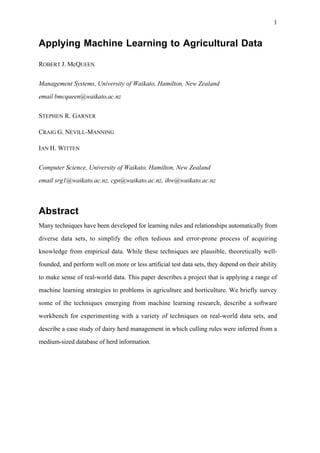
14. 14
• health problems;
• history of difficult calving;
• undesirable temperament traits (kicking, jumping fences);
• not being in calf for the following season.
The Livestock Improvement Corporation hoped that the machine learning project
investigation of their data might provide insight into the rules that farmers actually use to
make their culling decisions, enabling the corporation to provide better information to farmers
in the future. They provided data from ten herds, over six years, representing 19 000
records, each containing 705 attributes. These attributes are summarized in Table 3.
INITIAL DATA STRUCTURING
The machine learning tools used for the analysis were primarily C4.5 (Quinlan, 1992) and
FOIL (Quinlan, 1990). The initial raw data set as received from the Livestock Improvement
Corporation was run through C4.5 on the workbench. Classification was done on the fate
code attribute, which can take the values sold, dead, lost and unknown. The resulting tree,
shown in Figure 4, proved disappointing.
At the root of the tree is the transfer out date attribute. This implies that the culling
decision for a particular cow is based mainly on the date on which it is culled, rather than on
any attributes of the cow. Next, the date of birth is used, but as the culling decisions take
place in different years, an absolute date is not particularly meaningful. The cows age would
be useful, but is not explicitly present in the data set. The cause of fate attribute is strongly
associated with the fate code; it contains a coded explanation of the reason for culling. This
attribute is assigned a value after the culling decision is made, so it is not available to the
farmer when making the culling decision. Furthermore, we would like to be able to predict
this attribute—in particular the low production value—rather than include it in the tree as a
decision indicator. The presence of this attribute made the classification accuracy artificially
high, predicting the culling decision correctly 95% of the time on test data. Mating date is
another absolute date attribute, and animal key is simply a 7-digit identifier.
The problems with this decision tree stem from the denormalization of the database used

15. 15
to produce the input, and the representation of particular attributes. The solutions to these
problems are discussed below.
The effects of denormalization
Most machine learning techniques expect as input a set of tuples, analogous to one relation in
a database. Real databases, however, invariably contain more than one relation. The relational
operator join takes several relations and produces a single one from them, but this
denormalizes the database, introducing duplication and dependencies between attributes.
Dependencies in the data are quickly discovered by machine learning techniques, producing
trivial rules that relate two attributes. It is therefore necessary to modify the data or the scheme
to ignore these dependencies before interesting relationships can be discovered. In the project
described here, trivial relationships (such as between the fate code and cause of fate attributes)
are removed after inspecting decision trees by omitting one of the attributes from
consideration.
In this particular data set, a more serious problem stemmed from the joining of data from
several seasons. Each cow has particular attributes that remain constant throughout its
lifetime, for example animal key and date of birth. Other data, such as the number of weeks
of lactation, are recorded on a seasonal basis. In addition to this, monthly tests generate
production data, and movements from herd to herd are recorded at various times as they
occur. This means that data from several different years, months, and transfers were included
in the original record which was nominally for one year; data that should ideally be
considered separately (see Table 3).
Although culling decisions can occur at any point in the lactation season, the basic
decision to retain or remove an animal from the herd may be considered, for the purposes of
this investigation, to be made on an annual basis. Annual records should contain only
information about that year, and perhaps previous years, but not “foresight” information on
subsequent data or events as may have been included through the original extract from the
database. The dataset was renormalized into yearly records, taking care that “foresight”
information was excluded. Where no movement information (which included culling

16. 16
information) was recorded for a particular year, a retain decision replaces the missing value.
Monthly information was replaced by a yearly summary. While the data set was not fully
normalized (dependencies between animal key and date of birth still existed, for example), it
was normalized sufficiently for this particular application.
Attribute representation
The absolute dates included in the original data are not particularly useful. Once the database
is normalized into yearly records, these dates can be expressed relative to the year that the
record represents. In general, the accuracy of these dates need only be to the nearest year,
reducing the partitioning process evident in Figure 4.
In a discussion with staff from the Livestock Improvement Corporation, it was suggested
that a culling decision may not be based on a cow’s absolute performance, but on its
performance relative to the rest of the herd. To test this hypothesis, attributes were added to
the database representing the difference in production from the average production over the
cow’s herd. In order to prevent overly biasing the learning process, all the original attributes
were retained in the data set, and derived attributes added to the records were not
distinguished in any way. It was left to the machine learning schemes to decide if they were
more helpful for classification than the original attributes. Throughout this process, meetings
were held with staff at the Livestock Improvement Corporation. Discussions would often
result in the proposal of more derived attributes, and the clarification of the meaning of
particular attributes. Staff were also able to evaluate the plausibility of rules, which was
helpful in the early stages when recreating existing knowledge was a useful measure of the
correctness of our approach.
An obvious step would be to automate the production of derived attributes, to speed up
preprocessing and avoid human bias. However, the space of candidates is extremely large,
given the number of operations that can be performed on pairs of attributes. Typing the
attributes, and defining the operations which are meaningful on each type, would reduce the
space of possible derived attributes. For example, if the absolute dates in the original data are
defined as dates, and subtraction defined to be the only useful operator on dates, then the

17. 17
number of derived attributes would be considerably reduced, and useful attributes such as age
would still be produced. This is an interesting and challenging problem for investigation in
the future.
SUBSEQUENT C4.5 RUNS WITH MODIFIED DATA
After normalizing the data and adding derived attributes, C4.5 produced the tree in Figure 5.
Here, the fate code, cause of fate and transfer out date attributes have been transformed into a
status code which can take the values culled or retained. For a particular year, if a cow has
already been culled in a past season, or if it has not yet been born, the record is removed. If
the cow is alive in the given year, and is not transferred in that year, then it is marked as
retained. If it is transferred in that year, then it is marked culled. If, however, it died of
disease or some other factor outside the farmer’s control, the record is removed. After all, the
aim of this exercise is to discover the farmer’s culling rules rather than the incidence of
disease and injury.
The tree in Figure 5 is much more compact than the full tree shown in Figure 4. It was
produced with 30% of the instances, and correctly classifies 95% of the remaining instances.
The unconditional retention of cows two years or younger is due to the fact that they have not
begun lactation, and no measurements of their productive potential have yet been made. The
next decision is based on the cow’s worth as a breeding animal, which is calculated from the
earnings of the cow’s offspring. The volume of milk that the cow produces is used for the
final decision. The decisions in this tree are plausible from a farming perspective, and the
compactness and correctness of the tree indicate that it is a good explanation of the culling
decision. It is interesting to note that the tree consists entirely of derived attributes, further
emphasizing the importance of the preprocessing step.
Conclusions and future directions
From the work completed on the Livestock Improvement Corporation data it was possible
to isolate three steps that are necessary for the extraction of rules from a database.
The first step is extracting the data from its original form (in this case relational) to a two-

18. 18
dimensional flat-file form suitable for processing by the machine learning programs in the
workbench. This step is basically mechanical, and in principle could be achieved by simple
join operations on the database tables. In practice, however, the quality of the data—in
particular the large number of missing values—makes this non-trivial. This step also involved
the creation of the transformed attributes (e.g. age instead of birth date) and combined
attributes (e.g. not left herd and positive milk test = retained in herd).
The second step involves gaining insight about the problem domain from the extracted
and transformed dataset. It was helpful during this step to try initial runs of the dataset
through the machine learning tools. Some of these runs identified attributes, such as cow
identification number, which clearly have nothing to do with the culling decision. Through
questions directed at the domain experts, a greater understanding of the meaning of these
attributes was obtained, resulting in a better selection of the attributes to be used.
The third step was the use of machine learning tools to generate rules. Once a reasonably
well-structured dataset had been prepared in the standard file format, it was an easy matter to
process the dataset through the different algorithms available in the WEKA workbench, and
compare the resulting rule sets. The rules which resulted were referred to domain experts, and
the feedback used to iterate through all three steps to obtain new results.
In each of these three steps, domain expertise was essential to complement the data
transformation and machine learning processing skills required to prepare and process the
data sets.
Is there a likely future scenario of an automatic and unattended machine learning algorithm
being turned loose for background overnight processing against large relational databases?
We think the potential for this kind of intelligent agent may be there, but that there is much
that has to be done in the interim to create new algorithms and processing techniques that can
discover meaning in large and complex relational data structures, rather than the small and
simple two-dimensional attribute tables that have been used in the tests of machine learning
that are reported in the literature.
In the shorter term, there may be a high payback in making machine learning techniques

19. 19
easily usable by domain experts, who have intimate understanding of the nature of their data
and its relationships. Current developments include an attribute editor to simplify the process
of deriving new attributes from the data. This interactive tool will provide functions to
compute new attributes based on combinations of attributes, as well as inter-record
calculations such as rates of change in time-series data.
Overall, WEKA is fulfilling its role of bringing the potential of machine learning from the
computer science laboratory into the hands of experts in diverse domains.
Acknowledgements
This work is supported by the New Zealand Foundation for Research, Science and
Technology. We gratefully acknowledge the helpful cooperation of the Livestock
Improvement Centre, the work of Rhys Dewar and Donna Neal, and the stimulating research
environment provided by the Waikato machine learning group.
References
Angluin, D. and Smith, C.H., 1983. Inductive inference: theory and methods. Computing
Surveys, 15: 237–269.
Bareiss, A.R. Porter, B.W. and Weir, C.C. 1988, PROTOS: an exemplar-based learning
apprentice. Int. J. Man Machine Studies. 29(5), 549-561
Breiman, L., and Friedman, J.H., Olshen, R., and Stone C., 1984. Classification and
regression trees. Wadsworth International Group; Belmont, California.
Cameron-Jones, R.M., and Quinlan, J.R., 1993. Avoiding Pitfalls When Learning Recursive
Theories Proc. IJCAI 93, Morgan Kaufmann: 1050-1055
Cendrowska, J., 1987. PRISM: an algorithm for inducing modular rules. Int J Man-Machine
Studies, 27: 349–370.
Cheeseman, P., Kelly, J., Self, M., Stutz, J., Taylor, W., and Freeman, D., 1988.
AUTOCLASS: A Bayesian classification system. In: Laird, J. (Editor), Proc. of the Fifth
International Conference on Machine Learning. Ann Arbor, MI: Morgan Kaufmann: 54-

20. 20
64
DeJong, G. and Mooney, R. 1986. Explanation-based learning: an alternative view. Machine
Learning 1(2): 145-176
Fisher, D., 1987. Knowledge Acquisition Via Incremental Conceptual Clustering. Machine
Learning, 2: 139–172.
Gaines, B.R., 1991. The trade-off between knowledge and data in knowledge acquisition. In
Piatetsky–Shapiro and Frawley, 1991: 491–505.
Gennari, J.H., 1989. A survey of clustering methods., Technical Report 89-38, Irvine:
University of California, Dept. of Information and Computer Science.
Haussler, D., 1987. Learning conjunctive concepts in structural domains. Proc. AAAI: 466–
470.
Kaufman, K.A., and Michalski, R.S., 1993. EMERALD 2: An Integrated System of
Machine Learning and Discovery Programs to Support Education and Experimental
Research. Technical Report MLI 93-10, George Mason University.
Kodratoff, Y., Sleeman, D., Uszynski, M., Causse, K., and Craw, S., 1992. Building a
Machine Learning Toolbox. In: Steels, L. and Lepape, B. (Editors), Enhancing the
Knowledge Engineering Process, Elsevier Science Publishers B.V.: 81-108.
Kohavi, R., George, J., Long, R., Manley, D., and Pfleger, K., 1994. MLC++: A Machine
Learning Library in C++. Technical Report, Computer Science Department, Stanford
University.
Lebowitz, M. 1986. Concept learning in a rich input domain: Generalization-Based Memory.
In: R.S. Michalski, J.G. Carbonell and T.M. Mitchell (Editors), Machine Learning: An
Artificial Intelligence Approach, Volume II, Morgan Kaufmann, Los Altos, CA. 193-
214.
MacDonald, B.A. and Witten, I.H. 1989, A framework for knowledge acquisition through
techniques of concept learning. IEEE Trans Systems, Man and Cybernetics 19(3), 499-
512.

21. 21
Michalski, R.S. “Pattern recognition as rule-guided inductive inference.” 1980, IEEE
Transactions on Pattern Analysis and Machine Intelligence 2(4), 349-361.
Michalski, R.S. and Chilausky, R.L., 1980. Learning by being told and learning from
examples: an experimental comparison of the two methods of knowledge acquisition in
the context of developing an expert system for soybean disease diagnosis. International J
Policy Analysis and Information Systems, 4: 125–161
Michalski, R.S., 1983. A theory and methodology of inductive learning. Artificial
Intelligence, 20: 111–161.
Michalski, R.S., Davis, J.H., Bisht, V.S. and Sinclair, J.B., 1982. PLANT/ds: an expert
consulting system for the diagnosis of soybean diseases. Proc. European Conference on
Artificial Intelligence, Orsay, France, July: 133–138.
Mitchell, T.M., Keller, R.M. and Kedar-Cabelli, S.T., 1986. Explanation-based
generalization: a unifying view. Machine Learning 1(1) 47-80
Monk, T.J., Mitchell, S., Smith, L.A. and Holmes, G., 1994. Geometric comparison of
classifications and rule sets, Proc. AAAI workshop on knowledge discovery in
databases, Seattle, Washington, July: 395-406.
Mooney, R.J., 1992. Encouraging Experimental Results on Learning CNF. Technical
Report, University of Texas.
Murthy, S.K., Kasif, S., Salzberg, S., and Beigel, R., 1993. OC1: Randomized Induction
of Decision Trees. Proc. of the Eleventh National Conference on Artificial Intelligence.
Washington, D.C.: 322–327
Ousterhout, J. K., 1994. TCL and TK toolkit, Addison-Wesley.
Pazzani, M. and Kibler, D. 1992, The utility of knowledge in inductive learning. Machine
Learning 9(1), 57-94
Piatetsky–Shapiro, G. and Frawley, W.J. (Editors), 1991: Knowledge discovery in
databases. AAAI Press, Menlo Park, CA. 525 pp.

22. 22
Quinlan, J.R., 1986. Induction of decision trees. Machine Learning, 1: 81–106.
Quinlan, J.R., 1990. Learning Logical Definitions from Relations. Machine Learning, 5:
239-266.
Quinlan, J.R., 1991. Determinate Literals in Inductive Logic Programming. Proc. 12th
International Joint Conference on Artificial Intelligence: 746-750, Morgan Kaufmann.
Quinlan, J.R., 1992. C4.5: Programs for Machine Learning. Morgan Kaufmann. 302 pp.
Quinlan, J.R., and Cameron-Jones, R.M., 1993. FOIL: a midterm report. Proc. European
Conference on Machine Learning, Springer Verlag: 3-20
Schank, R.C., Collins, G.C. and Hunter, L.E., 1986. Transcending inductive category
formation in learning. Behavioral and Brain Sciences, 9: 639–651.
Winston, P.H. 1972. Learning structural descriptions from examples. in P.H. Winston, Ed.,
The Psychology of Computer Vision, McGraw-Hill, New York, 689-702.
Witten, I.H. and MacDonald, B.A. 1988 Using concept learning for knowledge acquisition,
Int. J. Man Machine Studies. 29(2) 171-196

23. 23
color: Tree-structured attribute shape:
regular-polygon oval
Linear attribute
size: 1
2
3
4
5
(a)
Attribute vector Vector of generalized attributes
(sample concept)
color and color and
size = and and
shape = shape = convex
(b) (c)
Figure 1 Attribute domain (adapted from Haussler, 1987)

24. 24
Environmental descriptors Condition of leaves Condition of stem
time of occurrence July leaf spots stem lodging
precipitation above normal leaf spot colour stem cankers
temperature normal colour of spot on other side canker lesion colour
cropping history 4 years yellow leaf spot halos reddish canker margin
damaged area whole fields leaf spot margins fruiting bodies on stem
severity mild raised leaf spots external decay of stem
plant height normal leaf spot growth mycelium on stem
leaf spot size external discolouration
Condition of seed normal shot-holing location of discolouration
mould growth absent shredding internal discolouration
discolouration absent leaf malformation sclerotia
discolouration colour — premature defoliation
size normal leaf mildew growth Condition of roots
shriveling absent leaf discolouration root rot
position of affected leaves root galls or cysts
Condition of fruit pods normal condition of lower leaves root sclerotia
fruit pods normal leaf withering and wilting
fruit spots absent
(a) Diagnosis Brown spot
(b) Rhizoctonia root rot IF [leaves=normal AND stem=abnormal AND
stem-cankers=below-soil-line AND canker-lesion-colour=brown]
OR [leaf-malformation=absent AND stem=abnormal AND
stem-cankers=below-soil-line AND canker-lesion-colour=brown]
Figure 2 Example record and rule in the soybean disease classification problem

25. 25
Figure 3 The WEKA user interface

26. 26
Transfer out date
<= 900420 > 900420
Transfer out date •••
<= 880217 > 880217
Unknown Animal Date of Birth
<= 860811 > 860811
Transfer out date Died
<= 890613 > 890613
Cause of fate •••
Injury Bloat Calving Grass Injury Low Other Milk Empty Old Udder
Trouble Staggers Producer Causes Fever age breakdown
Sold Died Sold Sold Sold Sold Sold Sold Sold Sold
Mating date
<= 890613 > 890613
Sold Animal Key
<= 2811510 > 2811510
Died Sold
Figure 4: Decision tree induced from raw herd data

27. 27
Age
<= 2 >2
Retained Payment BI
relative to herd
<= -10.8 > -10.8
Milk Volume PI Retained
relative to herd
<= -33.93 > -33.93
Culled Retained
Figure 5. Decision tree from processed data set

28. 28
1 Minimal rules A complete, correct, and minimal set of decision rules
2 Adequate rules A complete and correct set of rules that nevertheless contains
redundant rules and references to irrelevant attributes
3 Critical cases A critical set of cases described in terms of a minimal set of
relevant attributes with correct decisions
4 Source of cases A source of cases that contains such critical examples described in
terms of a minimal set of relevant attributes with correct decisions
5 Irrelevant attributes As for 4 but with cases described in terms of attributes which
include ones that are irrelevant to the decision
6 Incorrect decisions As for 4 but with only a greater-than-chance probability of correct
decisions
7 Irrelevant attributes As for 5 but with only a greater-than-chance probability of correct
and incorrect decisions decisions
Table 1 Levels of quality of input (Gaines, 1991)

29. 29
Scheme Learning approach Reference
Unsupervised AUTOCLASS Bayesian clustering Cheeseman et al. (1988)
CLASSWEB Incremental conceptual clustering Fisher et al. (1987), Fisher (1989)
Gennari (1989)
Supervised C4.5 Decision tree induction Quinlan (1992)
OC1 Oblique decision tree induction for Murthy et al. (1993)
numeric data
CNF & DNF Conjunctive and disjunctive normal Mooney (1992)
form decision trees respectively
PRISM DNF rule generator Cendrowska (1987)
INDUCT Improved PRISM Gaines (1991)
FOIL First-order inductive learner Quinlan (1990), Quinlan (1991),
Quinlan et al. (1993), Cameron-
Jones et al. (1993)
Table 2 Machine learning schemes currently included in the WEKA workbench

30. 30
Relation Number of Recording basis
attributes
Animal Birth Identification 3 Once
Animal Sire 1 Once
Animal 6 Once
Test Number Identification 1 Monthly
Animal Location 3×6 When moved
Female Parturition 5 When calving
New Born Animal 3×4 When calving
Female Reproductive Status 3 Once
Female mating 10 × 3 When mated
Animal Lactation 60 Yearly
Test Day Production Detail 12 × 43 Monthly
Non production trait survey 30 Once
Animal Cross Breed 3×2 Once
Animal Lactation—Dam 12 Once
Female Parturition—Dam 5 Once
New Born Animal—Dam 3×4 When dam calves
Animal—Dam—Sire 2 Once
Table 3: Dairy herd database relations