Distributional semantic models

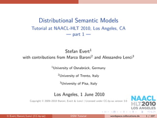
Distributional Semantic Models
Tutorial at NAACL-HLT 2010, Los Angeles, CA
— part 1 —

Stefan Evert1
with contributions from Marco Baroni2 and Alessandro Lenci3

1 University of Osnabrück, Germany
2 University of Trento, Italy
3 University of Pisa, Italy

Los Angeles, 1 June 2010
Copyright © 2009–2010 Baroni, Evert & Lenci | Licensed under CC-by-sa version 3.0

© Evert/Baroni/Lenci (CC-by-sa) DSM Tutorial wordspace.collocations.de 1 / 107

Outline

Outline

Introduction
The distributional hypothesis
General overview
Three famous DSM examples

Taxonomy of DSM parameters
Deﬁnition & overview
DSM parameters
Examples

Usage and evaluation of DSM
What to do with DSM distances
Evaluation: semantic similarity and relatedness
Attributional similarity
Relational similarity


Introduction The distributional hypothesis

Outline

Introduction
General overview

DSM parameters
Examples




Meaning & distribution

“Die Bedeutung eines Wortes liegt in seinem Gebrauch.”
— Ludwig Wittgenstein





“You shall know a word by the company it keeps!”
— J. R. Firth (1957)





“You shall know a word by the company it keeps!”
— J. R. Firth (1957)

Distributional hypothesis (Zellig Harris 1954)



What is the meaning of “bardiwac”?




He handed her her glass of bardiwac.




Beef dishes are made to complement the bardiwacs.




Nigel staggered to his feet, face ﬂushed from too much
bardiwac.




bardiwac.
Malbec, one of the lesser-known bardiwac grapes, responds
well to Australia’s sunshine.




bardiwac.
I dined oﬀ bread and cheese and this excellent bardiwac.




bardiwac.
The drinks were delicious: blood-red bardiwac as well as light,
sweet Rhenish.


bardiwac is a heavy red alcoholic beverage made from grapes



Real-life concordance & word sketch
http://beta.sketchengine.co.uk/



A thought experiment: deciphering hieroglyphs

get sij ius hir iit kil

(knife) naif 51 20 84 0 3 0
(cat) ket 52 58 4 4 6 26
??? dog 115 83 10 42 33 17
(boat) beut 59 39 23 4 0 0
(cup) kap 98 14 6 2 1 0
(pig) pigij 12 17 3 2 9 27
(banana) nana 11 2 2 0 18 0





(knife) naif 51 20 84 0 3 0
(cat) ket 52 58 4 4 6 26
??? dog 115 83 10 42 33 17
(boat) beut 59 39 23 4 0 0
(cup) kap 98 14 6 2 1 0
(pig) pigij 12 17 3 2 9 27
(banana) nana 11 2 2 0 18 0

sim(dog, naif ) = 0.770





(knife) naif 51 20 84 0 3 0
(cat) ket 52 58 4 4 6 26
??? dog 115 83 10 42 33 17
(boat) beut 59 39 23 4 0 0
(cup) kap 98 14 6 2 1 0
(pig) pigij 12 17 3 2 9 27
(banana) nana 11 2 2 0 18 0

sim(dog, pigij ) = 0.939





(knife) naif 51 20 84 0 3 0
(cat) ket 52 58 4 4 6 26
??? dog 115 83 10 42 33 17
(boat) beut 59 39 23 4 0 0
(cup) kap 98 14 6 2 1 0
(pig) pigij 12 17 3 2 9 27
(banana) nana 11 2 2 0 18 0

sim(dog, ket ) = 0.961



English as seen by the computer . . .

get see use hear eat kill

knife naif 51 20 84 0 3 0
cat ket 52 58 4 4 6 26
dog dog 115 83 10 42 33 17
boat beut 59 39 23 4 0 0
cup kap 98 14 6 2 1 0
pig pigij 12 17 3 2 9 27
banana nana 11 2 2 0 18 0

verb-object counts from British National Corpus



Geometric interpretation

row vector xdog
describes usage of
word dog in the get see use hear eat kill
corpus knife 51 20 84 0 3 0
cat 52 58 4 4 6 26
can be seen as
dog 115 83 10 42 33 17
coordinates of point boat 59 39 23 4 0 0
in n-dimensional cup 98 14 6 2 1 0
Euclidean space pig 12 17 3 2 9 27
banana 11 2 2 0 18 0

co-occurrence matrix M



Two dimensions of English V−Obj DSM
row vector xdog

120
describes usage of
word dog in the

100
corpus
knife
can be seen as q

80
coordinates of point
in n-dimensional use

60
Euclidean space
illustrated for two
40

dimensions: boat
q
get and use
20

dog
cat q
xdog = (115, 10) q
0

0 20 40 60 80 100 120

get



similarity = spatial

120
proximity
(Euclidean dist.)

100
location depends on knife
frequency of noun q

80
(fdog ≈ 2.7 · fcat )
use

60
40

boat
q d=5
7.5
20

dog
cat d = 63.3 q
q
0

0 20 40 60 80 100 120

get




120
proximity
(Euclidean dist.)

100
frequency of noun q

80
(fdog ≈ 2.7 · fcat )
use
direction more
important than 60
40

location
boat
q
20

dog
cat q
q
0

0 20 40 60 80 100 120

get




120
proximity
(Euclidean dist.)

100
frequency of noun q

80
(fdog ≈ 2.7 · fcat ) q
use
direction more
important than 60
40

location
boat q
normalise “length” q
20

xdog of vector dog
cat q
q
q
0

0 20 40 60 80 100 120

get




120
proximity
(Euclidean dist.)

100
frequency of noun q

80
(fdog ≈ 2.7 · fcat ) q
use
direction more
60
α = 54.3°
important than 40

location
boat q
normalise “length” q
20

xdog of vector dog
cat q
q
or use angle α as q
0

distance measure 0 20 40 60 80 100 120

get



Semantic distances
Word space clustering of concrete nouns (V−Obj from BNC)

main result of distributional

1.2
1.0
analysis are “semantic”

0.8
distances between words

0.6
Cluster size

0.4
typical applications

0.2
nearest neighbours

0.0
qqqqqqqqqqqqqqqqqqqqqqqqqqqqqqqqqqqqqqqqqqqq

potato
onion
cat
banana
chicken
mushroom
corn
dog
pear
cherry
lettuce
penguin
swan
eagle
owl
duck
elephant
pig
cow
lion
helicopter
peacock
turtle
car
pineapple
boat
rocket
truck
motorcycle
snail
ship
chisel
scissors
screwdriver
pencil
hammer
telephone
knife
spoon
pen
kettle
bottle
cup
bowl
clustering of related words
construct semantic map
Semantic map (V−Obj from BNC)

0.6
potato kettle
onion q q bird
q q
q groundAnimal
mushroom q fruitTree

0.4
q chicken q green
q cup
q q tool
q banana q vehicle
cat bowl
q lettuce q bottle

0.2
q q pen
cherry q q q
corn
dog q q pear
pig lion
q pineapple
q
q
spoon
0.0

q ship q
cow car q
q boat q
elephant telephone q q knife
snail
qq pencil
eagle duck q
rocket q
q
−0.2

q
q owl
swan qq motorcycle hammer
q peacock truck q
q q
penguin
q
q helicopter chisel
−0.4

turtle q q screwdriver
q
scissors

−0.4 −0.2 0.0 0.2 0.4 0.6 0.8


Introduction General overview

Outline

Introduction
General overview

DSM parameters
Examples




Tutorial overview

1. Introduction & examples
2. Taxonomy of DSM parameters
3. Usage and evaluation of DSM spaces
4. Elements of matrix algebra
5. Making sense of DSM
6. Current research topics & future directions

Realistically, we’ll get through parts 1–3 today. But you can ﬁnd out about
matrix algebra and the other advanced topics in the handouts available from
the course Web site.



Further information

Handouts & other materials vailable from homepage at
http://wordspace.collocations.de/

will be extended during the next few months
Tutorial is open source (CC), and can be downloaded from
http://r-forge.r-project.org/projects/wordspace/
Compact DSM textbook in preparation for Synthesis Lectures
on Human Language Technologies (Morgan & Claypool)

This tutorial is based on joint work with
Marco Baroni and Alessandro Lenci



A very brief history of DSM

Introduced to computational linguistics in early 1990s
following the probabilistic revolution (Schütze 1992, 1998)
Other early work in psychology (Landauer and Dumais 1997;
Lund and Burgess 1996)

inﬂuenced by Latent Semantic Indexing (Dumais et al. 1988)
and eﬃcient software implementations (Berry 1992)


Renewed interest in recent years
2007: CoSMo Workshop (at Context ’07)


2008: ESSLLI Lexical Semantics Workshop & Shared Task,
Special Issue of the Italian Journal of Linguistics


2009: GeMS Workshop (EACL 2009), DiSCo Workshop
(CogSci 2009), ESSLLI Advanced Course on DSM


2009: GeMS Workshop (EACL 2009), DiSCo Workshop
(CogSci 2009), ESSLLI Advanced Course on DSM
2010: 2nd GeMS Workshop (ACL 2010), ESSLLI Workhsop on
Compositionality & DSM, Special Issue of JNLE (in prep.),
Computational Neurolinguistics Workshop (NAACL-HLT 2010
— don’t miss it this Sunday!)



Some applications in computational linguistics

Unsupervised part-of-speech induction (Schütze 1995)
Word sense disambiguation (Schütze 1998)
Query expansion in information retrieval (Grefenstette 1994)
Synonym tasks & other language tests
(Landauer and Dumais 1997; Turney et al. 2003)
Thesaurus compilation (Lin 1998a; Rapp 2004)
Ontology & wordnet expansion (Pantel et al. 2009)
Attachment disambiguation (Pantel 2000)
Probabilistic language models (Bengio et al. 2003)
Subsymbolic input representation for neural networks
Many other tasks in computational semantics:
entailment detection, noun compound interpretation,
identiﬁcation of noncompositional expressions, . . .


Introduction Three famous DSM examples

Outline

Introduction
General overview

DSM parameters
Examples




Latent Semantic Analysis (Landauer and Dumais 1997)
Corpus: 30,473 articles from Grolier’s Academic American
Encyclopedia (4.6 million words in total)

articles were limited to ﬁrst 2,000 characters
Word-article frequency matrix for 60,768 words
row vector shows frequency of word in each article
Logarithmic frequencies scaled by word entropy
Reduced to 300 dim. by singular value decomposition (SVD)
borrowed from LSI (Dumais et al. 1988)

central claim: SVD reveals latent semantic features,
not just a data reduction technique
Evaluated on TOEFL synonym test (80 items)
LSA model achieved 64.4% correct answers
also simulation of learning rate based on TOEFL results



Word Space (Schütze 1992, 1993, 1998)

Corpus: ≈ 60 million words of news messages (New York
Times News Service)
Word-word co-occurrence matrix
20,000 target words & 2,000 context words as features
row vector records how often each context word occurs close
to the target word (co-occurrence)
co-occurrence window: left/right 50 words (Schütze 1998)
or ≈ 1000 characters (Schütze 1992)
Rows weighted by inverse document frequency (tf.idf)
Context vector = centroid of word vectors (bag-of-words)

goal: determine “meaning” of a context
Reduced to 100 SVD dimensions (mainly for eﬃciency)
Evaluated on unsupervised word sense induction by clustering
of context vectors (for an ambiguous word)
induced word senses improve information retrieval performance


HAL (Lund and Burgess 1996)

HAL = Hyperspace Analogue to Language
Corpus: 160 million words from newsgroup postings
Word-word co-occurrence matrix
same 70,000 words used as targets and features
co-occurrence window of 1 – 10 words
Separate counts for left and right co-occurrence
i.e. the context is structured
In later work, co-occurrences are weighted by (inverse)
distance (Li et al. 2000)
Applications include construction of semantic vocabulary
maps by multidimensional scaling to 2 dimensions



Many parameters . . .

Enormous range of DSM parameters and applications
Examples showed three entirely diﬀerent models, each tuned
to its particular application
¯ Need overview of DSM parameters & understand their eﬀects


Taxonomy of DSM parameters Deﬁnition & overview

Outline

Introduction
General overview

DSM parameters
Examples




General deﬁnition of DSMs

A distributional semantic model (DSM) is a scaled and/or
transformed co-occurrence matrix M, such that each row x
represents the distribution of a target term across contexts.

get see use hear eat kill
knife 0.027 -0.024 0.206 -0.022 -0.044 -0.042
cat 0.031 0.143 -0.243 -0.015 -0.009 0.131
dog -0.026 0.021 -0.212 0.064 0.013 0.014
boat -0.022 0.009 -0.044 -0.040 -0.074 -0.042
cup -0.014 -0.173 -0.249 -0.099 -0.119 -0.042
pig -0.069 0.094 -0.158 0.000 0.094 0.265
banana 0.047 -0.139 -0.104 -0.022 0.267 -0.042

Term = word, lemma, phrase, morpheme, . . .



General deﬁnition of DSMs

Mathematical notation:
m × n co-occurrence matrix M (example: 7 × 6 matrix)
m rows = target terms
n columns = features or dimensions
 
x11 x12 · · · x1n
 x21 x22 · · · x2n 
M= .
 
. . 
 .. .
. . 
.
xm1 xm2 · · · xmn
distribution vector xi = i-th row of M, e.g. x3 = xdog
components xi = (xi1 , xi2 , . . . , xin ) = features of i-th term:

x3 = (−0.026, 0.021, −0.212, 0.064, 0.013, 0.014)
= (x31 , x32 , x33 , x34 , x35 , x36 )



Overview of DSM parameters

Linguistic pre-processing (deﬁnition of terms)




⇓
Term-context vs. term-term matrix




⇓
⇓
Size & type of context / structured vs. unstructered




⇓
⇓
⇓
Geometric vs. probabilistic interpretation




⇓
⇓
⇓
⇓
Feature scaling




⇓
⇓
⇓
⇓
Feature scaling
⇓
Normalisation of rows and/or columns




⇓
⇓
⇓
⇓
Feature scaling
⇓
⇓
Similarity / distance measure




⇓
⇓
⇓
⇓
Feature scaling
⇓
⇓
⇓
Compression


Taxonomy of DSM parameters DSM parameters

Outline

Introduction
General overview

DSM parameters
Examples




Corpus pre-processing

Minimally, corpus must be tokenised § identify terms
Linguistic annotation
part-of-speech tagging
lemmatisation / stemming
word sense disambiguation (rare)
shallow syntactic patterns
dependency parsing




dependency parsing
Generalisation of terms
often lemmatised to reduce data sparseness:
go, goes, went, gone, going § go
POS disambiguation (light/N vs. light/A vs. light/V)
word sense disambiguation (bankriver vs. bankﬁnance )




dependency parsing
Generalisation of terms
often lemmatised to reduce data sparseness:
go, goes, went, gone, going § go
POS disambiguation (light/N vs. light/A vs. light/V)
word sense disambiguation (bankriver vs. bankfinance )
Trade-off between deeper linguistic analysis and
need for language-specific resources
possible errors introduced at each stage of the analysis
even more parameters to optimise / cognitive plausibility


Eﬀects of pre-processing
Nearest neighbours of walk (BNC)

word forms lemmatised corpus
stroll hurry
walking stroll
walked stride
go trudge
path amble
drive wander
ride walk-nn
wander walking
sprinted retrace
sauntered scuttle



Eﬀects of pre-processing
Nearest neighbours of arrivare (Repubblica)

word forms lemmatised corpus
giungere giungere
raggiungere aspettare
arrivi attendere
raggiungimento arrivo-nn
raggiunto ricevere
trovare accontentare
raggiunge approdare
arrivasse pervenire
arriverà venire
concludere piombare




⇓
⇓
⇓
⇓
Feature scaling
⇓
⇓
⇓
Compression




Term-context matrix records frequency of term in each individual
context (typically a sentence or document)

doc1 doc2 doc3 ···
boat 1 3 0 ···
cat 0 0 2 ···
dog 1 0 1 ···

Typical contexts are non-overlapping textual units (Web page,
encyclopaedia article, paragraph, sentence, . . . )




Term-context matrix records frequency of term in each individual
context (typically a sentence or document)

doc1 doc2 doc3 ···
boat 1 3 0 ···
cat 0 0 2 ···
dog 1 0 1 ···

Typical contexts are non-overlapping textual units (Web page,
encyclopaedia article, paragraph, sentence, . . . )
Contexts can also be generalised, e.g.
bag of content words
speciﬁc pattern of POS tags
subcategorisation pattern of target verb
Term-context matrix is usually very sparse




Term-term matrix records co-occurrence frequencies of context
terms for each target term (often target terms = context terms)

see use hear ···
boat 39 23 4 ···
cat 58 4 4 ···
dog 83 10 42 ···




Term-term matrix records co-occurrence frequencies of context
terms for each target term (often target terms = context terms)

see use hear ···
boat 39 23 4 ···
cat 58 4 4 ···
dog 83 10 42 ···

Diﬀerent types of contexts (Evert 2008)
surface context (word or character window)
textual context (non-overlapping segments)
syntactic contxt (speciﬁc syntagmatic relation)
Can be seen as smoothing of term-context matrix
average over similar contexts (with same context terms)
data sparseness reduced, except for small windows




⇓
⇓
⇓
⇓
Feature scaling
⇓
⇓
⇓
Compression



Surface context

Context term occurs within a window of k words around target.

The silhouette of the sun beyond a wide-open bay on the lake; the
sun still glitters although evening has arrived in Kuhmo. It’s
midsummer; the living room has its instruments and other objects
in each of its corners.

Parameters:
window size (in words or characters)
symmetric vs. one-sided window
uniform or “triangular” (distance-based) weighting
window clamped to sentences or other textual units?



Eﬀect of diﬀerent window sizes
Nearest neighbours of dog (BNC)

2-word window 30-word window
cat kennel
horse puppy
fox pet
pet bitch
rabbit terrier
pig rottweiler
animal canine
mongrel cat
sheep to bark
pigeon Alsatian



Textual context

Context term is in the same linguistic unit as target.


Parameters:
type of linguistic unit
sentence
paragraph
turn in a conversation
Web page



Syntactic context

Context term is linked to target by a syntactic dependency
(e.g. subject, modiﬁer, . . . ).


Parameters:
types of syntactic dependency (Padó and Lapata 2007)
direct vs. indirect dependency paths
direct dependencies
direct + indirect dependencies
homogeneous data (e.g. only verb-object) vs.
heterogeneous data (e.g. all children and parents of the verb)
maximal length of dependency path


“Knowledge pattern” context

Context term is linked to target by a lexico-syntactic pattern
(text mining, cf. Hearst 1992, Pantel & Pennacchiotti 2008, etc.).

In Provence, Van Gogh painted with bright colors such as red and
yellow. These colors produce incredible effects on anybody looking
at his paintings.

Parameters:
inventory of lexical patterns
lots of research to identify semantically interesting patterns
(cf. Almuhareb & Poesio 2004, Veale & Hao 2008, etc.)
fixed vs. flexible patterns
patterns are mined from large corpora and automatically
generalised (optional elements, POS tags or semantic classes)



Structured vs. unstructured context

In unstructered models, context specification acts as a filter
determines whether context tokens counts as co-occurrence
e.g. linked by specific syntactic relation such as verb-object



Structured vs. unstructured context

In unstructered models, context specification acts as a filter
determines whether context tokens counts as co-occurrence
e.g. linked by specific syntactic relation such as verb-object

In structured models, context words are subtyped
depending on their position in the context
e.g. left vs. right context, type of syntactic relation, etc.



Structured vs. unstructured surface context

A dog bites a man. The man’s dog bites a dog. A dog bites a man.

unstructured bite
dog 4
man 3



Structured vs. unstructured surface context


unstructured bite
dog 4
man 3


structured bite-l bite-r
dog 3 1
man 1 2



Structured vs. unstructured dependency context


unstructured bite
dog 4
man 2



Structured vs. unstructured dependency context


unstructured bite
dog 4
man 2


structured bite-subj bite-obj
dog 3 1
man 0 2



Comparison
Unstructured context
data less sparse (e.g. man kills and kills man both map to the
kill dimension of the vector xman )

Structured context
more sensitive to semantic distinctions
(kill-subj and kill-obj are rather diﬀerent things!)
dependency relations provide a form of syntactic “typing” of
the DSM dimensions (the “subject” dimensions, the
“recipient” dimensions, etc.)
important to account for word-order and compositionality




⇓
⇓
⇓
⇓
Feature scaling
⇓
⇓
⇓
Compression



row vectors as points or arrows in n-dim. space
very intuitive, good for visualisation
use techniques from geometry and linear algebra




Probabilistic interpretation
co-occurrence matrix as observed sample statistic
“explained” by generative probabilistic model
recent work focuses on hierarchical Bayesian models
probabilistic LSA (Hoﬀmann 1999), Latent Semantic
Clustering (Rooth et al. 1999), Latent Dirichlet Allocation
(Blei et al. 2003), etc.
explicitly accounts for random variation of frequency counts
intuitive and plausible as topic model


focus exclusively on geometric interpretation in this tutorial




⇓
⇓
⇓
⇓
Feature scaling
⇓
⇓
⇓
Compression



Feature scaling

Feature scaling is used to “discount” less important features:
Logarithmic scaling: x = log(x + 1)
(cf. Weber-Fechner law for human perception)



Feature scaling

Relevance weighting, e.g. tf.idf (information retrieval)



Feature scaling

Relevance weighting, e.g. tf.idf (information retrieval)
Statistical association measures (Evert 2004, 2008) take
frequency of target word and context feature into account
the less frequent the target word and (more importantly) the
context feature are, the higher the weight given to their
observed co-occurrence count should be (because their
expected chance co-occurrence frequency is low)
diﬀerent measures – e.g., mutual information, log-likelihood
ratio – diﬀer in how they balance observed and expected
co-occurrence frequencies



Association measures: Mutual Information (MI)

word1 word2 fobs f1 f2
dog small 855 33,338 490,580
dog domesticated 29 33,338 918




dog small 855 33,338 490,580

Expected co-occurrence frequency:
f1 · f 2
fexp =
N




dog small 855 33,338 490,580

f1 · f 2
fexp =
N
Mutual Information compares observed vs. expected frequency:
fobs N · fobs
MI(w1 , w2 ) = log2 = log2
fexp f 1 · f2




dog small 855 33,338 490,580

f1 · f 2
fexp =
N
Mutual Information compares observed vs. expected frequency:
fobs N · fobs
MI(w1 , w2 ) = log2 = log2
fexp f 1 · f2

Disadvantage: MI overrates combinations of rare terms.



Other association measures

Log-likelihood ratio (Dunning 1993) has more complex form, but
its “core” is known as local MI (Evert 2004).

local-MI(w1 , w2 ) = fobs · MI(w1 , w2 )






word1 word2 fobs MI local-MI
dog small 855 3.96 3382.87
dog domesticated 29 6.85 198.76
dog sgjkj 1 10.31 10.31






word1 word2 fobs MI local-MI
dog small 855 3.96 3382.87
dog domesticated 29 6.85 198.76
dog sgjkj 1 10.31 10.31

The t-score measure (Church and Hanks 1990) is popular in
lexicography:
fobs − fexp
t-score(w1 , w2 ) = √
fobs
Details & many more measures: http://www.collocations.de/




⇓
⇓
⇓
⇓
Feature scaling
⇓
⇓
⇓
Compression



Normalisation of row vectors

geometric distances only

120
make sense if vectors are

100
normalised to unit length
knife
divide vector by its length: q

80
q

use
x/ x

60
40
normalisation depends on
boat q
distance measure! q

20
dog
q
special case: scale to cat
q
q
0

relative frequencies with 0 20 40 60 80 100 120

x 1 = |x1 | + · · · + |xn | get



Scaling of column vectors

In statistical analysis and machine learning, features are
usually centred and scaled so that

mean µ=0
variance σ2 = 1

In DSM research, this step is less common for columns of M
centring is a prerequisite for certain dimensionality reduction
and data analysis techniques (esp. PCA)
scaling may give too much weight to rare features



Scaling of column vectors

In statistical analysis and machine learning, features are
usually centred and scaled so that

mean µ=0
variance σ2 = 1

In DSM research, this step is less common for columns of M
centring is a prerequisite for certain dimensionality reduction
and data analysis techniques (esp. PCA)
scaling may give too much weight to rare features
M cannot be row-normalised and column-scaled at the same
time (result depends on ordering of the two steps)




⇓
⇓
⇓
⇓
Feature scaling
⇓
⇓
⇓
Compression



Geometric distance

Distance between vectors x2

u, v ∈ Rn § (dis)similarity 6
u
u = (u1 , . . . , un )
5
v = (v1 , . . . , vn ) d1 (u, v) = 5
4
d2 (u, v) = 3.6
3

v
2

1

x1
1 2 3 4 5 6



Geometric distance

Distance between vectors x2

u, v ∈ Rn § (dis)similarity 6
u
u = (u1 , . . . , un )
5
v = (v1 , . . . , vn ) d1 (u, v) = 5
4
Euclidean distance d2 (u, v) d2 (u, v) = 3.6
3

v
2

1

x1
1 2 3 4 5 6

d2 (u, v) := (u1 − v1 )2 + · · · + (un − vn )2


Distributional semantic models

Distributional semantic models

Empfohlen

Empfohlen

Weitere ähnliche Inhalte

Was ist angesagt?

Was ist angesagt? (10)

Kürzlich hochgeladen

Kürzlich hochgeladen (20)

Distributional semantic models