Rotordynamics Study

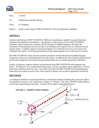
1. Technical Report BPC-DCA-03-046
Page 1 of 20
Date: 11/04/03
To: Al Robertson and Bob Thomas
From: D. Ansbigian
Subject: Analysis and Testing of MSC/NASTRAN’s New Rotordynamic Capability
ABSTRACT
Analysis and Testing of MSC/NASTRAN’s 2004 new rotordynamic capability was performed and
compared with theoretical calculations. The objective of this report is to have MSC/NASTRAN
determine critical frequencies, compare with the theoretical Campbell diagram, and check the
correlation of bearing loads and run-outs due to an imbalance for a typical rotor as a function of rotor
angular speed. A stability analysis is being put together for verification, however, not in time to be
included in this report. It will be performed and written under separate cover in the next few months.
The MSC/NASTRAN results showed excellent correlation with the theoretical Campbell diagram.
Comparison of the two is illustrated later on in this report. In addition, the critical speed calculations for
the forward cylindrical whirl and the forward conical whirl are in excellent agreement with theory.
Finally, a frequency response analysis was performed using MSC/NASTRAN and compared with
theory. The objective was to determine bearing loads, run-outs, and phase when subjected to a 50 inch-
gram static imbalance from the rotor. The results show that the MSC/NASTRAN calculated bearing
loads and zero-to-peak run-outs at the critical speed of interest were in perfect agreement with theory.
DISCUSSION
A verification problem was developed that has a closed-form solution including the gyroscopic effects.
The problem as stated is a 10” long hollow cylinder, 2” OD and 1” ID, with a 100 lb/in spring stiffness
at each end, representing the bearings. A sketch of the model is depicted in Figure 1.
21
FIGURE 1 - VERIFICATION MODEL RBE
11
Ksprings = 100 lb/in (for all)
2” OD
1” ID
1
RBE
10”

2. Technical Report BPC-DCA-03-046
Page 2 of 20
The model was developed using 20 CBAR elements. Material properties used in the model are shown
below in Table 1.
Table 1:
Material Properties
Item PATRAN Designation Description Steel
E (ksi) E1 Modulus of Elasticity 30.E6
NUxy NU12 Poisson’s Ratio in XY-plane 0.3
Density (lb/in3) ρ Density .2835
Using MSC/NASTRAN 2004, the rotor ends are attached to the support bearings via RBE2 elements.
Then from there, the bearings are represented by CELAS1 (spring) elements connected to ground. The
bearings were assigned a stiffness value of 100 lb/in. In addition, a stiffness of 100 lb/in was also
included in the model in the axial direction to represent the connection from the rotor to the stator. This
spring element simulates a magnet between the rotor and stator. The bulk data file used to run this case
is given in Enclosure (1).
MODAL ANALYSIS RESULTS
The model was exercised solution sequence (SOL) 107, which is a complex eigenvalue solution.
Complex eigenvalue analysis is necessary when the matrices contain unsymmetric terms, damping
effects, or complex numbers where real modes analysis cannot be used. It is typically used for the
analysis of rotating bodies such as this. The eigenvalue method chosen for this analysis was the
complex Hessenberg Method. The solution was run at 0, 10K, 30K, and 50KRPM and the real and
imaginary roots were determined without damping. Table 2 below lists the key modes of vibration
determined from the MSC/NASTRAN 2004 solution.
Table 2
MSC/NASTRAN 2004 RESULTS
Frequencies and Mode Shapes
Forward Backward
RPM Cylindrical Conical Cylindrical Conical
0 17.11 29.56 -17.11 -29.56
10,000 17.11 36.43 -17.11 -23.99
30,000 17.11 53.62 -17.11 -16.30
50,000 17.11 74.00 -17.11 -11.81
The cylindrical and conical whirl modes are strictly a function of the bearing stiffness values chosen for
this analysis. Note that the cylindrical forward and backward whirl modes are insensitive to the rotor’s
spin speed.

3. Technical Report BPC-DCA-03-046
Page 3 of 20
The theoretical Campbell Diagram is plotted in Figure 2 below, along with the MSC/NASTRAN 2004
results. The results show good correlation with theory.
FIGURE 2
One way to obtain the critical speeds is by using the Campbell Diagram. Drawing in a straight line
called the “1 per revolution” or “1 per Rev”, the intersection of the 1 per Rev line with the whirl lines
determines the critical speeds. In order to get an accurate value, a closer view of the data is given in
Figure 3 below. Using this method, the first critical speed (forward cylindrical whirl) occurs at 10 Hz or
600 RPM, the second critical speed (backward conical whirl) at 28.33 Hz or 1,700 RPM, and the third
critical speed at 30 Hz or 1,800 RPM (forward conical whirl).
However, a better way is to use MSC/NASTRAN’s 2004 version and have it calculated the critical
speeds directly using solution sequence 107. The results of that analysis are given below in Table 3.

4. Technical Report BPC-DCA-03-046
Page 4 of 20
TABLE 3
MSC/NASTRAN 2004 RESULTS
Critical Speeds
Mode Direction Theory MSC/NASTRAN 2004
Cylindrical Forward 17.11 17.11
Cylindrical Backward 17.11 17.11
Conical Forward 28.50 28.52
Conical Backward 30.73 30.73
FIGURE 3

5. Technical Report BPC-DCA-03-046
Page 5 of 20
ROTOR FREQUENCY RESPONSE DUE TO UNBALANCE ROTOR
A rotor imbalance acts as a force synchronous with the rotor speed. Therefore, only forward critical
speeds are excited by imbalance forces. Backward critical speeds can be excited by a rotor rubbing
against the stator. Since the rotor was connected by spring elements directly to ground, then all
calculated eigenfrequencies are critical speeds. If the model of the support structure were included in
the analysis, then the critical speed would be intermixed with the modes of the rotor-support structure.
Since the analysis is for a rotating imbalance and the steady-state solution is wanted, Solution Sequence
SOL 111 (modal frequency response) will be used for this analysis.
First, the dynamic loading must be defined. The loading is a rotating imbalance acting at frequency ω
and may be described as shown in Figure 4.
Figure 4 – Rotating Load
F = m r ω2
θ=ωt Fx = m r ω2 cos(ωt)
Fy = m r ω2 sin(ωt)
At any point in time, the force can be described as a combination of the x and y components. In
MSC/NASTRAN, the RLOAD1 entries will be used to define each component of the applied loading.
The applied load has a constant term (m r) and a frequency-dependent term (ω2). The constant term will
be entered by using DAREA entries and the frequency-dependent term will be entered using a
TABLED4 entry. The 90-degree phase angle between the x and y-components will be entered using a
DPHASE entry. These terms will be combined using a DLOAD entry. The following describes how
these entries will be filled out for this problem.
Defining the values for r and m gives the distance r = 1 inches and m = 50 grams which gives a 50 inch-
gram imbalance. Therefore, mr = 50 will be used on the DAREA entries. As mentioned, the phase
angle between the x and y-components is 90 degrees and will be entered on the DPHASE entry.
It should be noted at this point, that the input frequencies are in Hz, not in radians/sec. Therefore, it is
necessary to convert the frequencies to radians per second for the equation. This will be done by
entering a value of X2 = (2π)2 or 39.478.

6. Technical Report BPC-DCA-03-046
Page 6 of 20
The load is applied at GRID point 11, which is at the center of the rotor. Using this information, the
dynamic load will be entered using the following bulk data entries:
$
DLOAD 20 5.705-6 1.0 11 1. 12 1. 13
+DLD1 1. 14
$
RLOAD1 11 601 800
RLOAD1 12 602 700 800
$
RLOAD1 13 701 800
RLOAD1 14 702 750 800
$
DPHASE 700 4 3 90.
DPHASE 750 11 3 90.
$
$ ******** 50 INCH-GRAMS *******
$
DAREA 601 4 1 0.
DAREA 602 4 3 0.
$
DAREA 701 11 1 50.
DAREA 702 11 3 50.
$
$
TABLED4 800 0. 1. 0. 1000.
39.4784 ENDT
These bulk data entries are described as follows:
The DLOAD (set 20) instructs the program to apply the loading described by combining RLOAD1
entries 11, 12, 13, and 14, both with a scaling factor of 1.0, but both multiplied by a 5.705E-6 scale
factor.
RLOAD1 number 13 applies DAREA 701 (the X load) and uses TABLED4 number 800 to describe the
frequency content of the load.
RLOAD1 number 14 applies DAREA 702 (the Y load) with a phase angle of 90 degrees (DPHASE set
750) and also uses TABLED4 number 800 to describe the frequency content of the load.
The frequency range of interest is from 0 to 300 Hz. Since 0 Hz is a static solution (not of interest), we
will start at a frequency of 0.20 Hz and perform our analysis using a frequency increment of 0.10 Hz
until 416 Hz is reached. The following FREQ1 entry describes this frequency range:
$
FREQ1 10 0.2 0.1 2998
$

7. Technical Report BPC-DCA-03-046
Page 7 of 20
In the interest of efficiency, a modal approach was used for the solution. Modes up to 1,000 Hz were
obtained and used in the solution. The following EIGRL instructs the program to find those modes.
EIGRL 1 1. 1000.
Table 4 below illustrates the key results from the imbalance vibration analysis determined from the
MSC/NASTRAN solution.
TABLE 4
MSC/NASTRAN 2004 RESULTS
Force (lbs) Run-out (mils) zero-to-peak
Location 1,110 rpm 18,000rpm 1,110 rpm 18,000rpm
(18.5Hz) (300Hz) (18.5Hz) (300Hz)
Top Bearing 3.18 1.65 31.8 16.5
C.G. - - 31.8 16.5
Bottom Bearing 3.18 1.65 31.8 16.5
TABLE 5
THEORETICAL RESULTS
Force (lbs) Run-out (mils) zero-to-peak
Location 1,110 rpm 18,000rpm 1,110 rpm 18,000rpm
(18.5Hz) (300Hz) (18.5Hz) (300Hz)
Top Bearing 3.18 1.65 31.8 16.5
Bottom Bearing 3.18 1.65 31.8 16.5
Careful examination of Tables 4 and 5 illustrate excellent correlation between MSC/NASTRAN 2004
and the theoretical values. Indeed, the agreement is exact.

8. Technical Report BPC-DCA-03-046
Page 8 of 20
Bearing Force Plots
A plot of the bearing force in the radial direction, as predicted by MSC/NASTRAN 2004, is provided in
Figure 5 along with a comparison with theory. Careful examination of the plot illustrates the excellent
agreement between the two.
Bearing Amplitude
The 0-peak amplitude of vibration for the bearing in the radial axis is illustrated in Figure 6. A
comparison with the theoretical bearing run-out is superimposed on top of the MSC/NASTRAN results
given in Figure 6. Once again, the results are the same.

9. Technical Report BPC-DCA-03-046
Page 9 of 20
FIGURE 6
CONCLUSIONS
Analysis and Testing of MSC/NASTRAN’s 2004 new rotordynamic capability was performed and
compared with theoretical calculations. The MSC/NASTRAN results showed excellent correlation with
the theoretical Campbell diagram. In addition, the critical speed calculations for the forward cylindrical
whirl and the forward conical whirl are in excellent agreement with theory. A frequency response
analysis was also performed using MSC/NASTRAN and compared with theory. The results show that
the MSC/NASTRAN calculated bearing loads and zero-to-peak run-outs at the critical speed of interest
were in perfect agreement with theory. Finally, a stability analysis is being put together for verification,
however, was not in time to be included in this report. It will be performed and written under separate
cover in the next few months.

10. Technical Report BPC-DCA-03-046
Page 10 of 20
MSC/NASTRAN’s version 2004 new rotordynamic has provided a relatively simple method of
analyzing rotating structures. The major benefit of this new rotordynamic capability is that it is
integrated directly into the dynamic solution sequences while removing the need for DMAP alters which
include the elimination of DTI and DMIG cards that are cumbersome and rather awkward to input into a
bulk data file. It is of the writer’s opinion that this is a major improvement for MSC/NASTRAN since it
is the only Finite Element code that can perform 3-dimensional rotordynamic analysis with orthotropic
material properties such as in Beacon Power Flywheel systems. This version of MSC/NASTRAN,
which previously overwhelmed all other codes, will help distance MSC Software Corporation from their
competitors even further. Beacon Power has and will continue to use MSC/NASTRAN as their
rotordynamic tool as they continue to research and develop Flywheel systems for their customers.
David C. Ansbigian
Dynamicist
Beacon Power Corp
REFERENCES:
1. Fredric F. Ehrich, “Handbook of Rotordynamics”, McGraw-Hill 1992, pp. 2.48, eq. 2.120.
2. Giancarlo Genta, “Vibration of Structures and Machines”, Springer-Verlag, 1999.
3. G. Ramanujam and C. W. Bert, “Whirling and Stability of Flywheel Systems Part I and Part II”,
Journal of Sound and Vibration, v88 (3) 1983, pp. 369-420.
4. W. T. Thomson, F. C. Younger and H. S. Gordon, “Whirl Stability of the Pendulously Supported
Flywheel Systems”, Journal of Applied Mechanics-Transactions of the ASME v44 June 1977, pp.
322-328.
5. J. P. Den Hartog, “Mechanical Vibrations”, 4th ed., McGraw-Hill, 1956.
6. “Shock and Vibration Handbooks”, McGraw-Hill, 1996.
7. S. L. Hendricks, “The Effect of Viscoelasticity on the Vibration of a Rotor”, Journal of Applied
Mechanics – Transactions of the ASME v53 Jun 1986, pp. 412-416.
8. Singeresu S. Rao, “Mechanical Vibration”, Addison Wesley, 1990.
9. F. M. Dimentberg, “Flexural Vibrations of Rotating Shaft”, Butterworths, 1991.
10. B. J. Thorby, “The Effect of Structural Damping Upon the Whirling of Rotors”, Journal of Applied
Mechanics v46 June 1979, pp. 469-470.
11. A. M. Cerminaro and F. C. Nelson, “The effect of Viscous and Hysteretic Damping on Rotor
Stability”, presented at the ASME Turbo-Expo Conference, May 2000.
12. T. L. C. Chen and C. W. Bert, “Whirling Response and Stability of Flexibly Mounted, Ting-Type
Flywheel Systems, Journal of Mechanical Design – Transactions of the ASME v102, April 1980.
ENCLOSURES
(1) MSC/NASTRAN Bulk Data File For Solution Sequence SOL 107, Complex Eigenvalue Analysis at
10,000 RPM.
(2) MSC/NASTRAN Bulk Data File For Solution Sequence SOL 111, Frequency Response Analysis.

11. Technical Report BPC-DCA-03-046
Page 11 of 20
ENCLOSURE (1): MSC/NASTRAN Bulk Data File For Solution Sequence SOL 107, Complex
Eigenvalue Analysis at 10,000 RPM
SOL 107
TIME 600
$ Direct Text Input for Executive Control
$
CEND
SEALL = ALL
SUPER = ALL
TITLE = NASTRAN 2004 TESTING FOR WHIRL FREQUENCIES
SUBTITLE = SPEED:10000 RPM
ECHO = NONE
MAXLINES = 999999999
SUBCASE 1
$ Subcase name : 10000 RPM
CMETHOD = 1
SPC = 200
VECTOR(SORT1,REAL)=ALL
RGYRO = 100
$
$
BEGIN BULK
PARAM POST 0
PARAM WTMASS .00259
PARAM GRDPNT 0
PARAM,NOCOMPS,-1
PARAM PRTMAXIM YES
EIGC 1 HESS MAX
20
$
RGYRO 100 ASYNC 10 RPM 10000.
ROTORG 10 1 THRU 21
RSPINR 10 1 2 0.0 RPM 1.
$
$
$
$ ************** SOFT ROTATIONAL STIFFNESS ***************
$ ******** TO PREVENT RIGID BODY ROTATIONAL MOVEMENT ******
CELAS2 7013 10. 1 4
$
$
SPC1 200 123456 101 102 103 104 105
$
$
$ Nodes of the Entire Model
$
$ ROTOR GRIDS 1-21
$
GRID 1 0.0 0.00 0.00
GRID 2 0.5 0.00 0.00
GRID 3 1.0 0.00 0.00
GRID 4 1.5 0.00 0.00
GRID 5 2.0 0.00 0.00
GRID 6 2.5 0.00 0.00

12. Technical Report BPC-DCA-03-046
Page 12 of 20
GRID 7 3.0 0.00 0.00
GRID 8 3.5 0.00 0.00
GRID 9 4.0 0.00 0.00
GRID 10 4.5 0.00 0.00
GRID 11 5.0 0.00 0.00
GRID 12 5.5 0.00 0.00
GRID 13 6.0 0.00 0.00
GRID 14 6.5 0.00 0.00
GRID 15 7.0 0.00 0.00
GRID 16 7.5 0.00 0.00
GRID 17 8.0 0.00 0.00
GRID 18 8.5 0.00 0.00
GRID 19 9.0 0.00 0.00
GRID 20 9.5 0.00 0.00
GRID 21 10. 0.00 0.00
$
$ GRIDS ON THE GROUND
$
GRID 101 0.0 1.0 0.
GRID 102 10. 1.0 0.
GRID 103 0.0 0.0 1.0
GRID 104 10. 0.0 1.0
GRID 105 10. 0.0 0.0
$
GRID 201 0. 0. 0. 456
GRID 205 10. 0. 0. 456
$
$ BEAM ELEMENTS REPRESENTING THE SHAFT
CBAR 1 1 1 2 0.00 1.00 0.00
CBAR 2 1 2 3 0.00 1.00 0.00
CBAR 3 1 3 4 0.00 1.00 0.00
CBAR 4 1 4 5 0.00 1.00 0.00
CBAR 5 1 5 6 0.00 1.00 0.00
CBAR 6 1 6 7 0.00 1.00 0.00
CBAR 7 1 7 8 0.00 1.00 0.00
CBAR 8 1 8 9 0.00 1.00 0.00
CBAR 9 1 9 10 0.00 1.00 0.00
CBAR 10 1 10 11 0.00 1.00 0.00
CBAR 11 1 11 12 0.00 1.00 0.00
CBAR 12 1 12 13 0.00 1.00 0.00
CBAR 13 1 13 14 0.00 1.00 0.00
CBAR 14 1 14 15 0.00 1.00 0.00
CBAR 15 1 15 16 0.00 1.00 0.00
CBAR 16 1 16 17 0.00 1.00 0.00
CBAR 17 1 17 18 0.00 1.00 0.00
CBAR 18 1 18 19 0.00 1.00 0.00
CBAR 19 1 19 20 0.00 1.00 0.00
CBAR 20 1 20 21 0.00 1.00 0.00
$
$
$ BEAM PROPERTY CARDS
$ AREA I1 I2 J
PBAR 1 1 2.35619 .73631 .73631 1.4726
$
CONM2 2001 1 +CM1
+CM1 .104395
CONM2 2002 2 +CM2
+CM2 .20879

13. Technical Report BPC-DCA-03-046
Page 13 of 20
CONM2 2003 3 +CM3
+CM3 .20879
CONM2 2004 4 +CM4
+CM4 .20879
CONM2 2005 5 +CM5
+CM5 .20879
CONM2 2006 6 +CM6
+CM6 .20879
CONM2 2007 7 +CM7
+CM7 .20879
CONM2 2008 8 +CM8
+CM8 .20879
CONM2 2009 9 +CM9
+CM9 .20879
CONM2 2010 10 +CM10
+CM10 .20879
CONM2 2011 11 +CM11
+CM11 .20879
CONM2 2012 12 +CM12
+CM12 .20879
CONM2 2013 13 +CM13
+CM13 .20879
CONM2 2014 14 +CM14
+CM14 .20879
CONM2 2015 15 +CM15
+CM15 .20879
CONM2 2016 16 +CM16
+CM16 .20879
CONM2 2017 17 +CM17
+CM17 .20879
CONM2 2018 18 +CM18
+CM18 .20879
CONM2 2019 19 +CM19
+CM19 .20879
CONM2 2020 20 +CM20
+CM20 .20879
CONM2 2021 21 +CM21
+CM21 .104395
$
MAT1 1 30.0+6 .3 .2835
$
$
$ **************************************************************
$ *********** TOP BEARING ELEMENTS ********************
$ **************************************************************
$
$ EID PID G1 C1 G2 C2
CELAS1 1009 3000 205 2 102 2
CELAS1 1010 3000 205 3 104 3
PELAS 3000 100.
$
$
RBE2 4001 1 123 201
RBE2 4002 21 123 205
$
$ **************************************************************
$ *********** BOTTOM BEARING ELEMENTS ***************************
$ **************************************************************

14. Technical Report BPC-DCA-03-046
Page 14 of 20
$
$ EID PID G1 C1 G2 C2
CELAS1 2009 2000 201 2 101 2
CELAS1 2010 2000 201 3 103 3
PELAS 2000 100.
$
$
$ ******* REPELLING MAGNET (X-AXIS) *******
CELAS1 46645 10 205 1 105 1
PELAS 10 10.
$
ENDDATA

15. Technical Report BPC-DCA-03-046
Page 15 of 20
ENCLOSURE (2): MSC/NASTRAN Bulk Data File For Solution Sequence SOL 111, Frequency
Response Analysis.
ID ROTATING SHAFT
DIAG 8
SOL 111
TIME 600
$ Direct Text Input for Executive Control
$
CEND
$
TITLE = FREQUENCY RESPONSE ANALYSIS
SUBTITLE = SOLVING FOR BEARING ZERO-TO-PEAK RUNOUTS (MODAL METHOD)
LABEL = USING A 50 INCH-GRAM STATIC IMBALANCE ON THE SHAFT
$
SEALL = ALL
SUPER = ALL
ECHO = NONE
MAXLINES = 999999999
FREQUENCY = 10
DLOAD = 20
SPC = 200
RGYRO = 100
$
SET 111 = 1, 20
DISPLACEMENT(PHASE,SORT2,PLOT) = 111
$
SET 222 = 1009, 1010, 2009, 2010, 20011, 20012, 30011, 30012
ELFORCE(PHASE,SORT2,PLOT) = 222
$ Direct Text Input for Global Case Control Data
$
$
SUBCASE 1
METHOD = 1
$ Direct Text Input for this Subcase
$
$
OUTPUT (XYPLOT)
PLOTTER,NAST
CSCALE 2.0
XAXIS = YES
YAXIS = YES
$XLOG = YES
$YLOG = YES
XGRID LINES = YES
YGRID LINES = YES
XTGRID LINES = YES
YTGRID LINES = YES
XBGRID LINES = YES
YBGRID LINES = YES
XPAPER = 28.
YPAPER = 20.
$
XTITLE = FREQUENCY, HZ
YTITLE = TOP BEARING Y FORCE OF ELEMENT 1009 Y-DIR (LB)

16. Technical Report BPC-DCA-03-046
Page 16 of 20
TCURVE = TOP BEARING Y FORCE OF ELEMENT 1009 Y-DIR (LB)
XYPLOT XYPEAK ELFORCE /1009(2)
$
YTITLE = TOP BEARING Z FORCE OF ELEMENT 1010 Z-DIR (LB)
TCURVE = TOP BEARING Z FORCE OF ELEMENT 1010 Z-DIR (LB)
XYPLOT XYPEAK ELFORCE /1010(2)
$
YTITLE = TOP DAMPER FORCE OF ELEMENT 20011 Y-DIR (LB)
TCURVE = TOP DAMPER FORCE OF ELEMENT 20011 Y-DIR (LB)
XYPLOT XYPEAK ELFORCE /20011(2)
$
YTITLE = TOP DAMPER FORCE OF ELEMENT 20012 Z-DIR (LB)
TCURVE = TOP DAMPER FORCE OF ELEMENT 20012 Z-DIR (LB)
XYPLOT XYPEAK ELFORCE /20012(2)
$
YTITLE = BOTTOM BEARING Y FORCE OF ELEMENT 2009 Y-DIR (LB)
TCURVE = BOTTOM BEARING Y FORCE OF ELEMENT 2009 Y-DIR (LB)
XYPLOT XYPEAK ELFORCE /2009(2)
$
YTITLE = BOTTOM BEARING Z FORCE OF ELEMENT 2010 Z-DIR (LB)
TCURVE = BOTTOM BEARING Z FORCE OF ELEMENT 2010 Z-DIR (LB)
XYPLOT XYPEAK ELFORCE /2010(2)
$
YTITLE = BOTTOM DAMPER FORCE OF ELEMENT 30011 Y-DIR (LB)
TCURVE = BOTTOM DAMPER FORCE OF ELEMENT 30011 Y-DIR (LB)
XYPLOT XYPEAK ELFORCE /30011(2)
$
YTITLE = BOTTOM DAMPER FORCE OF ELEMENT 30012 Z-DIR (LB)
TCURVE = BOTTOM DAMPER FORCE OF ELEMENT 30012 Z-DIR (LB)
XYPLOT XYPEAK ELFORCE /30012(2)
$
$
$ytlog = yes
$yblog = no
$
$ ******* TOP BEARING RUNOUT *******
YTITLE = GRID 21 Y-DISPLACEMENT (INCHES)
TCURVE = TOP BEARING RUNOUT 0-PEAK (INCHES) - Y-AXIS GRID 21
XYPLOT XYPEAK DISP /21(T2RM, T2IP)
$
$ ******* TOP BEARING RUNOUT *******
YTITLE = GRID 21 Z-DISPLACEMENT (INCHES)
TCURVE = TOP BEARING RUNOUT 0-PEAK (INCHES) - Z-AXIS GRID 21
XYPLOT XYPEAK DISP /21(T3RM, T3IP)
$
$ ******* BOTTOM BEARING RUNOUT *******
YTITLE = GRID 1 Y-DISPLACEMENT (INCHES)
TCURVE = BOTTOM BEARING RUNOUT 0-PEAK (INCHES) - Y-AXIS GRID 1
XYPLOT XYPEAK DISP /1(T2RM, T2IP)
$
$ ******* BOTTOM BEARING RUNOUT *******
YTITLE = GRID 1 Z-DISPLACEMENT (INCHES)
TCURVE = BOTTOM BEARING RUNOUT 0-PEAK (INCHES) - Z-AXIS GRID 1
XYPLOT XYPEAK DISP /1(T3RM, T3IP)
$
BEGIN BULK
PARAM POST 0
PARAM WTMASS .00259

17. Technical Report BPC-DCA-03-046
Page 17 of 20
PARAM GRDPNT 0
PARAM,NOCOMPS,-1
PARAM PRTMAXIM YES
PARAM DDRMM -1
EIGRL 1 1. 1000.
$ Direct Text Input for Bulk Data
$
$ ********************************************
$ ****** ROTORDYNAMIC DATA CARDS *************
$ ********************************************
$
RGYRO 100 SYNC 10 RPM 0.0 50000.
ROTORG 10 1 THRU 21
RSPINR 10 1 2 0.0 RPM 1.
$
FREQ1 10 0.2 0.1 2998
$
DLOAD 20 5.705-6 1.0 11 1. 12 1. 13 +DLD1
+DLD1 1. 14
$
RLOAD1 11 601 800
RLOAD1 12 602 700 800
$
RLOAD1 13 701 800
RLOAD1 14 702 750 800
$
DPHASE 700 4 3 90.
DPHASE 750 11 3 90.
$
$ ******** 50 INCH-GRAMS *******
$
DAREA 601 4 1 0.
DAREA 602 4 3 0.
$
DAREA 701 11 1 50.
DAREA 702 11 3 50.
$
$TABLED1 800 +TBD1
$+TBD1 0.0 1.0 375. 1.0 ENDT
$
TABLED4 800 0. 1. 0. 1000.
39.4784 ENDT
$
$
$
$ ************** SOFT ROTATIONAL STIFFNESS ***************
$ ******** TO PREVENT RIGID BODY ROTATIONAL MOVEMENT ******
CELAS2 7013 10. 1 4
$
$
SPC1 200 123456 101 102 103 104 105
$
$
$ Nodes of the Entire Model
$
$ ROTOR GRIDS 1-21
$
GRID 1 0.0 0.00 0.00

18. Technical Report BPC-DCA-03-046
Page 18 of 20
GRID 2 0.5 0.00 0.00
GRID 3 1.0 0.00 0.00
GRID 4 1.5 0.00 0.00
GRID 5 2.0 0.00 0.00
GRID 6 2.5 0.00 0.00
GRID 7 3.0 0.00 0.00
GRID 8 3.5 0.00 0.00
GRID 9 4.0 0.00 0.00
GRID 10 4.5 0.00 0.00
GRID 11 5.0 0.00 0.00
GRID 12 5.5 0.00 0.00
GRID 13 6.0 0.00 0.00
GRID 14 6.5 0.00 0.00
GRID 15 7.0 0.00 0.00
GRID 16 7.5 0.00 0.00
GRID 17 8.0 0.00 0.00
GRID 18 8.5 0.00 0.00
GRID 19 9.0 0.00 0.00
GRID 20 9.5 0.00 0.00
GRID 21 10. 0.00 0.00
$
$ GRIDS ON THE GROUND
GRID 101 0.0 1.0 0.
GRID 102 10. 1.0 0.
GRID 103 0.0 0.0 1.0
GRID 104 10. 0.0 1.0
GRID 105 10. 0.0 0.0
$
GRID 201 0. 0. 0. 456
GRID 205 10. 0. 0. 456
$
$
$ BEAM ELEMENTS REPRESENTING THE SHAFT
CBAR 1 1 1 2 0.00 1.00 0.00
CBAR 2 1 2 3 0.00 1.00 0.00
CBAR 3 1 3 4 0.00 1.00 0.00
CBAR 4 1 4 5 0.00 1.00 0.00
CBAR 5 1 5 6 0.00 1.00 0.00
CBAR 6 1 6 7 0.00 1.00 0.00
CBAR 7 1 7 8 0.00 1.00 0.00
CBAR 8 1 8 9 0.00 1.00 0.00
CBAR 9 1 9 10 0.00 1.00 0.00
CBAR 10 1 10 11 0.00 1.00 0.00
CBAR 11 1 11 12 0.00 1.00 0.00
CBAR 12 1 12 13 0.00 1.00 0.00
CBAR 13 1 13 14 0.00 1.00 0.00
CBAR 14 1 14 15 0.00 1.00 0.00
CBAR 15 1 15 16 0.00 1.00 0.00
CBAR 16 1 16 17 0.00 1.00 0.00
CBAR 17 1 17 18 0.00 1.00 0.00
CBAR 18 1 18 19 0.00 1.00 0.00
CBAR 19 1 19 20 0.00 1.00 0.00
CBAR 20 1 20 21 0.00 1.00 0.00
$
$
$ BEAM PROPERTY CARDS
$ AREA I1 I2 J
PBAR 1 1 2.35619 .73631 .73631 1.4726

19. Technical Report BPC-DCA-03-046
Page 19 of 20
$
CONM2 3001 1 +CM1
+CM1 .104395
CONM2 3002 2 +CM2
+CM2 .20879
CONM2 3003 3 +CM3
+CM3 .20879
CONM2 3004 4 +CM4
+CM4 .20879
CONM2 3005 5 +CM5
+CM5 .20879
CONM2 3006 6 +CM6
+CM6 .20879
CONM2 3007 7 +CM7
+CM7 .20879
CONM2 3008 8 +CM8
+CM8 .20879
CONM2 3009 9 +CM9
+CM9 .20879
CONM2 3010 10 +CM10
+CM10 .20879
CONM2 3011 11 +CM11
+CM11 .20879
CONM2 3012 12 +CM12
+CM12 .20879
CONM2 3013 13 +CM13
+CM13 .20879
CONM2 3014 14 +CM14
+CM14 .20879
CONM2 3015 15 +CM15
+CM15 .20879
CONM2 3016 16 +CM16
+CM16 .20879
CONM2 3017 17 +CM17
+CM17 .20879
CONM2 3018 18 +CM18
+CM18 .20879
CONM2 3019 19 +CM19
+CM19 .20879
CONM2 3020 20 +CM20
+CM20 .20879
CONM2 3021 21 +CM21
+CM21 .104395
$
$
MAT1 1 30.0+6 .3 .2835
$
$
$ **************************************************************
$ *********** TOP BEARING ELEMENTS ********************
$ **************************************************************
$
$ EID PID G1 C1 G2 C2
CELAS1 1009 3000 205 2 102 2
CELAS1 1010 3000 205 3 104 3
PELAS 3000 100.
$
CDAMP1 20011 99 205 2 102 2

20. Technical Report BPC-DCA-03-046
Page 20 of 20
CDAMP1 20012 99 205 3 104 3
$
$
RBE2 4001 1 123 201
RBE2 4002 21 123 205
$
$
$ **************************************************************
$ *********** BOTTOM BEARING ELEMENTS ***************************
$ **************************************************************
$
$ EID PID G1 C1 G2 C2
CELAS1 2009 2000 201 2 101 2
CELAS1 2010 2000 201 3 103 3
PELAS 2000 100.
$
CDAMP1 30011 99 201 2 101 2
CDAMP1 30012 99 201 3 103 3
PDAMP 99 0.5
$
$ ******* REPELLING MAGNET (X-AXIS) *******
CELAS1 46645 10 205 1 105 1
PELAS 10 10.
CDAMP2 90005 1. 205 1 105 1
$
ENDDATA