Presented in this short document is a description of what is called the (classic) “Pooling Optimization Problem” and was first described in Haverly (1978) where he modeled a small distillate blending problem with three component materials (A, B, C), one pool for mixing or blending of only two components, two products (P1, P2) and one property (sulfur, S) as well as only one time-period. The GAMS file of this exact same problem is found in Appendix A which describes all of the sets, lists, parameters, variables and constraints required to represent this problem. Related types of NLP sub-models can also be found in Kelly and Zyngier (2015) where they formulate other sub-types of continuous-processes such as blenders, splitters, separators, reactors, fractionators and black-boxes for adhoc or custom sub-models.

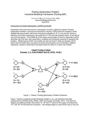
1. Pooling Optimization Problem
Industrial Modeling Framework (Pooling-IMF)
i n d u s t r IAL g o r i t h m s LLC. (IAL)
www.industrialgorithms.com
April 2014
Introduction to Pooling Optimization, UOPSS and QLQP
Presented in this short document is a description of what is called the (classic) “Pooling
Optimization Problem” and was first described in Haverly (1978) where he modeled a small
distillate blending problem with three component materials (A, B, C), one pool for mixing or
blending of only two components, two products (P1, P2) and one property (sulfur, S) as well as
only one time-period. The GAMS file of this exact same problem is found in Appendix A which
describes all of the sets, lists, parameters, variables and constraints required to represent this
problem. Related types of NLP sub-models can also be found in Kelly and Zyngier (2015)
where they formulate other sub-types of continuous-processes such as blenders, splitters,
separators, reactors, fractionators and black-boxes for adhoc or custom sub-models.
Figure 1. “Classic” Pooling Optimization Problem Flowsheet.
Figure 1 depicts a relatively simple flowsheet problem in our unit-operation-port-state
superstructure (UOPSS) (Kelly, 2004b, 2005, and Zyngier and Kelly, 2012). The diamond
shapes are called perimeter units where “A”, “B” and “C” stand for the supply of components,
“P1” and “P2” for the demand of products. The triangle shape is a pool which may or may not

2. have holdup or inventory where for this example the holdup lower and upper bounds are set to
zero (0) (see Appendix C for configuration details) . The circles indicate in-ports and out-ports
(with an “X” inside) which are known as the unambiguous flow interfaces in to and out of non-
port shapes where the entire flowsheet description or UOPS superstructure can be found in
Appendix B in the UPS file.
The label “S” denotes the sulfur property weight-percent values where for the component
materials they are fixed however for the products their upper bounds are shown with zero (0) as
an implied lower bounds. The “$” indicates the costs and prices used to maximize the objective
function of profit = product revenues - feed costs. The supplies of components are unlimited
whereas the demand flows of product have upper bounds of 100 and 200 weight-units
respectively.
Industrial Modeling Framework (IMF), IMPL and SIIMPLE
To implement the mathematical formulation of this and other systems, IAL offers a unique
approach and is incorporated into our Industrial Modeling Programming Language we call IMPL.
IMPL has its own modeling language called IML (short for Industrial Modeling Language) which
is a flat or text-file interface as well as a set of API's which can be called from any computer
programming language such as C, C++, Fortran, Java (SWIG), C#, VBA or Python (CTYPES)
called IPL (short for Industrial Programming Language) to both build the model and to view the
solution. Models can be a mix of linear, mixed-integer and nonlinear variables and constraints
and are solved using a combination of LP, QP, MILP and NLP solvers such as COINMP, GLPK,
LPSOLVE, SCIP, CPLEX, GUROBI, LINDO, XPRESS, CONOPT, IPOPT, KNITRO and
WORHP as well as our own implementation of SLP called SLPQPE (Successive Linear &
Quadratic Programming Engine) which is a very competitive alternative to the other nonlinear
solvers and embeds all available LP and QP solvers.
In addition and specific to DRR problems, we also have a special solver called SECQPE
standing for Sequential Equality-Constrained QP Engine which computes the least-squares
solution and a post-solver called SORVE standing for Supplemental Observability, Redundancy
and Variability Estimator to estimate the usual DRR statistics found in Kelly (1998 and 2004b)
and Kelly and Zyngier (2008a). SECQPE also includes a Levenberg-Marquardt regularization
method for nonlinear data regression problems and can be presolved using SLPQPE i.e.,
SLPQPE warm-starts SECQPE. SORVE is run after the SECQPE solver and also computes
the well-known "maximum-power" gross-error statistics (measurement and nodal/constraint
tests) to help locate outliers, defects and/or faults i.e., mal-functions in the measurement system
and mis-specifications in the logging system.
The underlying system architecture of IMPL is called SIIMPLE (we hope literally) which is short
for Server, Interfacer (IML), Interacter (IPL), Modeler, Presolver Libraries and Executable. The
Server, Presolver and Executable are primarily model or problem-independent whereas the
Interfacer, Interacter and Modeler are typically domain-specific i.e., model or problem-
dependent. Fortunately, for most industrial planning, scheduling, optimization, control and
monitoring problems found in the process industries, IMPL's standard Interfacer, Interacter and
Modeler are well-suited and comprehensive to model the most difficult of production and
process complexities allowing for the formulations of straightforward coefficient equations,
ubiquitous conservation laws, rigorous constitutive relations, empirical correlative expressions
and other necessary side constraints.

3. User, custom, adhoc or external constraints can be augmented or appended to IMPL when
necessary in several ways. For MILP or logistics problems we offer user-defined constraints
configurable from the IML file or the IPL code where the variables and constraints are
referenced using unit-operation-port-state names and the quantity-logic variable types. It is also
possible to import a foreign *.ILP file (row-based MPS file) which can be generated by any
algebraic modeling language or matrix generator. This file is read just prior to generating the
matrix and before exporting to the LP, QP or MILP solver. For NLP or quality problems we offer
user-defined formula configuration in the IML file and single-value and multi-value function
blocks writable in C, C++ or Fortran. The nonlinear formulas may include intrinsic functions
such as EXP, LN, LOG, SIN, COS, TAN, MIN, MAX, IF, NOT, EQ, NE, LE, LT, GE, GT and CIP,
LIP, SIP and KIP (constant, linear and monotonic spline interpolations) as well as user-written
extrinsic functions (XFCN). It is also possible to import another type of foreign file called the
*.INL file where both linear and nonlinear constraints can be added easily using new or existing
IMPL variables.
Industrial modeling frameworks or IMF's are intended to provide a jump-start to an industrial
project implementation i.e., a pre-project if you will, whereby pre-configured IML files and/or IPL
code are available specific to your problem at hand. The IML files and/or IPL code can be
easily enhanced, extended, customized, modified, etc. to meet the diverse needs of your project
and as it evolves over time and use. IMF's also provide graphical user interface prototypes for
drawing the flowsheet as in Figure 1 and typical Gantt charts and trend plots to view the solution
of quantity, logic and quality time-profiles. Current developments use Python 2.3 and 2.7
integrated with open-source Dia and Matplotlib modules respectively but other prototypes
embedded within Microsoft Excel/VBA for example can be created in a straightforward manner.
However, the primary purpose of the IMF's is to provide a timely, cost-effective, manageable
and maintainable deployment of IMPL to formulate and optimize complex industrial
manufacturing systems in either off-line or on-line environments. Using IMPL alone would be
somewhat similar (but not as bad) to learning the syntax and semantics of an AML as well as
having to code all of the necessary mathematical representations of the problem including the
details of digitizing your data into time-points and periods, demarcating past, present and future
time-horizons, defining sets, index-sets, compound-sets to traverse the network or topology,
calculating independent and dependent parameters to be used as coefficients and bounds and
finally creating all of the necessary variables and constraints to model the complex details of
logistics and quality industrial optimization problems. Instead, IMF's and IMPL provide, in our
opinion, a more elegant and structured approach to industrial modeling and solving so that you
can capture the benefits of advanced decision-making faster, better and cheaper.
Pooling Optimization Problem Synopsis
At this point we explore further the solution of this small but representative mono-pool, mono-
property and mono-period pooling problem. Since there are at least bilinear terms with plus and
minus coefficients (see poolqualbal() and blendqualbal()in GAMS file) this problem is
non-convex and may exhibit one or more local optima. In fact, this problem is extremely well-
studied in the global optimization literature where there are three (3) known local optima of $0,
$100 and $400.
To show the optimization results clearly, we have coded this problem into Microsoft Excel VBA
using IMPL’s Industrial Programming Language (IPL) API’s where we have superimposed the
weight flow solutions in green with the flowsheet (see Figures 2 and 3). * Please note that the
IMPL *.xlsm file may be provided at the readers request.

4. Figure 2. Pooling Optimization Problem in Microsoft Excel VBA ($100).
Figure 3. Pooling Optimization Problem in Microsoft Excel VBA ($400).
To solve this problem we use IMPL’s SLPQPE solver with COINMP as the LP sub-solver
although IPOPT, etc. may also be used. In order to perturb the model-data to arrive at two of

5. the local optimum ($100 and $400), we randomize the initial-values or starting-points using the
technique found in Chinneck (2008) which is a standard feature in IMPL (see the cell (I2)
labeled “Seed”). These same solutions are found in the global optimization literature.
Contrasting GAMS with IMPL, to use GAMS you need to need to both “code the model” and
“configure the data” whereas in IMPL you only need to “configure the data” given that all of the
sets, lists, parameters, variables and constraints are already available in IMPL for these types of
industrial optimization problems (compare Appendix A with Appendix C). With IMPL, all of the
modeling data structures are conveniently indexed, addressed or pointed to using our unit-
operation-port-state superstructure (UOPSS) and our quantity-logic-quality phenomena (QLQP)
so the developer-user does not need to be burdened with creating or generating their own data
structures for each problem type as is usually the case with GAMS and the other algebraic
modeling languages such as AIMMS, AMPL, MPL, LINGO, MOSEL, ZIMPL, etc.
In addition, it also takes great skill to determine for each type of problem how to code or create
all of the mathematical structures (i.e., variables and constraints) required to model a problem
with sufficient accuracy of industrial significance that can generate significant benefits or
savings for your company. Again with IMPL, this burden is also drastically reduced as well as
other aspects such as digitizing/discretizing the data over many time-periods, handling all forms
of infeasibilities, generating useful initial-values for nonlinear problems, fitting coefficients to past
industrial data for more accurate models (parameter estimation and data reconciliation),
integrating planning (NLP) and scheduling (MILP) problems seamlessly, customizing relaxation,
decomposition and other primal heuristics to solve large-scale problems quickly and effectively,
etc.
References
Haverly, C.A., “Studies of the behavior of recursion for the pooling problem”, ACM SIGMAP
Bulletin, 25, 19-28, (1978).
Kelly, J.D., "Formulating production planning models", Chemical Engineering Progress,
January, 43, (2004a).
Kelly, J.D., "Production modeling for multimodal operations", Chemical Engineering Progress,
February, 44, (2004b).
Kelly, J.D., "The unit-operation-stock superstructure (UOSS) and the quantity-logic-quality
paradigm (QLQP) for production scheduling in the process industries", In: MISTA 2005
Conference Proceedings, 327, (2005).
Chinneck, J.W., “Feasibility and infeasibility in optimization: algorithms and computational
methods, Springer Science, New York, (2008).
Zyngier, D., Kelly, J.D., "UOPSS: a new paradigm for modeling production planning and
scheduling systems", ESCAPE 22, June, (2012).
Kelly, J.D., Zyngier, D., "Unit operation nonlinear modeling for planning and scheduling
applications", K.C. Furman et.al. (eds.), Optimization and Analytics in the Oil & Gas Industries,
Springer Science, (2015).
Appendix A - GAMS File (http://www.gams.com/modlib/libhtml/haverly.htm)

6. $title Haverly's pooling problem example (HAVERLY,SEQ=214)
$ontext
Haverly's pooling problem example. This is a non-convex problem.
Setting initial levels for the nonlinear variables is a good
approach to find the global optimum.
Haverly, C A, Studies of the Behavior of Recursion for the Pooling
Problem. ACM SIGMAP Bull 25 (1978), 29-32.
Adhya, N, Tawaralani, M, and Sahinidis, N, A Lagrangian Approach to
the Pooling Problem. Independent Engineering Chemical Research 38
(1999), 1956-1972.
----- crudeA ------/--- pool --|
/ |--- finalX
----- crudeB ----/ |
|--- finalY
----- crudeC ------------------|
$offtext
sets s supplies (crudes) / crudeA, crudeB, crudeC /
f final products / finalX, finalY /
i intermediate sources for final products / Pool, CrudeC /
poolin(s) crudes going into pool tank / crudeA, crudeB /
table data_S(s,*) supply data summary
price sulfur
crudeA 6 3
crudeB 16 1
crudeC 10 2
table data_f(f,*) final product data
price sulfur demand
finalX 9 2.5 100
finalY 15 1.5 200
parameters sulfur_content(s) supply quality in (percent)
req_sulfur(f) required max sulfur content (percentage)
demand(f) final product demand;
sulfur_content(s) = data_S(s,'sulfur');
req_sulfur(f) = data_F(f,'sulfur');
demand(f) = data_F(f,'demand');
equations
costdef cost equation
incomedef income equation
blend(f) blending of final products
poolbal pool tank balance
crudeCbal balance for crudeC
poolqualbal pool quality balance
blendqualbal quality balance for blending
profitdef profit equation
positive variables
crude(s) amount of crudes being used
stream(i,f) streams
q pool quality
variables
profit total profit
cost total costs
income total income
final(f) amount of final products sold;
profitdef.. profit =e= income - cost;
costdef.. cost =e= sum(s, data_S(s,'price')*crude(s));
incomedef.. income =e= sum(f, data_F(f,'price')*final(f));
blend(f).. final(f) =e= sum(i, stream(i,f));
poolbal.. sum(poolin, crude(poolin)) =e= sum(f, stream('pool',f));
crudeCbal.. crude('crudeC') =e= sum(f, stream('crudeC',f));
poolqualbal.. q*sum(f, stream('pool', f)) =e=
sum(poolin, sulfur_content(poolin)*crude(poolin));
blendqualbal(f)..
q*stream('pool',f) + sulfur_content('CrudeC')*stream('CrudeC',f)
=l= req_sulfur(f)*sum(i,stream(i,f));
final.up(f) = demand(f);
model m /all/;

7. * Because of the product terms, some local solver may get
* trapped at 0*0, we therefore set an initial value for q.
q.l=1;
solve m maximizing profit using nlp;
Appendix B - Pooling-IMF.UPS (UOPSS) File
i M P l (c)
Copyright and Property of i n d u s t r I A L g o r i t h m s LLC.
checksum,39
!!!!!!!!!!!!!!!!!!!!!!!!!!!!!!!!!!!!!!!!!!!!!!!!!!!!!!!!!!!!!!
! Unit-Operation-Port-State-Superstructure (UOPSS) *.UPS File.
! (This file is automatically generated from the Python program IALConstructer.py)
!!!!!!!!!!!!!!!!!!!!!!!!!!!!!!!!!!!!!!!!!!!!!!!!!!!!!!!!!!!!!!
&sUnit,&sOperation,@sType,@sSubtype,@sUse
A,,perimeter,,
B,,perimeter,,
C,,perimeter,,
P1,,perimeter,,
P2,,perimeter,,
Pool,,pool,,
&sUnit,&sOperation,@sType,@sSubtype,@sUse
! Number of UO shapes = 6
&sAlias,&sUnit,&sOperation
ALLPARTS,A,
ALLPARTS,B,
ALLPARTS,C,
ALLPARTS,P1,
ALLPARTS,P2,
ALLPARTS,Pool,
&sAlias,&sUnit,&sOperation
&sUnit,&sOperation,&sPort,&sState,@sType,@sSubtype
A,,o,,out,
B,,o,,out,
C,,o,,out,
P1,,i,,in,
P2,,i,,in,
Pool,,i,,in,
Pool,,o,,out,
&sUnit,&sOperation,&sPort,&sState,@sType,@sSubtype
! Number of UOPS shapes = 7
&sAlias,&sUnit,&sOperation,&sPort,&sState
ALLINPORTS,P1,,i,
ALLINPORTS,P2,,i,
ALLINPORTS,Pool,,i,
ALLOUTPORTS,A,,o,
ALLOUTPORTS,B,,o,
ALLOUTPORTS,C,,o,
ALLOUTPORTS,Pool,,o,
&sAlias,&sUnit,&sOperation,&sPort,&sState
&sUnit,&sOperation,&sPort,&sState,&sUnit,&sOperation,&sPort,&sState
A,,o,,Pool,,i,
B,,o,,Pool,,i,
C,,o,,P1,,i,
C,,o,,P2,,i,
Pool,,o,,P1,,i,
Pool,,o,,P2,,i,
&sUnit,&sOperation,&sPort,&sState,&sUnit,&sOperation,&sPort,&sState
&sAlias,&sUnit,&sOperation,&sPort,&sState,&sUnit,&sOperation,&sPort,&sState
ALLPATHS,C,,o,,P1,,i,
ALLPATHS,Pool,,o,,P1,,i,
ALLPATHS,C,,o,,P2,,i,
ALLPATHS,Pool,,o,,P2,,i,
ALLPATHS,A,,o,,Pool,,i,
ALLPATHS,B,,o,,Pool,,i,
&sAlias,&sUnit,&sOperation,&sPort,&sState,&sUnit,&sOperation,&sPort,&sState
Appendix C - Pooling-IMF.IML File
i M P l (c)
Copyright and Property of i n d u s t r I A L g o r i t h m s LLC.
!!!!!!!!!!!!!!!!!!!!!!!!!!!!!!!!!!!!!!!!!!!!!!!!!!!!!!!!!!!!!!!!!!!!!!!!!!!!!!!!
! Calculation Data (Parameters)
!!!!!!!!!!!!!!!!!!!!!!!!!!!!!!!!!!!!!!!!!!!!!!!!!!!!!!!!!!!!!!!!!!!!!!!!!!!!!!!!

8. &sCalc,@sValue
START,-1.0
BEGIN,0.0
END,1.0
PERIOD,1.0
&sCalc,@sValue
!!!!!!!!!!!!!!!!!!!!!!!!!!!!!!!!!!!!!!!!!!!!!!!!!!!!!!!!!!!!!!!!!!!!!!!!!!!!!!!!
! Chronological Data (Periods)
!!!!!!!!!!!!!!!!!!!!!!!!!!!!!!!!!!!!!!!!!!!!!!!!!!!!!!!!!!!!!!!!!!!!!!!!!!!!!!!!
@rPastTHD,@rFutureTHD,@rTPD
START,END,PERIOD
@rPastTHD,@rFutureTHD,@rTPD
!!!!!!!!!!!!!!!!!!!!!!!!!!!!!!!!!!!!!!!!!!!!!!!!!!!!!!!!!!!!!!!!!!!!!!!!!!!!!!!!
! Construction Data (Pointers)
!!!!!!!!!!!!!!!!!!!!!!!!!!!!!!!!!!!!!!!!!!!!!!!!!!!!!!!!!!!!!!!!!!!!!!!!!!!!!!!!
Include-@sFile_Name
Pooling-IMF.ups
Include-@sFile_Name
!!!!!!!!!!!!!!!!!!!!!!!!!!!!!!!!!!!!!!!!!!!!!!!!!!!!!!!!!!!!!!!!!!!!!!!!!!!!!!!!
! Capacity Data (Prototypes)
!!!!!!!!!!!!!!!!!!!!!!!!!!!!!!!!!!!!!!!!!!!!!!!!!!!!!!!!!!!!!!!!!!!!!!!!!!!!!!!!
&sUnit,&sOperation,@rRate_Lower,@rRate_Upper
ALLPARTS,0.0,1000.0
&sUnit,&sOperation,@rRate_Lower,@rRate_Upper
&sUnit,&sOperation,@rHoldup_Lower,@rHoldup_Upper
Pool,,0.0,0.0
&sUnit,&sOperation,@rHoldup_Lower,@rHoldup_Upper
&sUnit,&sOperation,&sPort,&sState,@rTeeRate_Lower,@rTeeRate_Upper
ALLINPORTS,0.0,1000.0
ALLOUTPORTS,0.0,1000.0
&sUnit,&sOperation,&sPort,&sState,@rTeeRate_Lower,@rTeeRate_Upper
&sUnit,&sOperation,&sPort,&sState,@rTotalRate_Lower,@rTotalRate_Upper
ALLINPORTS,0.0,1000.0
ALLOUTPORTS,0.0,1000.0
P1,,i,,0.0,100.0
P2,,i,,0.0,200.0
&sUnit,&sOperation,&sPort,&sState,@rTotalRate_Lower,@rTotalRate_Upper
!!!!!!!!!!!!!!!!!!!!!!!!!!!!!!!!!!!!!!!!!!!!!!!!!!!!!!!!!!!!!!!!!!!!!!!!!!!!!!!!
! Constituent Data (Properties)
!!!!!!!!!!!!!!!!!!!!!!!!!!!!!!!!!!!!!!!!!!!!!!!!!!!!!!!!!!!!!!!!!!!!!!!!!!!!!!!!
&sProperty
S
&sProperty
&sUnit,&sOperation,&sPort,&sState,&sProperty,@rProperty_Lower,@rProperty_Upper,@rProperty_Target
ALLINPORTS,S,0.0,3.0
ALLOUTPORTS,S,0.0,3.0
A,,o,,S,3.0,3.0
B,,o,,S,1.0,1.0
C,,o,,S,2.0,2.0
P1,,i,,S,0.0,2.5
P2,,i,,S,0.0,1.5
&sUnit,&sOperation,&sPort,&sState,&sProperty,@rProperty_Lower,@rProperty_Upper,@rProperty_Target
!!!!!!!!!!!!!!!!!!!!!!!!!!!!!!!!!!!!!!!!!!!!!!!!!!!!!!!!!!!!!!!!!!!!!!!!!!!!!!!!
! Cost Data (Pricing)
!!!!!!!!!!!!!!!!!!!!!!!!!!!!!!!!!!!!!!!!!!!!!!!!!!!!!!!!!!!!!!!!!!!!!!!!!!!!!!!!
&sUnit,&sOperation,&sPort,&sState,@rFlowPro_Weight,@rFlowPer1_Weight,@rFlowPer2_Weight,@rFlowPen_Weight
A,,o,,-6.0
B,,o,,-16.0
C,,o,,-10.0
P1,,i,,9.0
P2,,i,,15.0
&sUnit,&sOperation,&sPort,&sState,@rFlowPro_Weight,@rFlowPer1_Weight,@rFlowPer2_Weight,@rFlowPen_Weight
!!!!!!!!!!!!!!!!!!!!!!!!!!!!!!!!!!!!!!!!!!!!!!!!!!!!!!!!!!!!!!!!!!!!!!!!!!!!!!!!
! Command Data (Future Provisos)
!!!!!!!!!!!!!!!!!!!!!!!!!!!!!!!!!!!!!!!!!!!!!!!!!!!!!!!!!!!!!!!!!!!!!!!!!!!!!!!!
&sUnit,&sOperation,@rSetup_Lower,@rSetup_Upper,@rBegin_Time,@rEnd_Time
ALLPARTS,1,1,BEGIN,END
&sUnit,&sOperation,@rSetup_Lower,@rSetup_Upper,@rBegin_Time,@rEnd_Time
&sUnit,&sOperation,&sPort,&sState,&sUnit,&sOperation,&sPort,&sState,@rSetup_Lower,@rSetup_Upper,@rBegin_Time,@rEnd_Time
ALLPATHS,1,1,BEGIN,END
&sUnit,&sOperation,&sPort,&sState,&sUnit,&sOperation,&sPort,&sState,@rSetup_Lower,@rSetup_Upper,@rBegin_Time,@rEnd_Time